D-optimal design for multivariate polynomial regression via the Christoffel function and semidefinite relaxations
Yohann De Castro (LM-Orsay), F Gamboa (IMT), D Henrion (LAAS-MAC,, CTU), R Hess (LAAS-MAC), J.-B Lasserre (LAAS-MAC, IMT)

TL;DR
This paper introduces a novel method for designing D-optimal experiments in multivariate polynomial regression using semidefinite programming and Christoffel functions, enabling efficient numerical solutions and geometric interpretation.
Contribution
It develops a new approach combining moment-sum-of-squares hierarchy and Christoffel polynomial for optimal experimental design in polynomial regression.
Findings
Effective numerical approximation of D-optimal designs.
Utilization of semidefinite programming duality for geometric insights.
Applicable to compact semi-algebraic design spaces.
Abstract
We present a new approach to the design of D-optimal experiments with multivariate polynomial regressions on compact semi-algebraic design spaces. We apply the moment-sum-of-squares hierarchy of semidefinite programming problems to solve numerically and approximately the optimal design problem. The geometry of the design is recovered with semidefinite programming duality theory and the Christoffel polynomial.
Click any figure to enlarge with its caption.
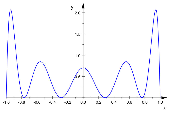 Figure 1
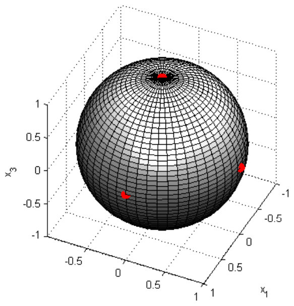 Figure 2
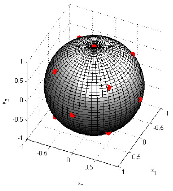 Figure 3
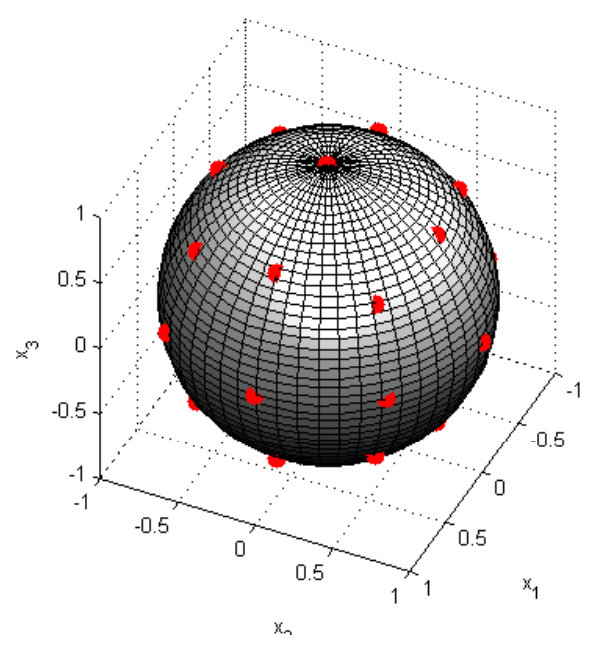 Figure 4
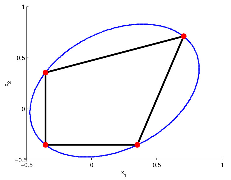 Figure 5
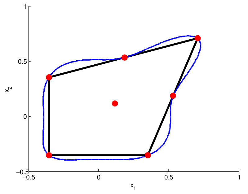 Figure 6
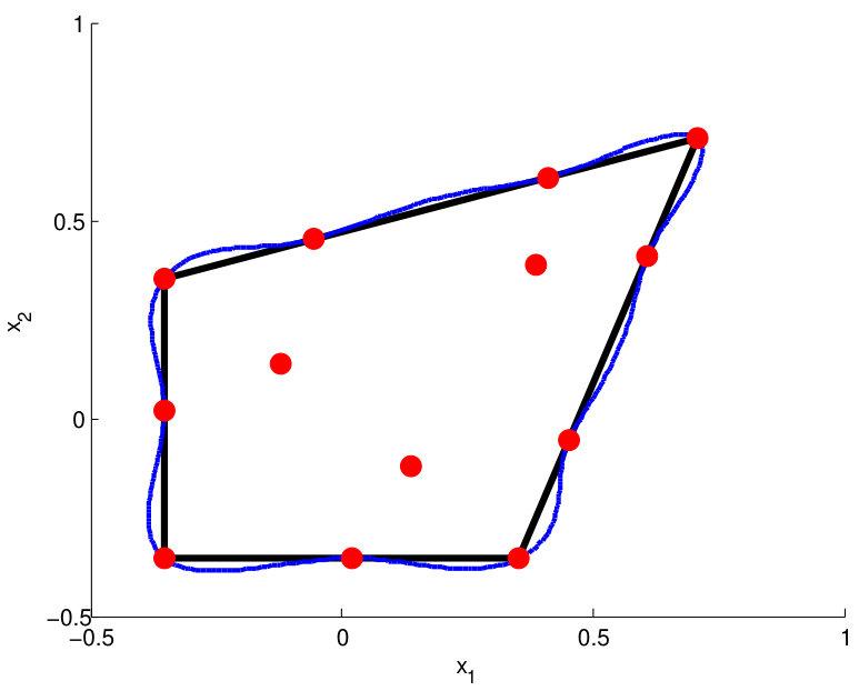 Figure 7
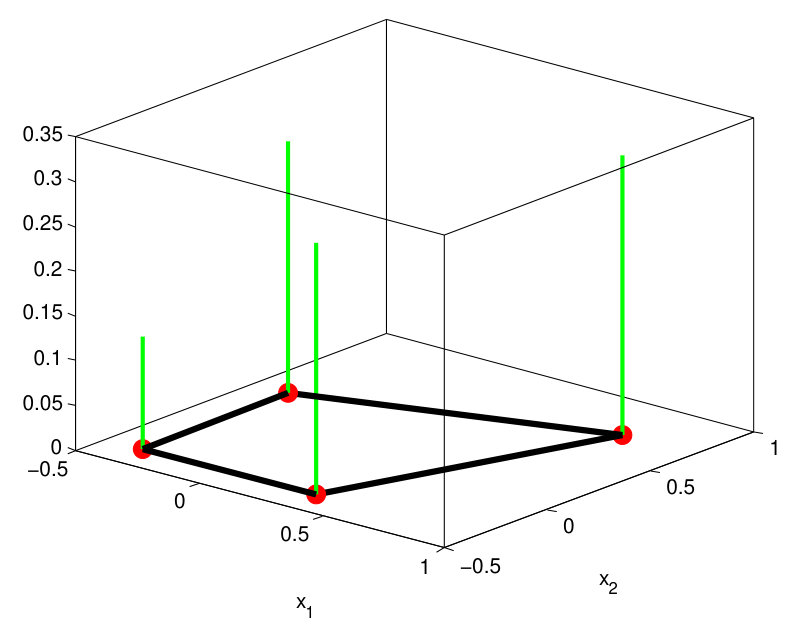 Figure 8
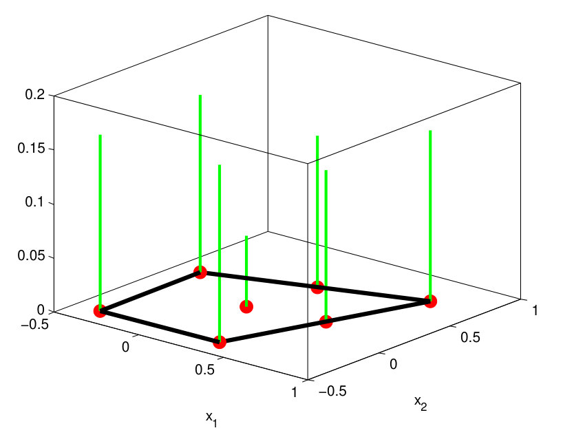 Figure 9
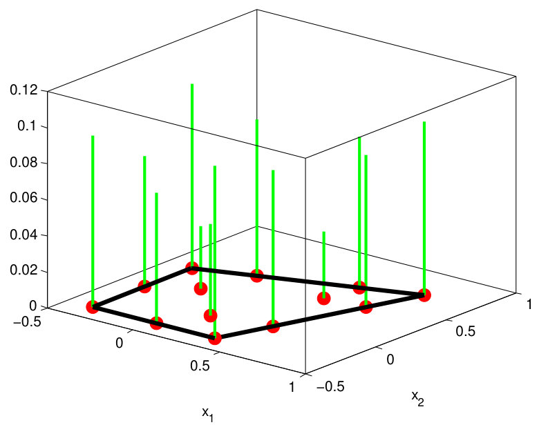 Figure 10
Peer Reviews
No public reviews on file for this paper yet. If you reviewed it on a platform where reviews are public (OpenReview, ICLR, NeurIPS, ICML), you can paste yours below so the community can read it here.
Videos
No videos yet. Explain this paper in a talk, walkthrough, or lecture? Add one.
Taxonomy
TopicsOptimal Experimental Design Methods · Probabilistic and Robust Engineering Design · Advanced Multi-Objective Optimization Algorithms
D-optimal design for multivariate polynomial regression via the Christoffel function and semidefinite relaxations
Y. De Castro and F. Gamboa and D. Henrion and R. Hess and J.-B. Lasserre
YDC is with the Laboratoire de Mathématiques d’Orsay, Univ. Paris-Sud, CNRS, Université Paris-Saclay, 91405 Orsay, France.
[email protected] www.math.u-psud.fr/$\sim$decastro FG is with the Institut de Mathématiques de Toulouse (CNRS UMR 5219), Université Paul Sabatier, 118 route de Narbonne, 31062 Toulouse, France.
[email protected] www.math.univ-toulouse.fr/$\sim$gamboa DH is with LAAS-CNRS, Université de Toulouse, LAAS, 7 avenue du colonel Roche, F-31400 Toulouse, France and with the Faculty of Electrical Engineering, Czech Technical University in Prague, Technická 2, CZ-16626 Prague, Czech Republic
[email protected] homepages.laas.fr/henrion RH is with LAAS-CNRS, Université de Toulouse, LAAS, 7 avenue du colonel Roche, F-31400 Toulouse, France.
JBL is with LAAS-CNRS, Université de Toulouse, LAAS, 7 avenue du colonel Roche, F-31400 Toulouse, France.
[email protected] homepages.laas.fr/lasserre
(Date: Draft of March 2, 2024)
Abstract.
We present a new approach to the design of D-optimal experiments with multivariate polynomial regressions on compact semi-algebraic design spaces. We apply the moment-sum-of-squares hierarchy of semidefinite programming problems to solve numerically and approximately the optimal design problem. The geometry of the design is recovered with semidefinite programming duality theory and the Christoffel polynomial.
Key words and phrases:
Experimental design; semidefinite programming
1. Introduction
1.1. Convex design theory
The optimum experimental designs are computational and theoretical objects that minimize the variance of the best linear unbiased estimators in regression problems. In this frame, the experimenter models the responses of a random experiment whose inputs are represented by a vector with respect to known regression functions , namely
[TABLE]
where are unknown parameters that the experimenter wants to estimate, is some noise and the inputs are chosen by the experimenter in a design space . Assume that the inputs , for , are chosen within a set of distinct points with , and let denote the number of times the particular point occurs among . This would be summarized by
[TABLE]
whose first row gives the points in the design space where the inputs parameters have to be taken and the second row indicates the experimenter which proportion of experiments (frequencies) have to be done at these points. The goal of the design of experiment theory is then to assess which input parameters and frequencies the experimenter has to consider. For a given the standard analysis of the Gaussian linear model shows that the minimal covariance matrix (with respect to Loewner ordering) of unbiased estimators can be expressed in terms of the Moore-Penrose pseudoinverse of the information matrix which is defined by
[TABLE]
where is the column vector of regression functions. One major aspect of design of experiment theory seeks to maximize the information matrix over the set of all possible . Notice the Loewner ordering is partial and, in general, there is no greatest element among all possible information matrices . The standard approach is then to consider some statistical criteria, namely Kiefer’s -criteria [K74], in order to describe and construct the “optimal designs” with respect to those criteria. Observe that the information matrix belongs to , the space of symmetric nonnegative definite matrices of size , and for all define the function
[TABLE]
where for positive definite matrices it holds
[TABLE]
and for nonnegative definite matrices it holds
[TABLE]
Those criteria are meant to be real valued, positively homogeneous, non constant, upper semi-continuous, isotonic (with respect to the Loewner ordering) and concave functions. Throughout this paper, we restrict ourselves to the -optimality criteria which corresponds to the choice . Other criteria will be studied elsewhere.
In particular, in this paper we search for solutions to the following optimization problem
[TABLE]
where the maximum is taken over all of the form (1.1). Note that the logarithm of the determinant is used instead of because of its standard use in semidefinite programming (SDP) as a barrier function for the cone of positive definite matrices.
1.2. State of the art
Optimal design is at the heart of statistical planning for inference in the linear model, see for example [BHH78]. While the case of discrete input factors is generally tackled by algebraic and combinatoric arguments (e.g., [B08]), the one of continuous input factors often leads to an optimization problem. In general, the continuous factors are generated by a vector of linearly independent regular functions on the design space . One way to handle the problem is to focus only on ignoring the function and to try to draw the design points filling the best the set . This is generally done by optimizing a cost function on that traduces the way the design points are positioned between each other and/or how they fill the space. Generic examples are the so-called maxmin or minmax criteria (see for example [PW88] or [WPN97]) and the minimum discrepancy designs (see for example [LQX05]). Another point of view—which is the one developed here—relies on the maximization of the information matrix. Of course, as explained before, the Loewner order is partial and so the optimization can not stand on this matrix but on one of its feature. A pioneer paper adopting this point of view is the one of Elfving [E52]. In the early 60’s, in a series of papers, Kiefer and Wolwofitz shade new lights on this kind of methods for experimental design by introducing the equivalence principle and proposing in some cases algorithms to solve the optimization problem, see [K74] and references therein. Following the early works of Karlin and Studden ([KS66b], [KS66a]), the case of polynomial regression on a compact interval on has been widely studied. In this frame, the theory is almost complete an many thing can be said about the optimal solutions for the design problem (see [DS93]). Roughly speaking, the optimal design points are related to the zeros of orthogonal polynomials built on an equilibrum measure. We refer to the excelent book of Dette and Studden [DS97] and reference therein for a complete overview on the subject. In the one dimensional frame, other systems of functions (trigonometric functions or some -system, see [KN77] for a definition) are studied in a same way in [DS97], [LS85] and [IS01]. In the multidimensional case, even for polynomial systems, very few case of explicit solutions are known. Using tensoring arguments the case of a rectangle is treated in [DS97]. Particular models of degree two are studied in [DG14] and [PW94]. Away from these particular cases, the construction of the optimal design relies on numerical optimization procedures. The case of the determinant (-optimality) is studied for example in [W70] and [VBW98]. An other criterion based on matrix conditioning is developed in [MYZ14]. General optimization algorithm are discussed in [F10] and [ADT07]. In the frame of fixed given support points efficient SDP based algorithms are proposed and studied in [S11] and [SH15]. Let us mention, the paper [VBW98] which is one of the original motivation to develop SDP solvers, especially for Max Det Problems (corresponding to -optimal design) and the so-called problem of analytical centering.
1.3. Contribution
For the first time, this paper introduces a general method to compute the approximate -optimal designs on a large variety of design spaces that we referred to as semi-algebraic sets, see [L10] for a definition. This family can be understood as any sets given by intersections and complements of the level sets of multivariate polynomials. The theoretical guarantees are given by Theorems 4.3 and 4.4. We apply the moment-sum-of-squares hierarchy (a.k.a. the Lasserre hierarchy) of SDP problems to solve numerically and approximately the optimal design problem They show the convergence of our method towards the optimal information matrix as the order of the hierarchy increases. Furthermore, we show that our method recovers the optimal design when finite convergence of this hierarchy occurs. To recover the geometry of the design we use SDP duality theory and the Christoffel polynomial. We have run several numerical experiments for which finite convergence holds leading to a surprisingly fast and reliable method to compute optimal designs. As illustrated by our examples, using Christoffel polynomials of degrees higher than two allows to reconstruct designs with points in the interior of the domain, contrasting with the classical use of ellipsoids for linear regressions.
1.4. Outline of the paper
In Section 2, after introducing necessary notation, we shortly explain some basics on moments and moment matrices, and present the approximation of the moment cone via the Lasserre hierarchy. Section 3 is dedicated to further describing optimum designs and their approximations. At the end of the section we propose a two step procedure to solve the approximate design problem. Solving the first step is subject to Section 4. There, we find a sequence of moments associated with the optimal design measure. Recovering this measure (step two of the procedure) is discussed in Section 5. We finish the paper with some illustrating examples and a conclusion.
2. Polynomial optimal design and moments
This section collects preliminary material on semialgebraic sets, moments and moment matrices, using the notations of [L10]. This material will be used to restrict our attention to polynomial optimal design problems with polynomial regression functions and semi-algebraic design spaces.
2.1. Polynomial optimal design
Denote by the vector space of real polynomials in the variables , and for , define where denotes the total degree of .
In this paper we assume that the regression functions are multivariate polynomials, i.e. . Moreover, we consider that the design space is a given closed basic semi-algebraic set
[TABLE]
for given polynomials , , whose degrees are denoted by , . Assume that is compact with an algebraic certificate of compactness. For example, one of the polynomial inequalities should be of the form for a sufficiently large constant .
Notice that those assumptions cover a large class of problems in optimal design theory, see for instance [DS97, Chapter 5]. In particular, observe that the design space defined by (2.1) is not necessarily convex and note that the polynomial regressors can handle incomplete -way th degree polynomial regression.
The monomials , with , form a basis of the vector space . We use the multi-index notation to denote these monomials. In the same way, for a given the vector space has dimension with basis , where . We write
[TABLE]
for the column vector of the monomials ordered according to their degree, and where monomials of the same degree are ordered with respect to the lexicographic ordering.
The cone of nonnegative Borel measures supported on is understood as the dual to the cone of nonnegative elements of the space of continuous functions on .
2.2. Moments, the moment cone and the moment matrix
Given and , we call
[TABLE]
the moment of order of . Accordingly, we call the sequence the moment sequence of . Conversely, we say that a sequence has a representing measure, if there exists a measure such that is its moment sequence.
We denote by the convex cone of all truncated sequences which have a representing measure supported on . We call it the moment cone of . It can be expressed as
[TABLE]
We also denote by the convex cone of polynomials of degree at most that are nonnegative on . When is compact then and (see e.g. [L15][Lemma 2.5]).
When the design space is given by the univariate interval , i.e., , then this cone is representable using positive semidefinite Hankel matrices, which implies that convex optimization on this cone can be carried out with efficient interior point algorithms for semidefinite programming, see e.g. [VBW98]. Unfortunately, in the general case, there is no efficient representation of this cone. It has actually been shown in [S16] that the moment cone is not semidefinite representable, i.e. it cannot be expressed as the projection of a linear section of the cone of positive semidefinite matrices. However, we can use semidefinite approximations of this cone as discussed in Section 2.3.
Given a sequence we define the linear functional which maps a polynomial to
[TABLE]
A sequence has a representing measure supported on if and only if for all polynomials nonnegative on [L10, Theorem 3.1].
The moment matrix of a truncated sequence is the -matrix with rows and columns respectively indexed by and whose entries are given by
[TABLE]
It is symmetric and linear in , and if has a representing measure, then is positive semidefinite, denoted by .
Similarly, we define the localizing matrix of a polynomial of degree and a sequence as the -matrix with rows and columns respectively indexed by and whose entries are given by
[TABLE]
If has a representing measure , then for whenever the support of is contained in the set .
Since is basic semialgebraic with a certificate of compactness, by Putinar’s theorem [L10, Theorem 3.8], we also know the converse statement in the infinite case, namely has a representing measure if and only if for all the matrices and , are positive semidefinite.
2.3. Approximations of the moment cone
Letting , , for half the degree of the , by Putinar’s theorem, we can approximate the moment cone by the following semidefinite representable cones for
[TABLE]
By semidefinite representable we mean that the cones are projections of linear sections of semidefinite cones. Since is contained in every , they are outer approximations of the moment cone. Moreover, they form a nested sequence, so we can build the hierarchy
[TABLE]
This hierarchy actually converges, meaning , where denotes the topological closure of the set .
3. Approximate Optimal Design
3.1. Problem reformulation in the multivariate polynomial case
For all and , let with appropriate . Define for with moment sequence the information matrix
[TABLE]
where we have set A_{\gamma}:=\Big{(}\sum_{\alpha+\beta=\gamma}a_{i,\alpha}a_{j,\beta}\Big{)}_{1\leq i,j\leq p} for .
Further, let where denotes the Dirac measure at the point and observe that as in (1.2).
The optimization problem
[TABLE]
where the maximization is with respect to and , , subject to the constraint that the information matrix is positive semidefinite, is by construction equivalent to the original design problem (1.3). In this form, problem (3.1) is difficult because of the integrality constraints on the and the nonlinear relation between , and . We will address these difficulties in the sequel by first relaxing the integrality constraints.
3.2. Relaxing the integrality constraints
In problem 3.1, the set of admissible frequencies is discrete, which makes it a potentially difficult combinatorial optimization problem. A popular solution is then to consider “approximate” designs defined by
[TABLE]
where the frequencies belong to the unit simplex . Accordingly, any solution to (1.3) where the maximum is taken over all matrices of type (3.2) is called “approximate optimal design”, yielding the following relaxation of problem 3.1
[TABLE]
where the maximization is with respect to and , , subject to the constraint that the information matrix is positive semidefinite. In this problem, the nonlinear relation between , and is still an issue.
3.3. Moment formulation
Let us introduce a two-step-procedure to solve the approximate optimal design problem (3.3). For this we will first again reformulate our problem.
Observe that by Carathéodory’s theorem, the truncated moment cone defined in (2.2) is exactly
[TABLE]
so that problem (3.2) is equivalent to
[TABLE]
where the maximization is now with respect to the sequence . Moment problem (3.4) is finite-dimensional and convex, yet the constraint is difficult to handle. We will show that by approximating the truncated moment cone by a nested sequence of semidefinite representable cones as indicated in (2.3), we obtain a hierarchy of finite dimensional semidefinite programming problems converging to the optimal solution of (3.4). Since semidefinite programming problems can be solved efficiently, we can compute a numerical solution to problem (3.2).
This describes step one of our procedure. The result of it is a sequence of moments. Consequently, in a second step, we need to find a representing atomic measure of in order to identify the approximate optimum design .
4. The ideal problem on moments and its approximation
For notational simplicity, let us use the standard monomial basis of for the regression functions, meaning with . Note that this is not a restriction, since one can get the results for other choices of by simply performing a change of basis. Different polynomial bases can be considered and one may consult the standard framework described by [DS97, Chapter 5.8]. For the sake of conciseness, we do not expose the notion of incomplete -way -th degree polynomial regression here but the reader may remark that the strategy developed in this paper can handle such a framework.
4.1. Christoffel polynomials
It turns out that the (unique) optimal solution of (3.4) can be characterized in terms of the Christoffel polynomial of degree associated with an optimal measure whose moments up to order coincide with .
Definition 4.1**.**
Let be such that . Then there exists a family of orthonormal polynomials satisfying
[TABLE]
where monomials are ordered with the lexicographical ordering on . We call the polynomial
[TABLE]
the Christoffel polynomial (of degree ) associated with .
The Christoffel polynomial111In fact what is referred to in the literature is its reciprocal called the Chistoffel function. can be expressed in different ways. For instance via the inverse of the moment matrix by
[TABLE]
or via its extremal property
[TABLE]
when has a representing measure . (When does not have a representing measure just replace with )). For more details the interested reader is referred to [LP16] and the references therein.
4.2. The ideal problem on moments
The ideal formulation (3.4) of our approximate optimal design problem reads
[TABLE]
For this we have the following result
Theorem 4.2**.**
Let be compact with nonempty interior. Problem (4.1) is a convex optimization problem with a unique optimal solution . It is the vector of moments (up to order ) of a measure supported on at least and at most points in the set where and is the Christoffel polynomial
[TABLE]
Proof.
First, let us prove that (4.1) has an optimal solution. The feasible set is nonempty (take as feasible point the vector associated with the Lebesgue measure on , scaled to be a probability measure) with finite associated objective value, because . Hence, and in addition Slater’s condition holds because (that is, is a strictly feasible solution to (4.1)).
Next, as is compact there exists such that for every probability measure on and every . Hence, which by [LN07] implies that for every , which in turn implies that the feasible set of (4.1) is compact. As the objective function is continuous and , problem (4.1) has an optimal solution .
Furthermore, an optimal solution is unique because the objective function is strictly convex and the feasible set is convex. In addition, since , and so is non singular.
Next, writing , , for the real matrices satisfying and for two matrices and , the necessary Karush-Kuhn-Tucker optimality conditions222For the optimization problem where is differentiable, and is a nonempty closed convex cone, the KKT-optimality conditions at a feasible point state that there exists and such that and . Slater’s condition holds if there exists a feasible solution , in which case the KKT-optimality conditions are necessary and sufficient if is convex. (in short KKT-optimality conditions) state that an optimal solution should satisfy
[TABLE]
(where and is the dual variable associated with the constraint ), with the complementarity condition . That is:
[TABLE]
Multiplying (4.3) term-wise by , summing up and invoking the complementarity condition, yields
[TABLE]
Similarly, multiplying (4.3) term-wise by and summing up yields
[TABLE]
where the , , are the orthonormal polynomials (up to degree ) w.r.t. , where is a representing measure of (recall that ). Therefore where is the Christoffel polynomial of degree associated with . Next, the complementarity condition reads
[TABLE]
which implies that the support of is included in the algebraic set . Finally, that is an atomic measure supported on at most points follows from Tchakaloff’s theorem [L10, Theorem B.12] which states that for every finite Borel probability measure on and every , there exists an atomic measure supported on points such that all moments of and agree up to order . So let . Then . If , then in contradiction to being non-singular. Therefore, . ∎
So we obtain a nice characterization of the unique optimal solution of (4.1). It is the vector of moments up to order of a measure supported on finitely many (at least and at most ) points of . This support of consists of zeros of the equation , where is the Christoffel polynomial associated with . Moreover the level set contains and intersects precisely at the support of .
4.3. The SDP approximation scheme
Let be as defined in (2.1), assumed to be compact. So with no loss of generality (and possibly after scaling), assume that is one of the constraints defining .
Since the ideal moment problem (4.1) involves the moment cone which is not SDP representable, we use the hierarchy (2.3) of outer approximations of the moment cone to relax problem (4.1) to an SDP problem. So for a fixed integer we consider the problem
[TABLE]
Since (4.5) is a relaxation of the ideal problem (4.1), then necessarily for all . In analogy with Theorem 4.2 we have the following result
Theorem 4.3**.**
Let as in (2.1) be compact and with nonempty interior. Then
- a)
SDP problem (4.5) has a unique optimal solution . 2. b)
The moment matrix is positive definite. Let be the Christoffel polynomial associated with . Then for all and .
Proof.
- a)
Let us prove that (4.5) has an optimal solution. The feasible set is nonempty, since we can take as feasible point the vector associated with the Lebesgue measure on , scaled to be a probability measure. Because , the associated objective value is finite. Hence, Slater’s condition holds for (4.5) and .
Next, let be an arbitrary feasible solution and an arbitrary lifting of (recall the definition of ). As and , we have
[TABLE]
and so by [LN07]
[TABLE]
This implies that the set of feasible liftings is compact which implies that there is an optimal . As a consequence, the subvector is an optimal solution to (4.5). It is unique due to strict convexity of the objective function. 2. b)
As , we have . Now, write for two matrices and and let and be real symmetric matrices such that
[TABLE]
Problem (4.5) is a convex optimization problem which can be rewritten as
[TABLE]
for which Slater’s condition holds. For all its optimal solutions , the restriction , , is the unique optimal solution of (4.5). Hence at an optimal solution , the necessary KKT-optimality conditions state that
[TABLE]
for some “dual variables” , , . We also have the complementarity conditions
[TABLE]
Multiplying by , summing up and using the complementarity conditions (4.8) yields
[TABLE]
and so .
On the other hand, multiplying by and summing up yields
[TABLE]
for some SOS polynomials , . Let be the Christoffel polynomial associated with . Since , (4.10) reads
[TABLE]
and (4.9) implies .
∎
Hence, if the optimal solution of (4.5) is coming from a measure on , that is , then and is the unique optimal solution of (4.1). In addition, by Theorem 4.2, can be chosen to be atomic and supported on at least and at most “contact points” on the set .
4.4. Asymptotics
To analyze what happens when tends to infinity, we denote the optimal solution of (4.5) by to indicate that it is the subvector of a lifting . Now, we examine the behavior of as .
Theorem 4.4**.**
For every let be an optimal solution to (4.5) and the Christoffel polynomial associated with in Theorem 4.3. Then
- a)
* as , where is the supremum in (4.1).* 2. b)
For every with
[TABLE]
where is the unique optimal solution to (4.1). 3. c)
* as , where is the Christoffel polynomial associated with defined in (4.2).* 4. d)
*If the dual polynomial given by (4.4) can be represented as a Sum-Of-Squares namely, it satisfies (4.10) then is the unique optimal solution to (4.1) and has a representing measure *namely the target measure .
Proof.
- a)
For every complete the lifted finite sequence with zeros to make it an infinite sequence . Therefore, every such can be identified with an element of , the Banach space of finite bounded sequences equipped with the supremum norm. Moreover, (4.6) holds for every . Thus, denoting by the unit ball of which is compact in the weak- topology on , we have . By Banach-Alaoglu’s theorem, there is an element and a converging subsequence such that
[TABLE]
Let be arbitrary, but fixed. By the convergence (4.12) we also have
[TABLE]
Notice that the subvectors with belong to a compact set. Therefore, since for every , we also have .
Next, by Putinar’s theorem [L10, Theorem 3.8], is the sequence of moments of some measure , and so is a feasible solution to (4.1), meaning . On the other hand, as (4.5) is a relaxation of (4.1), we have for all . So the convergence (4.12) yields
[TABLE]
which proves that is an optimal solution to (4.1), and . 2. b)
As the optimal solution to (4.1) is unique, we have , and the whole sequence converges to , that is
[TABLE] 3. c)
Finally, to show (c) it suffices to observe that the coefficients of the orthonormal polynomials with respect to are continuous functions of the moments . Therefore, by the convergence (4.13) one has where as in Theorem 4.2. 4. d)
The last point is direct observing that, in this case, the two programs satisfies the same KKT conditions.
∎
5. Recovering the measure
By solving step one as explained in Section 4, we obtain a solution of SDP problem (4.5). However we do not know if comes from a measure. This would be the case if we can find an atomic measure having these moments and yielding the same value in problem (4.5). For this, we propose two approaches: A first one which follows a procedure by Nie [N14], and a second one which uses properties of the Christoffel polynomial associated with .
5.1. Via the method by Nie
This approach to recovering a measure from its moments is based on a formulation proposed by Nie in [N14].
Let be a solution to (4.5). For consider the SDP problem
[TABLE]
where is a randomly generated polynomial, strictly positive on , and again , . Then, we check whether the optimal solution of (5.1) satisfies the rank condition
[TABLE]
where . If the test is passed, then we stop, otherwise we repeat with . Using linear algebra, we can also extract the points which are the support of the representing atomic measure of . If , then with probability one, the rank condition (5.2) will be satisfied for a sufficiently large value of .
Experience reveals that in most of the cases it is enough to use the following polynomial
[TABLE]
instead of using a random positive polynomial on . In problem (5.1) this corresponds to minimizing the trace of (and so induces an optimal solution with low rank matrix ).
5.2. Via Christoffel polynomials
Another possibility to recover the atomic representing measure of is to find the zeros of the polynomial , where is the Christoffel polynomial associated with on , that i, the set . Due to Theorem 4.3 this set is the support of the atomic representing measure.
So we minimize the polynomial on and check whether it vanishes on at least (and at most ) points of the boundary of . That is, let be as in Theorem 4.3 for some fixed and solve the SDP problem
[TABLE]
Since is associated with the optimal solution to (4.5) for some given , by Theorem 4.3, it satisfies the Putinar certificate (4.11) of positivity on . Thus, the value of problem 5.3 is zero for all . Therefore, for every feasible solution of (5.3) one has (and for an optimal solution of (4.5)).
Alternatively, we can solve the SDP
[TABLE]
We know that the value of Problem 5.4 is not greater than where is an optimal solution to (5.1) for , because is feasible for (5.4).
5.3. Calculating the corresponding weights
After recovering the support of the atomic representing measure by one of the previously presented methods, we might be interested in also computing the corresponding weights . These can be calculated easily by solving the following linear system of equations: for all , i.e. .
6. Examples
We illustrate the procedure on three examples: a univariate one, a polygon in the plane and one example on the three-dimensional sphere.
All examples are modeled by GloptiPoly 3 [HLL09] and YALMIP [L04] and solved by MOSEK 7 [MOS] or SeDuMi under the MATLAB R2014a environment. We ran the experiments on an HP EliteBook with 16-GB RAM memory and an Intel Core i5-4300U processor. We do not report computation times, since they are negligible for our small examples.
6.1. Univariate unit interval
We consider as design space the interval and on it the polynomial measurements with unknown parameters . To find the optimal design we first solve problem (4.5), in other words
[TABLE]
for given and . For instance, for and we obtain the sequence (1, 0, 0.56, 0, 0.45, 0, 0.40, 0, 0.37, 0, 0.36).
Then, to recover the corresponding atomic measure from the sequence we solve the problem
[TABLE]
and find the points -1, -0.765, -0.285, 0.285, 0.765 and 1 (for , =0, ). As a result, our optimal design is the Dirac measure supported on these points. These match with the known analytic solution to the problem, which are the critical points of the Legendre polynomial, see e.g. [DS97, Theorem 5.5.3, p.162]. Calculating the corresponding weights as described in Section 5.3, we find .
Alternatively, we compute the roots of the polynomial , where is the Christoffel polynomial of degree on and find the same points as in the previous approach by solving problem (5.4). See Figure 1 for the graph of the Christoffel polynomial of degree 10.
We observe that we get less points when using problem (5.3) to recover the support for this example. This may occur due to numerical issues.
6.2. Wynn’s polygon
As a two-dimensional example we take the polygon given by the vertices and , scaled to fit the unit circle, i.e. we consider the design space
[TABLE]
Remark that we need the redundant constraint in order to have an algebraic certificate of compactness.
As before, to find the optimal measure for the regression we solve the problems (4.5) and (5.1). Let us start by analyzing the results for and . Solving (4.5) we obtain which leads to 4 atoms when solving (5.1) with . For the latter the moment matrices of order 2 and 3 both have rank 4, so condition (5.2) is fulfilled. As expected, the 4 atoms are exactly the vertices of the polygon.
Again, we could also solve problem (5.4) instead of (5.1) to receive the same atoms. As in the univariate example we get less points when using problem (5.3). To be precise, GloptiPoly is not able to extract any solutions for this example.
When increasing , we get an optimal measure with a larger support. For we recover 7 points, and 13 for . See Figure 2 for the polygon, the supporting points of the optimal measure and the -level set of the Christoffel polynomial for different . The latter demonstrates graphically that the set of zeros of intersected with are indeed the atoms of our representing measure. In Figure 3 we visualized the weights corresponding to each point of the support for the different .
6.3. The 3-dimensional unit sphere
Last, let us consider the regression for the degree polynomial measurements on the unit sphere . As before, we first solve problem (4.5). For and we obtain the sequence with and all other entries zero.
In the second step we solve problem (5.1) to recover the measure. For the moment matrices of order 2 and 3 both have rank 6, meaning the rank condition (5.2) is fulfilled, and we obtain the six atoms on which the optimal measure is uniformly supported.
For quadratic regressions, i.e. , we obtain an optimal measure supported on 14 atoms evenly distributed on the sphere. Choosing , meaning cubic regressions, we find a Dirac measure supported on 26 points which again are evenly distributed on the sphere. See Figure 4 for an illustration of the supporting points of the optimal measures for , , and .
Using the method via Christoffel polynomials gives again less points. No solution is extracted when solving problem (5.4) and we find only two supporting points for problem (5.3).
Acknowledgments
We thank Henry Wynn for communicating the polygon of Example 6.2 to us. Feedback from Luc Pronzato, Lieven Vandenberghe and Weng Kee Wong was also appreciated.
The reference list from the paper itself. Each links out to its DOI / PubMed record.
- 1[ADT 07] A. C. Atkinson, A. N. Donev, R. D. Tobias, Optimum experimental designs, with SAS , Oxford Statistical Science Series, 34, Oxford University Press, Oxford, 2007.
- 2[B 08] R. A. Bailey, Design of comparative experiments , Cambridge Series in Statistical and Probabilistic Mathematics, 25, Cambridge University Press, Cambridge, 2008
- 3[BHH 78] G. E. P. Box, W. G. Hunter, J. S. Hunter, Statistics for experimenters: an introduction to design, data analysis, and model building , Wiley Series in Probability and Mathematical Statistics. John Wiley & Sons, New York-Chichester-Brisbane, 1978.
- 4[DG 14] H. Dette, Y. Grigoriev, E-optimal designs for second-order response surface models , The Annals of Statistics, 42(4):1635-1656, 2014.
- 5[DS 93] H. Dette, W. J. Studden, Geometry of E-optimality , Ann. Statist. 21(1):416-433, 1993.
- 6[DS 97] H. Dette, W. J. Studden, The theory of canonical moments with applications in statistics, probability, and analysis , Wiley Series in Probability and Statistics: Applied Probability and Statistics. A Wiley-Interscience Publication. John Wiley & Sons, Inc., New York, 1997.
- 7[E 52] G. Elfving, Optimum allocation in linear regression theory , Ann. Math. Statistics 23:255–262, 1952.
- 8[F 10] V. Fedorov, Optimal experimental design , Wiley Interdisciplinary Reviews: Computational Statistics, 2(5):581-589, 2010.