Optimal Contract with Moral Hazard for Public Private Partnerships
Ishak Hajjej, Caroline Hillairet, Mohamed Mnif, Monique Pontier

TL;DR
This paper characterizes the optimal contract in Public-Private Partnerships considering moral hazard and asymmetric information, using stochastic control methods to explicitly determine effort and rent structures.
Contribution
It introduces a novel stochastic control framework for PPP contracts with moral hazard, explicitly characterizing effort and rent functions beyond linear assumptions.
Findings
Optimal rent is non-linear in effort
Effort of the consortium is explicitly characterized
The approach reduces the problem to a standard stochastic control problem
Abstract
Public-Private Partnership (PPP) is a contract between a public entity and a consortium, in which the public outsources the construction and the maintenance of an equipment (hospital, university, prison...). One drawback of this contract is that the public may not be able to observe the effort of the consortium but only its impact on the social welfare of the project. We aim to characterize the optimal contract for a PPP in this setting of asymmetric information between the two parties. This leads to a stochastic control under partial information and it is also related to principal-agent problems with moral hazard. Considering a wider set of information for the public and using martingale arguments in the spirit of Sannikov, the optimization problem can be reduced to a standard stochastic control problem, that is solved numerically. We then prove that for the optimal contract, the…
Click any figure to enlarge with its caption.
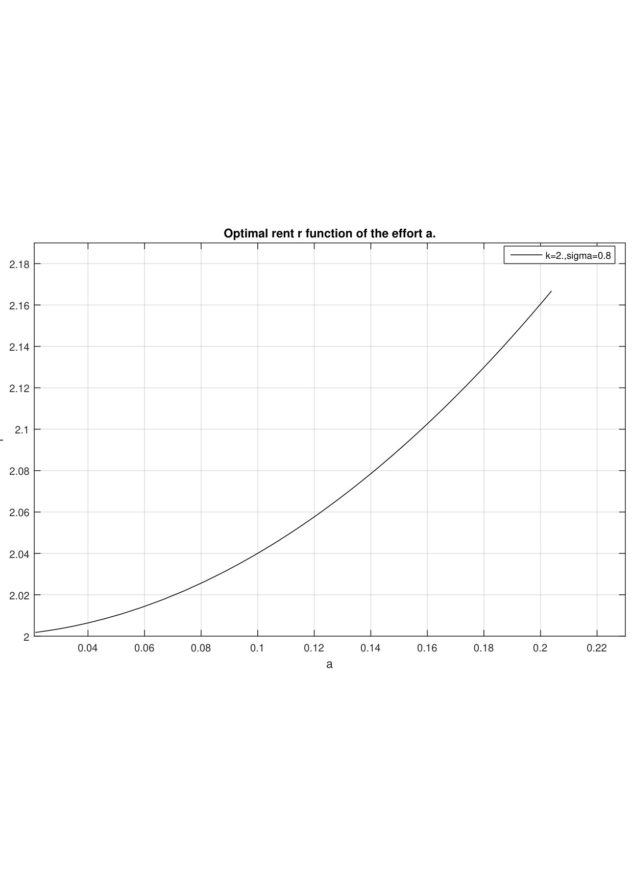 Figure 1
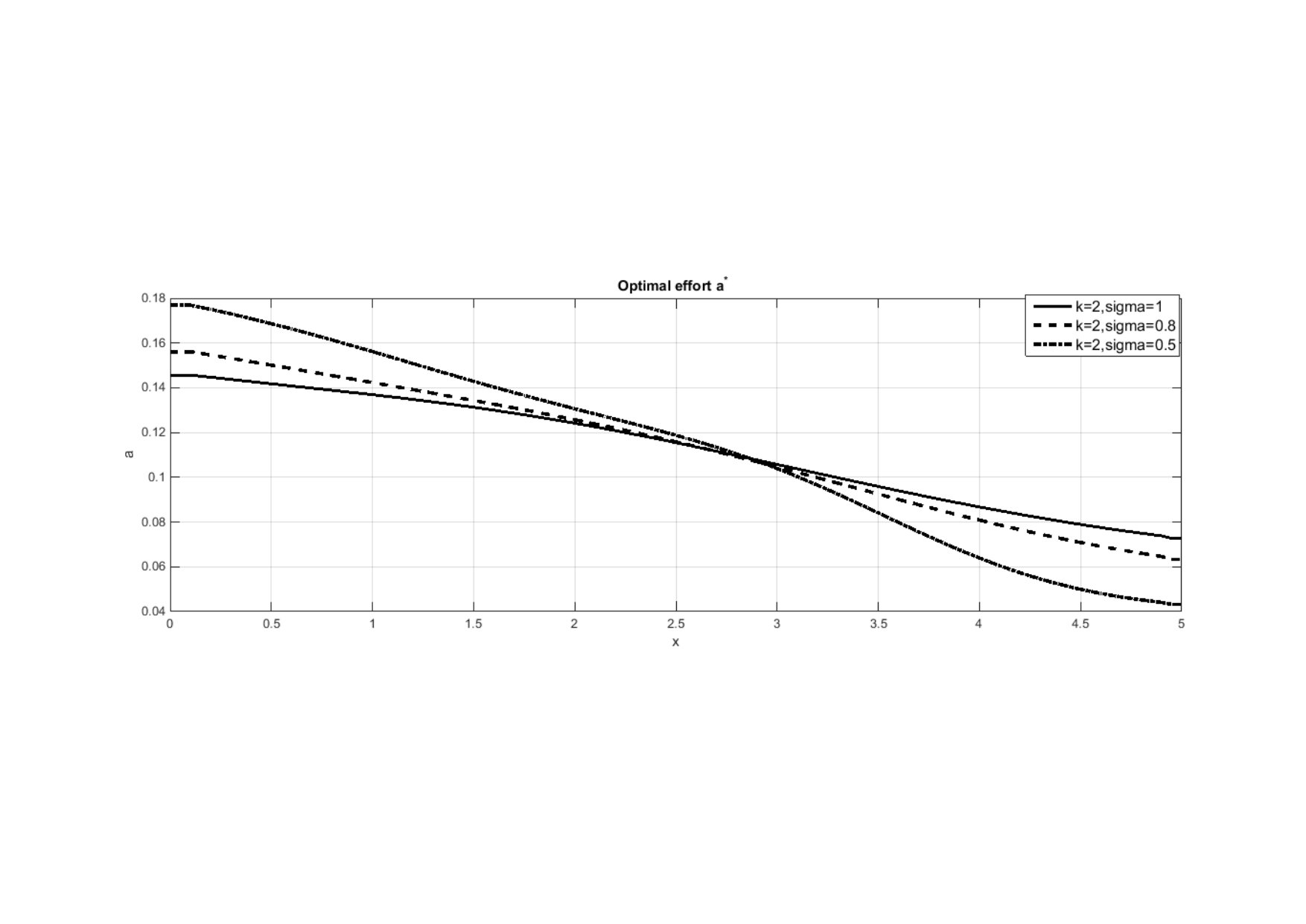 Figure 2
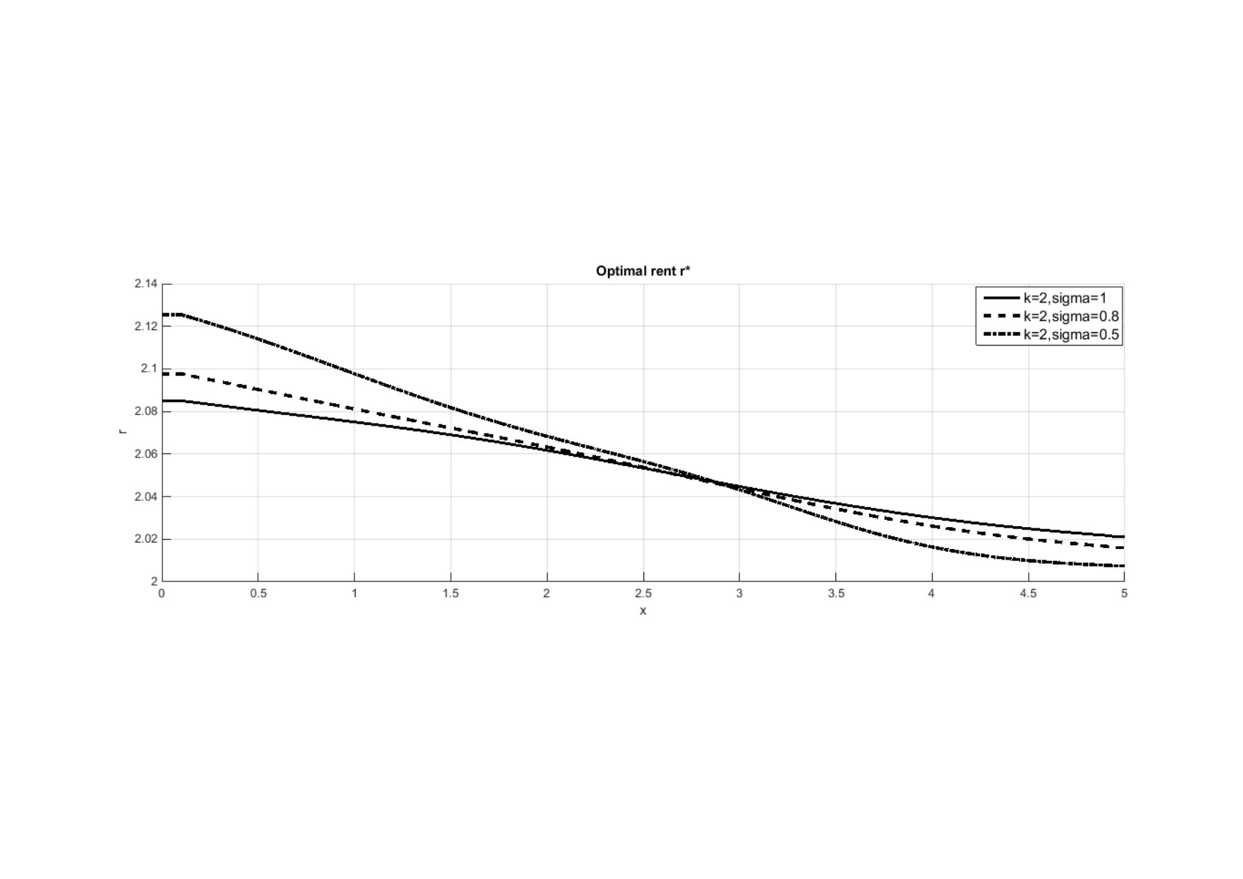 Figure 3
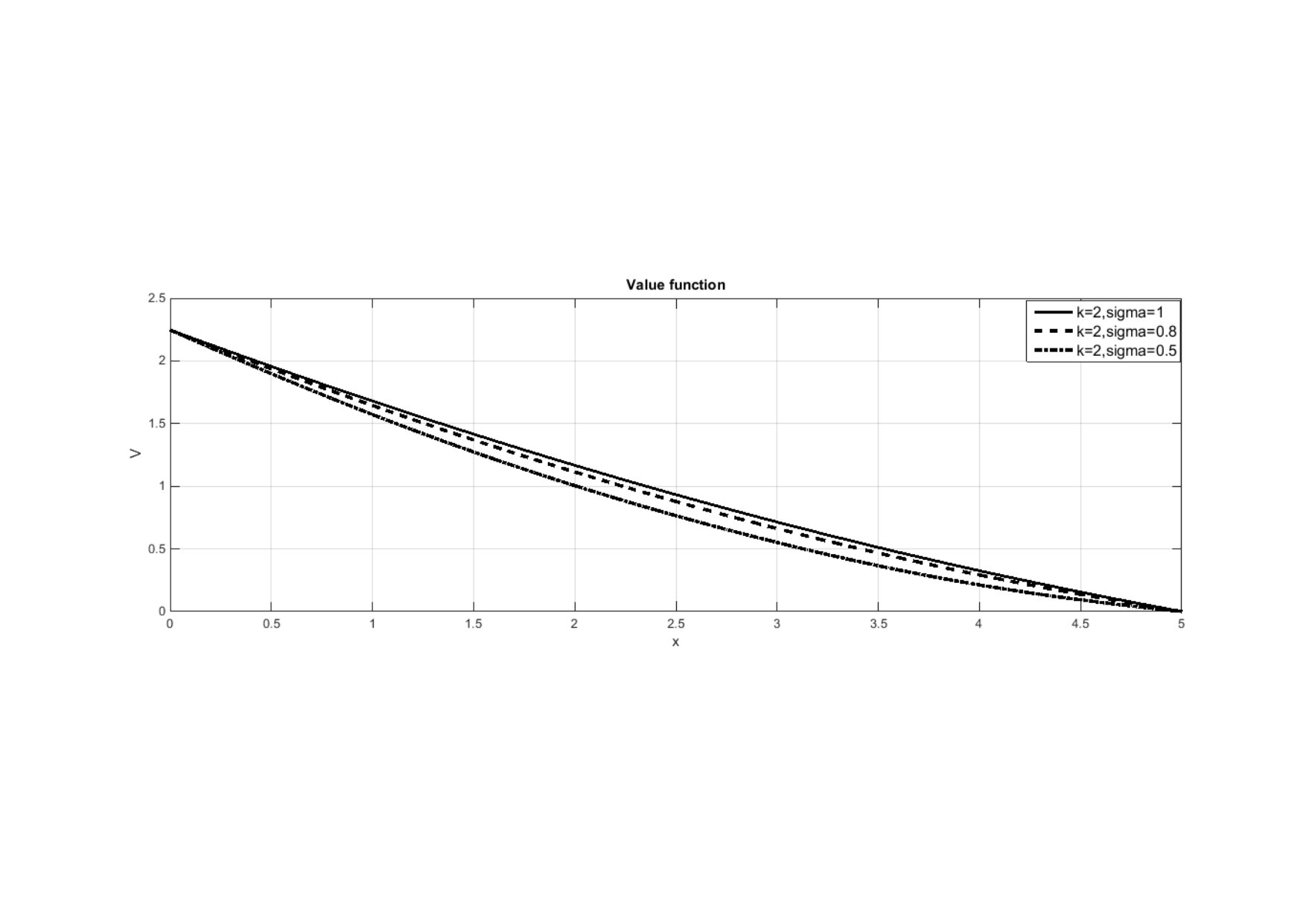 Figure 4
Peer Reviews
No public reviews on file for this paper yet. If you reviewed it on a platform where reviews are public (OpenReview, ICLR, NeurIPS, ICML), you can paste yours below so the community can read it here.
Videos
No videos yet. Explain this paper in a talk, walkthrough, or lecture? Add one.
Taxonomy
TopicsPublic-Private Partnership Projects · Auction Theory and Applications · Transportation Planning and Optimization
Optimal Contract with Moral Hazard for Public Private Partnerships††thanks: We thank Guillaume Carlier, Ivar Ekeland, Dylan Possamaï, Nizar Touzi and Stéphane Villeneuve for interesting and helpful discussions and comments.
Ishak Hajjej , Caroline Hillairet , Mohamed Mnif and Monique Pontier University Tunis Manar, ENIT, LamsinENSAE ParisTech, Crest. The author acknowledges funding from the research programs Chaire Risques Financiers of Fondation du Risque and Investissements d’Avenir (ANR-11-IDEX-0003/Labex Ecodec/ANR-11-LABX-0047). University Tunis Manar, ENIT, Lamsin Institut de Mathématiques de Toulouse
(9 Janvier 2017)
Abstract
Public-Private Partnership (PPP) is a contract between a public entity and a consortium, in which the public outsources the construction and the maintenance of an equipment (hospital, university, prison…). One drawback of this contract is that the public may not be able to observe the effort of the consortium but only its impact on the social welfare of the project. We aim to characterize the optimal contract for a PPP in this setting of asymmetric information between the two parties. This leads to a stochastic control under partial information and it is also related to principal-agent problems with moral hazard. Considering a wider set of information for the public and using martingale arguments in the spirit of Sannikov [18], the optimization problem can be reduced to a standard stochastic control problem, that is solved numerically. We then prove that for the optimal contract, the effort of the consortium is explicitly characterized. In particular, it is shown that the optimal rent is not a linear function of the effort, contrary to some models of the economic literature on PPP contracts.
Keywords : Public Private Partnership, stochastic control under partial information, HJB equation, Moral Hazard.
1 Introduction
A Public Private Parternship contract is defined by the split between private and public tasks concerning a public services, namely: the design of the project, the construction (building), the financing and the maintenance (operate). DBFO means that all the four tasks are supported by the private partner. The goal of PPP contracts is to transfer the risk to the consortium, to provide a better value for money in the use of public funds. In France, by the law of 2008 endorsing the order of 17th June 2004, PPP contract can not be used except if it is expressly justified with regarded to at least one of the following criteria: emergency, complexity, economic efficiency…and actually the conclusion is that almost all projects are in emergency…
The relevance of outsourcing an investment in order to reduce the debt of a public entity has been studied in Espinosa et al. [8]. Here we do not focus on the cost of the construction but on the maintenance aspect of the PPP contract. Hillairet and Pontier propose in [10] a study on PPP and their relevance, assuming the eventuality of a default of the counterparty. In their model, as in other economic papers such as Iossa et al. [11], the rent is assumed to be a linear rule of the effort of the consortium: although this modelisation leads to tractable computations, it seems very ”ad hoc” and economically questionable. The present work does not assume any a priori form for the rent, and in our numerical example, it is shown that the optimal rent is actually not a linear rule.
This paper focuses on the informational asymmetry issue in PPP contracts. Indeed, public and private partners obviously do not share the same information for negotiation, management and follow-up of the contract. Auriol-Picard [1] prove that Build-Operate-Transfer (BOT) contracts (a variant of PPP contracts) may be relevant for the public in case of better information of the private partner, provided a large enough number of concession candidates. But for example in France only three consortium are able to support a PPP contract (Bouygues, Vinci, Eiffage). The support mission of PPP (MAPPP in French, for Mission d’Appui aux PPP), responsible for evaluating the projects in view of legitimate the use of a PPP contract, aims also to reduce the information asymmetry between public entity and consortium. However, as pointed out by the General Inspectorate of Finance in December 2012, the multiple roles of the mission put it ”de facto” in a potential situation of conflict of interest.
Besides, the public may not be able to observe the effort of the consortium, but only its impact on the social welfare of the project. Thus characterizing an optimal PPP contract in this setting of asymmetric information between both partners is related to principal-agent problems with moral hazard. As shown in book of Cvitanic et al. [4], a general theory can be used to solve these problems, by means of forward-backward stochastic differential equations. This work is inspired by the literature on dynamic contracting using recursive methods, and in particular the seminal paper of Sannikov [18] (2008). In Biais et al. [3], the agent is risk-neutral and his efforts, unobservable by the principal, reduce the likelihood of large (but relatively infrequent) losses of the size of a project: more precisely, the losses occur according to a Poisson process whose intensity is controlled by the agent. Pagès and Possamaï [15] propose an optimal contracting between competitive investors and an impatient bank monitoring a pool of long-term loans subject to Markov contagion. The unobservable bank monitoring decision affects the default intensity of an entity of the pool. Optimal contracting in a Brownian setting with risk-averse agent and principal has also been studied recently in Cvitanic et al. [5], by identifying a family of admissible contracts for which the optimal agent’s action is explicitly characterized, and leading to a tractable case for CARA (exponential) utility functions.
In this paper, due to the long maturity of PPP, we consider a perpetual contract between a public entity and a consortium. The consortium supports the initial cost of the project as well as the maintenance costs. The effort that the consortium does to improve the social value of the project is not observable by the public. Thus the rent the public pays to the consortium, to compensate him for his efforts and for the operational costs, is determined on the basis of the public information, that is according to the social value of the project. This is related to principal/agent problem with moral hazard and our approach relies on stochastic control under partial information, as in Bensoussan [2]. We consider a Stackelberg leadership model: the public (the principal) is the leader by offering a contract (characterized by the rent), while the consortium (the agent) gives a best response (characterized by the effort). The aim of this paper is to characterize such optimal contracts. To overcome the difficulty that the control process of the consortium (the effort) is not observable by the public, we restrict the family of admissible contracts to a set of contracts that lead to a tractable characterization of the consortium effort. This could be economically interpreted by the fact that others contracts, for which the public does not know what incentives they will provide to the consortium effort, will likely not be offered. Moreover, we theoretically prove that the optimal contract is indeed of this form. Finally we characterize optimal contracts and provide numerical solutions.
This paper is organized as follows. Section 2 presents the problem, Section 3 provides the solution of this optimal control via Hamilton-Jacobi-Belman equation. Section 4 concludes with numerical illustrations based on the Howard algorithm.
2 Public Private Partnership’s optimal contracts
Throughout the paper, is a filtered probability space, with a Brownian filtration generated by a standard Brownian motion .
2.1 Effort and rent
The operational cost of the project, supported by the consortium (and not observed by the public), is a non-negative -adapted process
[TABLE]
where
- •
is the initial cost of the project, taking into account the construction of the infrastructure.
- •
is the cumulative cost of the project over the period , taking into account both the cost of the construction and the cost of the infrastructure maintenance.
- •
and are respectively the drift and the volatility of the operational cost of the infrastructure maintenance.
Remark 2.1
The cost process is not necessarily non-negative for all Nevertheless, as it is proved in Appendix 5, a sufficient condition to get the cost non-negative on time interval with at least probability is
The consortium supports the operational cost and chooses the effort he does to improve his service for the project : the effort is a non-negative -adapted process , it improves the social value of the project. The social welfare, defined as the social value of the project plus the operational cost, is a -adapted process given by
[TABLE]
where is the initial value of the project (i.e. of the construction, it may be a function of ) and is specified hereafter.
The public observes the social value of the project, but he does not observe directly the effort of the consortium. Thus his information is conveyed by the filtration generated by the social value process . The public chooses the rent he will pay to the consortium to compensate him for his efforts and the operational costs that he supports; the rent is a non-negative -adapted process .
Thus we are looking for optimal control processes with adapted to the filtration generated by the observation but itself is depending on the control process . Remark that in our model the effort only affects the drift and not the volatility of the social welfare (the case of an impact both on the drift and the volatility will be done in a future work). We develop here a strong approach, in the context of stochastic control under partial observation as in Bensoussan [2] Section 2.3.
2.2 A Stackelberg leadership model
We define the respective optimization problems for the consortium and the public. Due to the long maturity of PPP contract (up to 30-50 years), we assume that the contract is perpetual. The public and the consortium have the same time preference parameter . Let us first define the functions involved in the formulation of the optimization problems:
Assumption 2.2
- •
* is the utility function of the consortium, strictly concave strictly increasing and satisfying and Inada’s conditions .*
- •
* models the impact of the consortium’s efforts on the social value, is strictly concave increasing satisfying , (so ), .*
- •
* is the cost of the effort for the consortium; is convex, (thus is increasing) and *
- •
* is convex where *
Finally, the public does not want to pay a rent over a given amount
Remark 2.3
The function is increasing positive, and
We define different sets of admissible contracts, depending on the information flow:
[TABLE]
Those admissibility conditions ensure that entering into the contract provides a non-negative value for the consortium. Remark that in implies the following integrability properties
[TABLE]
We consider a Stackelberg leadership model: the public is the leader by offering a contract (characterized by the rent process ). The consortium gives a best response in terms of the effort process .
**Objective function and continuation value for the consortium and for the public:
**The consortium aims to optimize the expectation of his aggregate utility of the rent minus the drift of the operational cost, minus the cost of his effort
[TABLE]
The public anticipates the consortium’s best response to propose the optimal contract and aims to optimize the expectation of the social welfare minus the rent paid to the consortium
[TABLE]
the last equality being a consequence of the dynamics of the social welfare and the fact that . According to (2.3), the integrals of both objective functions equation (2.4) and equation (2.5) are well defined. From a dynamic point of view, the objective function at time for the consortium is -a.s.
[TABLE]
while the objective function at time for the public is -a.s.
[TABLE]
The consortium chooses the effort and the public chooses the rent in the set of admissible contracts , such as to optimize their respective objective functions, leading to the corresponding continuation value process denoted respectively and .
More precisely, an effort process is incentive compatible with respect to a given rent if it optimizes the consortium’s expected utility (defined in equation (2.4)) given . The problem of the public is to find (the contract) that optimizes his expected discounted profit (defined in equation (2.5)), given the corresponding incentive compatible effort .
Compared to a classic optimization control problem, the difficulty of our formulation is that the public does not observe the control of the consortium, but he observes only its impact on the social value which is the state process of the optimization control problem. The state process appears in an implicit way in the formulation of the optimization problem of the consortium, through the rent process , control of the public. Thus there is no explicit link between the two controls and , the only indirect link involves the state process . The trick to overcome this difficulty is to reformulate the optimization problems in terms of the consortium continuation value process .
2.3 Incentive compatible contract
To encourage the consortium to follow the recommended effort, the public proposes an incentive compatible contract. This subsection characterizes the incentive compatible contracts for in the largest set of admissibility. As in Sannikov [18] or Cvitanic et al. [5] in a weak formulation setting, the following Proposition 2.4 characterizes the dynamics of consortium continuation value process. It is coherent with the result of [5], proved using BSDE’s technics, in a more general framework.
Proposition 2.4
If the contract is incentive compatible, with taking value in with , then the dynamics of the consortium objective function is
[TABLE]
where
[TABLE]
Therefore, , denoted as , realizes the optimal value in (2.6) for the consortium. If is the optimal rent for the public, then the corresponding incentive compatible effort takes value in and the incentive compatible dynamic of the consortium continuation value process is
[TABLE]
Remark 2.5
Incentive compatible contracts imply that the effort is necessarily defined as an adapted process since it has to satisfy where
**Proof: **For any admissible pair let us define the process
[TABLE]
The pair takes its values in the bounded interval Therefore is an -martingale, uniformly integrable, as an -conditional expectation of a bounded random variable: there exists a -predictable process such that and for any :
[TABLE]
The boundedness of implies that the process is uniformly bounded by the integral which goes to [math] when goes to infinity. Thus going to infinity in (2.10) leads to the consortium’s objective value
[TABLE]
Using Definition (2.2)
[TABLE]
The public observes the social value but he could not make difference between the effort and the Brownian motion . The consortium knows that the incentive contract proposed by the public does not optimize the integral . In order to motivate the consortium, the public proposes a contract such that the corresponding optimal effort maximizes the concave function for all , almost everywhere.
It remains to prove that, for the ”optimal” contract, the optimum on of this function is not attained on the bounds of the interval (where is the upper bound of the effort). More precisely, we prove that if the incentive compatible effort is equal to [math] or to , then the public could propose a better contract (that is a rent) that will increase his value function.
Let and be fixed and consider the stochastic set . From the definition of the public continuation value process, on Therefore, on this set, is a constant process. Since the dynamics of the consortium continuation value process follows the uniqueness of the Itô decomposition implies on a.e. On the other hand, on implies However, since the public is the leader, he could propose a rent to the consortium satisfying . The concavity of the functions yields the function is concave. Moreover it satisfies and going to when , thus and . This is a contradiction and . This shows that the incentive compatible effort for the ”optimal” contract satisfies . Similarly .
In the following, all admissible contracts are assumed incentive compatible, and thus are denoted . With a slight abuse of notation we keep the same notations and . In the next section, we will first solve the problem under the set of controls , that is with no restriction of measurability on the rent process. As suggested by Remark 2.5, we will then check that the optimal controls over are functions of the consortium continuation value . Thus equation (2.9) modeling the dynamics of the consortium value function is a Markovian diffusion, the solution of which being defined up to its explosion time We will prove that a.s.
The public value at time [math] over the class is written as follows
[TABLE]
where is the conditional expectation with respect to the event . The fact that the effort is the best response of the consortium, for a given rent , follows from the incentive compatible dynamic (2.9) of the state process .
The next section characterizes, through a HJB equation, the function that realizes the optimum for the public over the class of . But, actually we will prove that the optimal processes over the class are in fact -adapted and the optimal value function for the public over the class is indeed (see Proposition 3.7). Thus we solve ultimately the original optimization problem over the class .
3 Optimal controls and value functions for the public and the consortium
We first solve the optimization problem (2.12) over the set of controls , that is done using the dynamic programming principle. Subsection 3.1 gives a formal derivation of the Hamilton Jacobi Bellman equation
[TABLE]
where the second order differential operator is defined by
[TABLE]
and the control space is defined by
[TABLE]
Subsection 3.2 relates the HJB equation to the optimization problem (2.12), and characterizes the optimal controls and value functions over . We then prove in Subsection 3.3 that the optimal controls over the larger set are actually in .
3.1 Formal derivation of the HJB equation
We assume that the public value function (defined in equation (2.12)) is of class . Standard methods (e.g. El Karoui [7] or Pham [16]) are used to provide the HJB equation that is satisfied by the public value function . We give nevertheless some details for the sake of completeness.
Let and , the dynamic programming principle yields
[TABLE]
Itô’s formula applied to the process and taking expectation yield
[TABLE]
Dividing by letting goes to [math], then using the continuity of the integrands and the mean value theorem we obtain
[TABLE]
Since this holds for any control we obtain the inequality
[TABLE]
On the other hand, suppose that is an optimal control for the class . Then the dynamic programming principle yields
[TABLE]
where is the consortium value function at time , given by the optimal control . By similar arguments, dividing by and sending to [math], one has at time
[TABLE]
which combined with (3.3) yields (3.1).
A useful result to solve this HJB equation is the following.
Lemma 3.1
The function defined in (2.12) is a non-negative bounded function on .
**Proof: **For all and for any , thus Therefore the function is defined on .
For any and due to the concavity of , . Since the function is concave, going from [math] at to when , it admits the maximum
[TABLE]
which bounds from above on . Besides, the constant control is admissible and incentive compatible (the best consortium’s response to a minimum rent is zero effort). Using this control implies that
3.2 Verification theorem
In this subsection the optimal control problem (2.12) is characterized as the solution of the HJB equation (3.1) via a verification theorem (cf. for instance El Karoui [7], Pham [16], Krylov [12] or Fleming-Rishel [9]). The following proposition provides the structure of the optimal control.
Proposition 3.2
*Suppose Assumption 2.2, then there exists a unique admissible optimal pair which realizes the maximum in HJB equation (3.1). This optimal pair is defined by and in the compact interval Moreover, the function is continuous on and is Borel measurable on . *
Example 3.3
*For instance, the hypotheses of Proposition 3.2 are satisfied for: so , The functions and are concave, and is convex. Finally is convex, , , convex yields
In this example, the coefficient of is , so it does not depend on *
**Proof: **(i) Change of variables:
[TABLE]
Recall is non decreasing since is convex and concave. This change of variable is a bijection
[TABLE]
with inverse
[TABLE]
The constraint is the admissibility condition on control
Thus the HJB equation (3.1) is equivalent to
[TABLE]
(ii) For any function and under the hypotheses of Proposition 3.2, the function
[TABLE]
*is strictly concave.
*To prove that is strictly concave, we check that is a positive-definite matrix:
[TABLE]
Computing the first order derivatives:
[TABLE]
Using the concavity of function the second order derivative satisfies
[TABLE]
Other concavity arguments yield
[TABLE]
Finally
[TABLE]
and since , the Jacobian sign is the one of
[TABLE]
which is positive (using again concavity arguments). Then
[TABLE]
and is strictly concave.
(iii) Existence of an optimal pair .
In the HJB equation one has to maximize the function
[TABLE]
When this function is non-increasing and the optimum is
Otherwise, the function is concave and the optimum is achieved for
[TABLE]
Moreover is continuous even at zero points of the function because .
The optimal pair has to satisfy the admissibility condition
[TABLE]
Since the function
[TABLE]
is continuous on the compact interval there exists an optimal solution . Moreover by a selection theorem (See Appendix B, Fleming and Rishel [9]), there exists a Borel-measurable function from into . Finally, by construction takes its values in .
Proposition 3.4
*Define and suppose Assumption 2.2. Then
(i) The consortium initial value is in the interval .
(ii) *
**Proof: **i) We assume and we prove that it leads to a contradiction. Let and define the strict convex function . Then , increasing and decreasing imply that . For any control , one has by strict concavity of the function
[TABLE]
and by strict convexity of , with our choice of , ,
[TABLE]
For any control that is not identical to ,
[TABLE]
where the last inequality holds from (3.6) and (3.7). Since , for ,
[TABLE]
By taking the supremum over all admissible strategies, we get
[TABLE]
On the other hand, by Lemma 3.1, one has . This gives a contradiction to (3.9), and is necessarily smaller than .
ii) We now prove that .
The proof follows the same lines as the previous part with this time .
We notice that the constant control , which leads to , is an admissible control and so the equality makes sense. Let us recall that , . For any control , one has by concavity of the function
[TABLE]
and by convexity of
[TABLE]
thus
[TABLE]
and implies
[TABLE]
Taking the supremum over all incentive compatible admissible strategies, we get
[TABLE]
Besides by Lemma 3.1. Therefore .
Lemma 3.5
The function satisfies
[TABLE]
**Proof: **Since every admissible control must satisfy , then the equality holds for every control satisfying which is equivalent to
[TABLE]
In this class of controls, one has
[TABLE]
This shows that
[TABLE]
and the equality holds when a.e. where realizes the maximum of the function on and . We easily check that the control is indeed admissible (incentive compatible). This proves (3.11).
We now proceed to the verification Theorem (cf. [16] Th. 3.5.3., infinite horizon). Thanks to Proposition 3.4 and Lemma 3.5, we study the HJB equation on a bounded domain with the Dirichlet boundary conditions
[TABLE]
Theorem 3.6
Under Assumption 2.2 the HJB equation (3.1) with boundary conditions (3.12) admits a unique solution in . Let be the argmax in the HJB equation (3.1). We assume that is of bounded variation, then the associated stochastic differential equation
[TABLE]
*admits a unique strong solution denoted as We define the following controls:
almost everywhere. Then, is the optimal control in . As a conclusion, the public value function satisfies *
Remark that on the numerical simulations, is decreasing and thus is indeed of bounded variation.
Proof: Step 1: The equation (3.1) admits an unique solution.
This follows from Theorem 1 in [19], whose assumptions are satisfied. Indeed the set of controls is a nonempty compact set. The coefficients of the HJB equation (3.1) are affine functions of the variable , and continuous functions in the control , for each , thus standard linear growth assumptions on the coefficients of (3.1) are satisfied. Under Assumption 2.2, the function is increasing positive, and . Therefore the volatitity coefficient of the HJB equation (3.1) admits a uniform lower bound. In addition, the coefficient is bounded on . Therefore, applying Theorem 1 in [19], the HJB equation (3.1) has a twice continously differentiable solution in , and continuous on .
Furthermore Proposition 3.2 proves that for all there exists an admissible pair in such that
[TABLE]
Step 2:
Let and the corresponding process with dynamic
[TABLE]
Applying Itô’s formula to the process
[TABLE]
with being a bounded process. Taking the expectation, for all
[TABLE]
From the HJB equation (3.1), thus
[TABLE]
Using boundedness from above of when (cf. the proof of Lemma 3.1) and admissibility conditions on , one has . By the dominated convergence theorem, we obtain
[TABLE]
Besides, as is a continuous function and is bounded, one has
[TABLE]
Therefore
[TABLE]
so for any we get
[TABLE]
and
[TABLE]
Step 3: the SDE (3.13) admits a unique strong solution
Let us consider the SDE (3.13) associated to the optimal pair , then , a.e. satisfies the SDE
[TABLE]
The existence of a strong solution of this SDE is given by Nakao [14] (Theorem p. 516), as the drift is bounded measurable, the volatility is strictly bounded from below and of bounded variation (since it is the case for ). The existence of a strong solution of the SDE (3.13) follows.
Step 4:
This solution actually is the process denoted as meaning where . We now repeat the above arguments of Step 2:
[TABLE]
Thus for and all
[TABLE]
But since satisfies the HJB equation (3.1) with such optimal controls we get
[TABLE]
[TABLE]
Taking into account the boundedness of the controls (cf. Proposition 3.2), the dominated convergence theorem allows us to get and going to infinity in . Besides, Fatou’s lemma and boundedness of allow us to get and going to infinity in . Therefore
[TABLE]
Conclusion: is the public value function defined in equation (2.12) and is a Markovian optimal control.
3.3 Going back to the original set of control processes
In this subsection, we will prove that the process is -adapted.
Proposition 3.7
Under the assumptions of Theorem 3.6, the unique strong solution to the stochastic differential equation (3.13) admits an infinite explosion time, and the filtrations , and coincide at the optimum.
**Proof: **First, as and are bounded, the strong solution of the SDE (3.13) does not explode. Besides, and are obviously included in .
(i) We first express as the solution of the SDE (3.13)
[TABLE]
Under the assumptions of Theorem 3.6, this SDE admits an unique strong solution, thus the filtrations generated by and coincide since the coefficient of is positive (cf. Corollary 1.12 of Revuz-Yor [17]).
(ii) On the other hand, by definition:
[TABLE]
thus, since
[TABLE]
and
[TABLE]
Once again, under the assumptions of Theorem 3.6, is a strong solution of this stochastic differential equation driven by so this process is -adapted. Therefore the three filtrations , and coincide at the optimum.
4 Numerical implementation
The consortium continuation value is the state parameter used in the resolution of the stochastic control problem of Section 3. Proposition 3.4 gives an upper bound for the consortium initial value .
4.1 Howard’s Algorithm
The HJB-equation (3.1) is written as follows
[TABLE]
Let be the finite difference step on the state coordinate and , , be the points of the grid The equation (4.1) is discretized by replacing the first and second derivatives of with the following approximations
[TABLE]
[TABLE]
[TABLE]
where .
This leads to the system of equations with unknowns :
[TABLE]
where is given by
[TABLE]
the matrix is defined as follows:
[TABLE]
with , and
[TABLE]
To solve the latter equation we use an iterative Howard algorithm (cf. Howard [13] chapter 8). It consists in computing two sequences and (starting from chosen arbitrary):
step : to the strategy we compute solution of the linear system
[TABLE]
on the grid
step : is associated with a strategy
[TABLE]
The convergence of the Howard algorithm holds when the matrix satisfies the discrete maximum principle: a sufficient condition is that is diagonally dominant. This is the case since .
4.2 Effort and rent
We recall
and
in the compact interval .
If in the compact interval
If in the compact interval
4.3 Numerical results
In this section we choose and the functions of the example 3.3 : so
We choose the parameter We restrict our figures to (cf. Proposition 3.4), that is in our numerical example.
In Figure 2, Figure 3 and Figure 4, and varies : or . Figure 1 gives the optimal rent function of the optimal effort, for and .
We observe that and are non-increasing functions of the consortium value.
4.3.1 Graph of the optimal rent as a function of
The more interesting observation is that the optimal rent is an increasing convex function of the optimal effort. This contradicts the usual assumption of linear dependence between rent and effort. Besides, the qualitative behaviour of these optimal parameters is the same with respect to both and
4.3.2 Sensibility of the results to parameter
According to Figure 2, it seems that the optimal public value function is increasing with respect to : the risk is supported by the consortium. The same behavior is observed for the optimal effort (Figure 3) and for the optimal rent (Figure 4) in case of large enough. But, when is lower the optimal effort is decreasing. In case of a low level of the private continuation value , the consortium is not ready to provide more efforts. This behavior is observed for any parameter
4.3.3 Sensibility of the results to parameter
Actually, the true parameter control is , so, as it could be expected, the parameter has no impact on the behaviors of and
Conclusion
This paper provides a characterisation of optimal public private partnership contracts in a moral hazard framework, using martingale methods and stochastic control. A numerical example shows that, in particular, the optimal rent is a convex (and not linear) function of the effort. This convexity, due to the information asymmetry between the consortium and the public entity, implies for the public entity a more and more costly contract to encourage the consortium to do more efforts. This feature should be taken into account in the models concerning PPP contracts.
5 Appendix A
We need to know some sufficient conditions to get the cost process non-negative on a time interval . Recall the Inverse Gaussian law with density on
[TABLE]
The cost process is a drifted Brownian motion and the event
[TABLE]
where is an hitting time. It is well known (cf. [6] for instance) that the law of is meaning that we would like to bound with (for instance)
[TABLE]
After the change of variable , since this probability is bounded by
[TABLE]
where is the distribution function of the standard Gaussian law. A sufficient condition to get the cost non-negative on time interval with at least probability is
[TABLE]
The reference list from the paper itself. Each links out to its DOI / PubMed record.
- 1[1] E. Auriol, P.M. Picard. A theory of BOT concession contracts. Journal of of Economic Behaviour and Organization, 2834 , (2011).
- 2[2] A. Bensoussan. Stochastic control of partially observable systems, Cambridge University Press , (1992).
- 3[3] B. Biais, T. Mariotti, J.C. Rochet, S. Villeneuve. Large risks, limited liability and dynamic moral hazard. Econometrica , Vol. 78, No. 1 (January, 2010), 73–118.
- 4[4] J. Cvitanic, J. Zhang. Contract Theory in Continuous-Time Models, Springer (2013).
- 5[5] J. Cvitanic, D. Possamaï, N. Touzi. Moral hazard in dynamic risk management, arxiv:1510.07111 (2015).
- 6[6] M. Chesney, M. Jeanblanc, M. Yor. Mathematical Methods for Financial Markets, Springer (2009).
- 7[7] N. El Karoui. Les aspects probabilistes du contrôle stochastique, Saint Flour 1979, Volume 876 of Lectures Notes In Math. (1981).
- 8[8] G.E. Espinosa, C. Hillairet, B. Jourdain, M. Pontier. Reducing the debt: Is it optimal to outsource an investment? (2016). a voir To appear in Mathematics and Financial Economics.