
TL;DR
This paper introduces an algorithm to analyze cosmological implications of various quantum field theories using soft attractors, focusing on scalar fields and their correlation functions within modified gravity frameworks, with results consistent with observations.
Contribution
It develops a comprehensive framework for studying cosmological effects of scalar fields in modified gravity, including exact correlation function computations and new consistency relations.
Findings
Explicit calculations of two, three, and four point correlation functions.
Theoretical bounds on primordial power spectrum parameters.
Identification of deviations from canonical slow roll models.
Abstract
In this work, we have developed an elegant algorithm to study the cosmological consequences from a huge class of quantum field theories (i.e. superstring theory, supergravity, extra dimensional theory, modified gravity etc.), which are equivalently described by soft attractors in the effective field theory framework. In this description we have restricted our analysis for two scalar fields - dilaton and Higgsotic fields minimally coupled with Einstein gravity, which can be generalized for any arbitrary number of scalar field contents with generalized non-canonical and non-minimal interactions. We have explicitly used gravity, from which we have studied the attractor and non-attractor phase by exactly computing two point, three point and four point correlation functions from scalar fluctuations using In-In (Schwinger-Keldysh) and formalism. We have also presented…
Click any figure to enlarge with its caption.
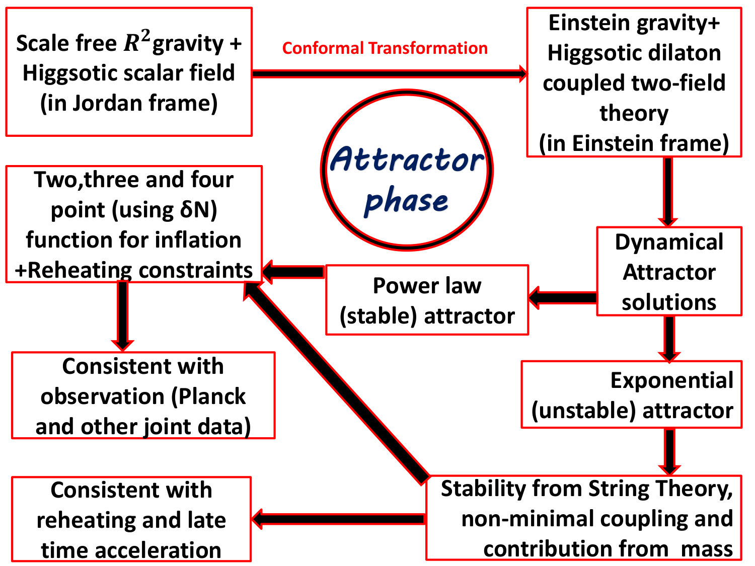 Figure 1
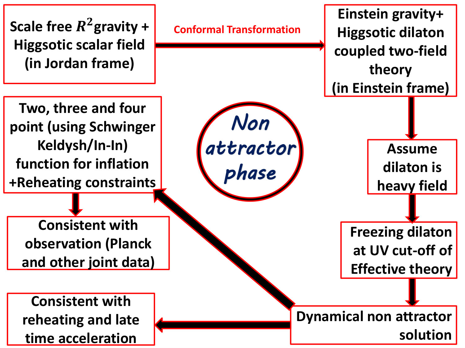 Figure 2
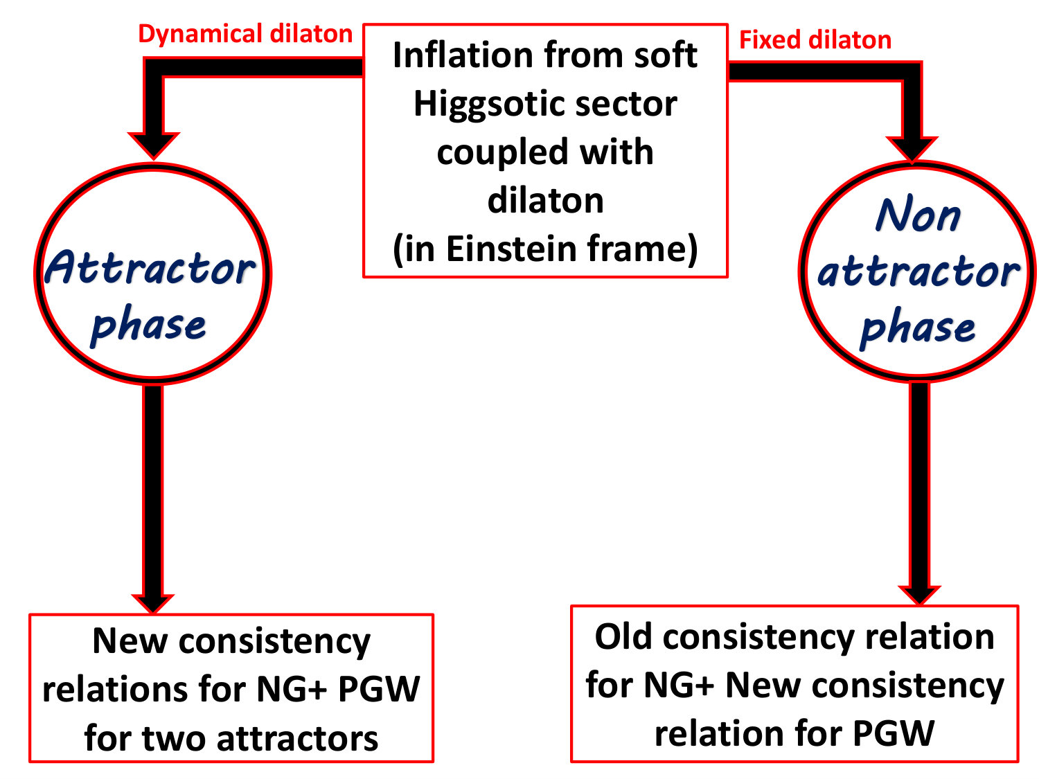 Figure 3
 Figure 4
 Figure 5
 Figure 6
 Figure 7
 Figure 8
 Figure 9
 Figure 10
 Figure 11
 Figure 12
 Figure 13
 Figure 14
 Figure 15
 Figure 16
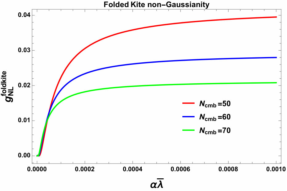 Figure 17
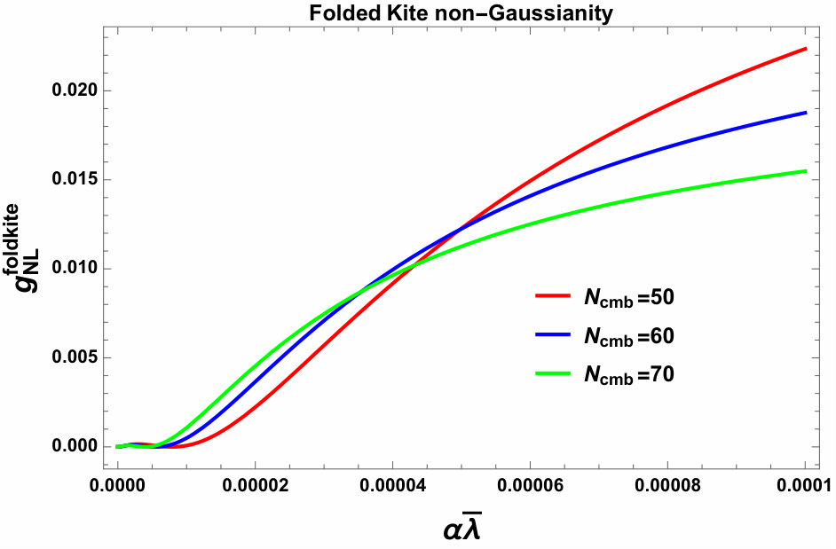 Figure 18
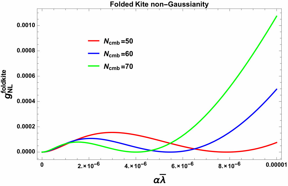 Figure 19
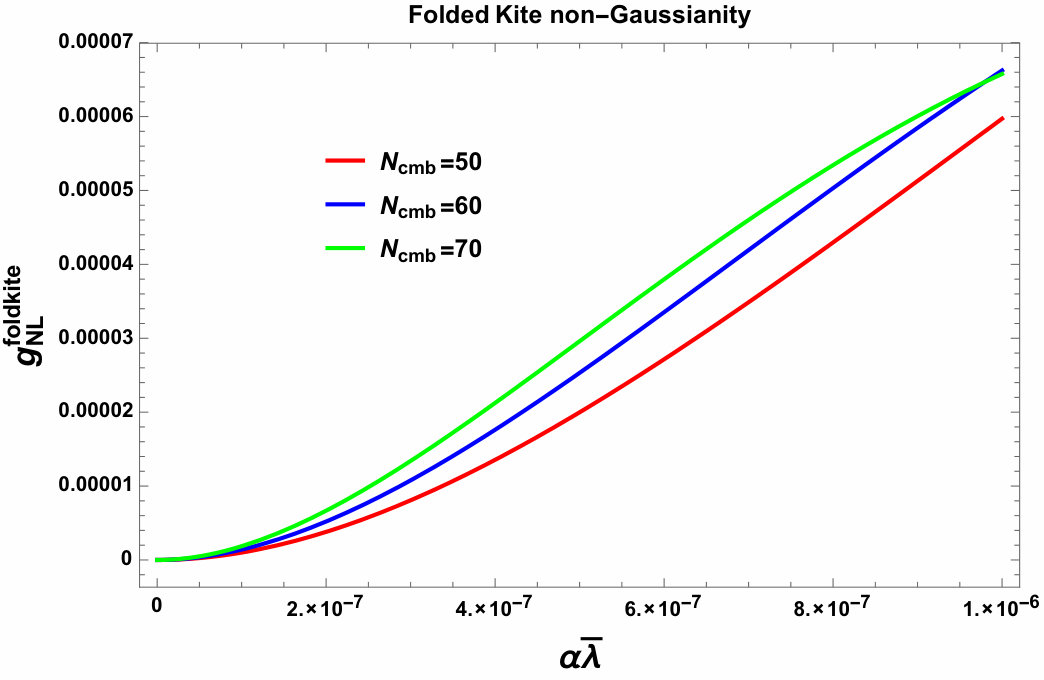 Figure 20
 Figure 21
 Figure 22
 Figure 23
 Figure 24
 Figure 25
 Figure 26
 Figure 27
 Figure 28
 Figure 29
 Figure 30
 Figure 31
 Figure 32
 Figure 33
 Figure 34
 Figure 35
 Figure 36
 Figure 37
 Figure 38
 Figure 39
 Figure 40
| () | () | () | ||
|---|---|---|---|---|
| Case I Case II | Case I Case II | Case I Case II | Case I Case II | |
| 50 | 0.941 0.940 | 1.16 1.20 | -4.56 -4.80 | |
| 60 | 2.2 2.3 | 0.951 0.950 | 0.80 0.83 | -2.61 -2.76 |
| 70 | 0.958 0.957 | 0.59 0.62 | -1.65 -1.78 |
| (in ) | (in ) | (in ) | (in ) | (in ) | |||||
|---|---|---|---|---|---|---|---|---|---|
| 50 | 60 | 51 | 14.1 | 15.5 | 1.4 | ||||
| 60 | 70 | 61 | 10 | 9 | 15.5 | 16.7 | 2 | 1.2 | |
| 70 | 80 | 71 | 16.7 | 17.9 | 1.2 |
| (in ) | (in ) | (in ) | (in ) | (in ) | (in ) | |||
|---|---|---|---|---|---|---|---|---|
| 50 | 0.94 | 1.2 | -4.8 | |||||
| 60 | 2.207 | 0.95 | 0.8 | -2.8 | ||||
| 70 | 0.96 | 0.6 | -1.8 |
| Scanning Region | Bound on | ||
|---|---|---|---|
| I | |||
| II | |||
| III | |||
| IV | |||
| I+II+III+IV |
| Scanning Region | ||
|---|---|---|
| I | ||
| II | ||
| III | ||
| IV | ||
| I+II+III+IV |
| Scanning Region | ||
|---|---|---|
| I | ||
| II | ||
| III | ||
| IV | ||
| I+II+III+IV |
Peer Reviews
No public reviews on file for this paper yet. If you reviewed it on a platform where reviews are public (OpenReview, ICLR, NeurIPS, ICML), you can paste yours below so the community can read it here.
Videos
No videos yet. Explain this paper in a talk, walkthrough, or lecture? Add one.
TIFR/TH/16-50
aainstitutetext: Department of Theoretical Physics, Tata Institute of Fundamental Research, Colaba, Mumbai - 400005, India
COSMOS-- soft Higgsotic attractors
Sayantan Choudhury 111**Presently working as a Visiting (Post-Doctoral) fellow at DTP, TIFR, Mumbai,
Alternative E-mail: [email protected]**.
Abstract
In this work, we have developed an elegant algorithm to study the cosmological consequences from a huge class of quantum field theories (i.e. superstring theory, supergravity, extra dimensional theory, modified gravity etc.), which are equivalently described by soft attractors in the effective field theory framework. In this description we have restricted our analysis for two scalar fields - dilaton and Higgsotic fields minimally coupled with Einstein gravity, which can be generalized for any arbitrary number of scalar field contents with generalized non-canonical and non-minimal interactions. We have explicitly used gravity, from which we have studied the attractor and non-attractor phase by exactly computing two point, three point and four point correlation functions from scalar fluctuations using In-In (Schwinger-Keldysh) and formalism. We have also presented theoretical bounds on the amplitude, tilt and running of the primordial power spectrum, various shapes (equilateral, squeezed, folded kite or counter collinear) of the amplitude as obtained from three and four point scalar functions, which are consistent with observed data. Also the results from two point tensor fluctuations and field excursion formula are explicitly presented for attractor and non-attractor phase. Further, reheating constraints, scale dependent behaviour of the couplings and the dynamical solution for the dilaton and Higgsotic fields are also presented. New sets of consistency relations between two, three and four point observables are also presented, which shows significant deviation from canonical slow roll models. Additionally, three possible theoretical proposals have presented to overcome the tachyonic instability at the time of late time acceleration. Finally, we have also provided the bulk interpretation from the three and four point scalar correlation functions for completeness.
Keywords:
Cosmology beyond the standard model, De Sitter space, String Cosmology, Modified gravity.
1 Introduction
The inflationary paradigm is a theoretical proposal which attempts to solve various long-standing issues with standard Big Bang Cosmology and has been studied earlier in various works Guth:1980zm ; Baumann:2009ds ; Senatore:2016aui ; Liddle:1999mq ; Langlois:2010xc ; Riotto:2002yw ; Lyth:1998xn ; Lyth:2007qh ; Weinberg:2003sw ; Weinberg:2008hq ; Cheung:2007st ; Bardeen:1980kt . But apart from the success of the this theoretical framework it is important to note that there is no single model exists till now using which one can explain the complete evolution history of the universe and also unable to break the degeneracy between various cosmological parameters computed from various models of inflation Choudhury:2011sq ; Choudhury:2011jt ; Choudhury:2012yh ; Choudhury:2012ib ; Choudhury:2013zna ; Choudhury:2013jya ; Choudhury:2014sxa ; Choudhury:2015pqa ; Choudhury:2014hja ; Choudhury:2016wlj ; Choudhury:2015hvr ; Bhattacharjee:2014toa ; Deshamukhya:2009wc ; Kachru:2003sx ; Kachru:2003aw ; Iizuka:2004ct ; Choudhury:2014kma ; Choudhury:2013iaa ; Choudhury:2013woa ; Choudhury:2014sua ; Choudhury:2014wsa . It is important to note that, the vacuum energy contribution generated by the trapped Higgs field in a metastable vacuum state which mimics the role of effective cosmological constant in effective theory. At the later stages of Universe such vacuum contribution dominates over other contents and correspondingly Universe expands in a exponential fashion. But using such metastable vacuum state it is not possible to explain the tunneling phenomena and also impossible to explain the end of inflation. To serve both of the purposes shape of the effective potential for inflation should have flat structure. Due to such specific structure effective potential for inflation satisfy flatness or slow-roll condition using which one can easily determine the field value corresponding to the end of inflation. There are various classes of models exists in cosmological literature where one can derive such specific structure of inflation Choudhury:2011jt ; BuenoSanchez:2006rze ; Allahverdi:2006iq ; Ross:1995dq ; Allahverdi:2006rt ; Enqvist:2003gh ; Allahverdi:2006we . For an example, the Coleman-Weinberg effective potential serves this purpose Coleman:1973jx ; Barenboim:2013wra . Now if we consider the finite temperature contributions in the effective potential Fodor:1994bs ; Quiros:1999jp then such thermal effects need to localize the inflaton field to small expectation values at the beginning of inflation. The flat structure of the effective potential for inflation is such that the scalar inflaton field slowly rolls down in the valley of potential during which the scale factor varies exponentially and then infation ends when the scalar inflaton field goes to the non slow-rolling region by violating the flatness condition. At this epoch inflaton field evolves to the true minimum very fast and then it couples to the matter content of the Universe and reheats our Universe via subsequent oscillations about the minimum of the slowly varying effective potential for inflation. These class of models are very successful theoretical probe through which it is possible to explain the characteristic and amplitude of the spectrum of density fluctuations with high statistical accuracy ( CL from Planck 2015 data Ade:2015lrj ; Ade:2015ava ; Ade:2015xua ) and at late times this perturbations act as the seeds for the large scale structure formation, which we observe at the present epoch. Apart from this huge success of inflationary paradigm in slowly varying regime it is important to mention that, these density fluctuations generated from various class of successful models were unfortunately large enough to explain the physics of standard Grand Unified Theory (GUT) with well known theoretical frameworks and also it is not possible to explain the observed isotropy of the Cosmic Microwave Background Radiation (CMBR) at small scales during inflationary epoch. The only physical possibility is that the self interactions of the inflaton field and the associated couplings to other matter field contents would be sufficiently small for which it is possible to satisfy these cosmological and particle physics constraints. But the prime theoretical challenge at this point is that for such setup it is impossible to achieve thermal equilibrium at the end of inflation. Consequently, it is not at all possible to localize the scalar inflaton field near zero Vacuum Expectation Value (VEV), where is the corresponding vacuum state in quasi de Sitter space time. Therefore, a sufficient amount of expansion will not be obtained from this prescribed setup. Here it is important to note that, for a broad category of effective potentials the inflaton field evolves with time very slowly compared to the Hubble scale following slow-roll conditions and satisfies all of the observational constraints Ade:2015lrj ; Ade:2015ava ; Ade:2015xua computable from various inflationary observables from this setup. However, apart from the success of slow roll inflationary paradigm the density fluctuations or more precisely the scalar component of the metric perturbations restricts the coupling parameters to be sufficiently small enough and allows huge fine-tuning in the theoretical set up. This is obviously a not recommendable prescription from model builder’s point of view. Additionally, all of these class of models are not ruled out completely by the present observed data (Planck 2015 and other joint data sets Ade:2015lrj ; Ade:2015ava ; Ade:2015xua ; Ade:2015tva ), as they are degenerate in terms of determination of inflationary observables and associated cosmological parameters in precision cosmology. There are various ideas exist in cosmological literature which can drive inflation. These are appended below:
- •
Category I:
In this class of models, inflation drives through a field theory which involves a very high energy physics phenomena. Example: string theory and its supergravity extensions Choudhury:2016wlj ; Choudhury:2015hvr ; Choudhury:2014sxa ; Choudhury:2013zna ; Choudhury:2012ib ; Choudhury:2012yh ; Choudhury:2011sq ; Yamaguchi:2011kg ; Stewart:1994ts ; McAllister:2007bg ; Baumann:2009ni ; Nilles:1983ge ; Linde:1997sj ; BasteroGil:2006cm ; Choudhury:2011rz ; Alishahiha:2004eh ; Silverstein:2016ggb ; Flauger:2014ana ; McAllister:2014mpa ; Silverstein:2013wua ; Silverstein:2008sg ; Panda:2010uq ; Panda:2007ie ; Mazumdar:2001mm ; Choudhury:2002xu ; Choudhury:2003vr ; Deshamukhya:2009wc ; Choudhury:2015baa ; Choudhury:2015fzb ; Choudhury:2016rtp ; Maharana:1997cz ; Headrick:2004hz ; Minwalla:2003hj ; David:2001vm ; Gopakumar:2000rw ; Sen:2000kd ; Rastelli:2000hv ; Sen:2002qa ; Sen:2002in ; Sen:2002an ; Sen:1999xm ; Sen:2002nu ; Mandal:2003tj , various supersymmetric models Choudhury:2011jt ; BuenoSanchez:2006rze ; Allahverdi:2006iq ; Ross:1995dq ; Allahverdi:2006rt ; Enqvist:2003gh ; Allahverdi:2006we etc.
- •
Category II:
In this case, inflation is driven by changing the mathematical structure of the gravitational sector. This can be done using the following ways:
Introducing higher derivative terms of the form of , where is the Ricci scalar Starobinsky:1979ty ; Sebastiani:2015kfa ; DeFelice:2010aj ; Sotiriou:2008rp . Example: Starobinsky inflationary framework which is governed by the model Starobinsky:1979ty , , where the coefficients and are given by, and . If we set and then we can get back the theory of scale free gravity in this context. In this paper will we explore the cosmological consequences from scale free theory of gravity. 2. 2.
Introducing higher derivative terms of the form of Gauss Bonnet gravity coupled with scalar field in non-minimal fashion, where the contribution in the effective action can be expressed as Kanti:2015pda ; Nozari:2008ny ,
[TABLE]
where is the inflaton dependent coupling which can be treated as the non-minimal coupling in the present context. This is also an interesting possibility which we have not explored in this paper. Here one cannot consider the Gauss Bonnet term in the gravity sector in 4D without coupling to other matter fields as in 4D Gauss Bonnet term is topological surface term. 3. 3.
Another possibility is to incorporate the effect of non-minimal coupling of inflaton field and the gravity sector Bezrukov:2007ep ; Hertzberg:2010dc ; Pallis:2010wt . The simplest example is, gravity theory. For Higgs inflation Bezrukov:2007ep ,, where is the non-minimal coupling of the Higgs field. Here one can consider more complicated possibility as well by considering a non-canonical interaction between inflaton and gravity by allowing term in the 4D effective action Budhi:2017yjd . For the construction of effective potential we have considered this possibility. 4. 4.
One can also consider the other possibility, where higher derivative non-local terms can be incorporated in the gravity sector Modesto:2011kw ; Biswas:2011ar ; Biswas:2012ka ; Biswas:2012bp ; Biswas:2013cha ; Talaganis:2014ida ; Biswas:2014tua ; Modesto:2014lga ; Dona:2015tra ; Koshelev:2016xqb . For example one can consider the possibilities, , , , ,, , , where is defined as, is the d’Alembertian operator in 4D and the are analytic entire functions containing higher derivatives up to infinite order. This is itself a very complicated possibility which we have not explored in this paper.
- •
Category III:
In this case, inflation is driven by changing the mathematical structure of both the gravitational and matter sector of the effective theory. One of the examples is to use Jordan-Brans-Dicke (JBD) gravity theory Brans:1961sx ; Brans:1962zz along with extended inflationary models which includes non-canonical interactions. By adjusting the value of Brans-Dicke parameters one can study the observational consequences from this setup. Instead of Jordan-Brans-Dicke (JBD) gravity theory one can also use non local gravity or many other complicated possibilities.
In this paper, we consider the possibility of soft inflationary paradigm in Einstein frame, where a chaotic Higgsotic potential is coupled to a dilaton via exponential type of potential, which is appearing through the conformal transformation from Jordan to Einstein frame in the metric within the framework of scale free gravity. Here it is important to mention that, in case of soft inflationary model, the dilaton exponential potential is multiplied by an coupling constant of the Higgsotic theory which mimics the role of an effective coupling constant and its value always decreases with the field value. One can generalize this idea for any arbitrary matter interactions which is also described by generalized theory Chen:2006nt ; Khoury:2010gb (see appendix 10.1 for more details). In this context of discussion also it is important to specify that, one can treat the field dependent couplings in the simple effective potentials or may be in a generalized functionals contains a decaying behaviour with dilaton field value as it contains an overall exponential factor which is coming from the dilaton potential itself in Einstein frame. This is a very interesting feature from the point of view of RG flow in QFT as the field dependent coupling in Einstein frame captures the effect of field flow (energy flow). In this context instead of solving directly the RGE for the effective coupling, we solve the dynamical equations for the fields and the effective coupling for power law and exponential attractors. Due to the similarities in both of the techniques here one can arrive at the conclusion that in cosmology solving a dynamical attractor problem in presence of effective coupling in Einstein frame mimics the role of solving RGE in QFT. Thus due to the exponential suppression in the effective coupling in Einstein frame it is naturally expected from the prescribed framework that for suitable choices of the model parameters soft cosmological constraints can be obtained Berkin:1990ju ; Berkin:1991nm . As in this prescribed framework dilaton exponential coupling plays very significant role, one can ask a very crucial question about its theoretical origin. Obviously there are various sources exist from which one can derive exponential effective couplings or more precisely the effective potentials for dilaton. These possibilities are appended bellow:
- •
Source I**:
**One of the source for dilaton exponential potential is string theory, which is appearing in the Category I. Specifically, superstring theory and low energy supergravity models are the theoretical possibilities in string theory Bars:1992sr ; Callan:1985ia ; Bars:1990rb ; Choudhury:2013yg ; Choudhury:2013aqa ; Choudhury:2014hna ; Choudhury:2015wfa ; Derendinger:1985kk ; Ellis:1986zt ; Pilch:2000ue where dilaton exponential potential is appearing in the gravity part of the action in Jordan frame and after conformal transformation in Einstein frame such dilaton effective potential is coupled with the matter sector. The most important example is -attractor which mimics a class of inflationary models in supergravity in 4D. For details see ref. Kallosh:2013yoa ; Kallosh:2014rga ; Galante:2014ifa ; Kallosh:2015lwa ; Linde:2015uga ; Carrasco:2015uma ; Carrasco:2015rva ; Carrasco:2015pla ; Kallosh:2016gqp ; Kallosh:2016sej ; Ferrara:2016fwe .
- •
Source II**:
**Another possible source of dilaton exponential potential is coming from modified gravity theory framework such as, gravity Starobinsky:1979ty ; Sebastiani:2015kfa ; DeFelice:2010aj ; Sotiriou:2008rp , gravity Bezrukov:2007ep ; Hertzberg:2010dc ; Pallis:2010wt ; Budhi:2017yjd and Jordan-Brans-Dicke theory Brans:1961sx ; Brans:1962zz in Jordan frame, which are appearing in the Category II (1& 3) and Category III. After transforming the theory in the Einstein frame via conformal transformation one can derive dilaton exponential potential.
In fig (1(a)), fig (1(b)) and fig (1(c)), we have shown the diagrammatic representation of attractor and non-attractor phase of soft Higgsotic inflation. In these representative diagrams we have shown the steps followed during the computation.
In this work we have addressed the following important points through which it is possible to understand the underlying cosmological consequences from the proposed setup. These issues are:
- •
Transition from scale free gravity to scale dependent gravity have discussed and its impact on the solutions in the attractor and non-attractor regime of inflation have also discussed.
- •
Explicit calculation of formalism is presented by considering the effect up to second order perturbation in the solution of the field equation in attractor regime. Additionally deviation in the consistency relation between the non-Gaussian amplitude for four point and three point scalar correlation function aka Suyama Yamaguchi relation is presented to explicitly show the consequences from attractor and non-attractor phase.
- •
Additionally, new sets of consistency relations are presented in attractor and non-attractor phase of inflation to explicitly show the deviation from the results obtained from canonical single field slow roll model.
- •
Detailed numerical estimations are given for all the inflationary observables for attractor and non-attractor phase of inflation which confronts well Planck 2015 data. Additionally, constraints on reheating is also presented for attractor and non-attractor phase.
- •
Bulk interpretation are given in terms of , and chanel contribution for all the individual terms obtained from three and four point correlation function.
- •
Scale dependent behaviour of the non-minimal coupling between inflaton field and additional dilaton field are given in Einstein frame for power law and exponential type of attractor.
- •
Three possible theoretical proposals have presented to overcome the tachyonic instability Felder:2001kt ; Felder:2002jk ; Gumrukcuoglu:2016jbh ; Saitou:2011hv ; Tsujikawa:2010zza at the time of late time acceleration in Jordan frame and due to this fact the structure of the effective potentials changes in Einstein frame as well. These proposals are inspired from:
- –
I. Non-BPS D-brane in superstring theory Choudhury:2015hvr ; Sen:1999mg ; Frau:1999qs ; Eyras:2000my ; Bergshoeff:2000dq ; Eyras:2000ig ; Brax:2000cf ,
- –
II. An alternative situation where we switch on the effects of additional quadratic mass term in the effective potential,
- –
III. Also we have considered a third option where we switch on the effect of non-minimal coupling between scale free gravity and the inflaton field.
Now before going to the further technical details let us clearly mention the underlying assumptions to understand the background physical setup of this paper:
We have restricted our analysis up to monomial model and due to the structural similarity with Higgs potential at the scale of inflation we have identified monomial model as Higgsotic model in the present context. 2. 2.
To investigate the role of scale free theory of gravity, as an example we have used gravity. But the present analysis can be generalized to any class of gravity models. 3. 3.
In the matter sector we allow only simplest canonical kinetic term which are minimally coupled with gravity sector. For such canonical slow roll models the effective sound speed . But for more completeness one can consider most generalized version of models, where and the effective sound speed for such models. For an example one can consider following structure Alishahiha:2004eh ; Chen:2006nt :
[TABLE]
which is exactly similar to DBI model. But here one can implement our effective Higgsotic models in instead of choosing the fixed structure of the DBI potential in UV and IR regime. Here one can choose Alishahiha:2004eh , , which is known as throat factor in string theory. In string theory is the parameter which depends on the flux number. But other choices for are also allowed for general class of theories which follows the above structure. Similarly one can consider the following structure of which are given for tachyon and Gtachyon models given by Choudhury:2015hvr ; Sen:2004nf :
[TABLE]
where is the Regge slope. Here we consider the most simplest canonical form, , where is the effective potential for monomial model considered here for our computation. 4. 4.
As a choice of initial condition or precisely as the choice of vaccum state we restrict our analysis using Bunch Davies vacuum. If we relax this assumption, then one can generalize the results for vacua as well. 5. 5.
During our computation we have restricted upto the minimal interaction between the gravity and matter sector. Here one can consider the possibility of non-minimal interaction between gravity and matter sector. 6. 6.
During the implementation of In-In formalism Baumann:2009ds to compute three and four point correlation function we have use the fact that the additional dilaton field is fixed at Planckian field value to get the non attrator behavior of the present setup. One can relax this assumption and can redo the analysis of In-In formalism to compute three and four point correlation function without freezing the dilaton field and also use the attractor behaviour of the model to simplify the results. 7. 7.
During the computation of correlation functions using semi classical method, via formalism Choudhury:2015hvr ; Sugiyama:2012tj ; Choudhury:2014uxa ; Lee:2005bb ; Domenech:2016zxn ; Chen:2013eea , we have restricted up to second order contributions in the solution of the field equation in FLRW background and also neglected the contributions from the back reaction for all type of effective Higgsotic models derived in Einstein frame. For more completeness, one can relax these assumptions and redo the analysis by taking care of all such contributions. 8. 8.
In this work we have neglected the contribution from the loop effects (radiative corrections) in all of the effective Higgsotic interactions (specifically in the self couplings) derived in the Einstein frame. After switching on all such effects one can investigate the numerical contribution of such terms and comment on the effects of such terms in precision cosmology measurement. 9. 9.
We have also neglected the interactions between gauge fields and Higgsotic scalar field in this paper. One can consider such interactions by breaking conformal invariance of the gauge field in presence of time dependent coupling to study the features of primordial magnetic field through inflationary magnetogenesis Choudhury:2015jaa ; Choudhury:2014hua ; Subramanian:2015lua .
The plan of this paper is as follows:
- •
In sec 2, we start our discussion with gravity where a scalar field is minimally coupled with the gravity sector and contains only canonical kinetic term. Next in the matter sector we choose a very simple monomial model of potential, , which can be treated as a Higgs like potential as at the scale of inflation, contribution from the VEV of Higgs almost negligible.
- •
Further, in sec 3, we provide the field equations in Jordan frame written in spatially flat FLRW background. Next, we perform a conformal transformation in the metric to the Einstein frame and introduce a new dilaton field. Further, we derive the field equations in Einsein frame and try to solve them for two dynamical attractor features as given by-Power law solution, and Exponential solution. However, the second case give rise to tachyonic behaviour which can be resolved by considering- I. non-BPS D-brane in superstring theory, II. via switching on the effect of quadratic term in the effective potential and III. by introducing a non-minimal coupling between matter and gravity sector.
- •
Next, in sec 4, using two dynamical attractors, Power law and Exponential solution we study the cosmological constraints in presence of two fields. We study the constraints from primordial density perturbation, by deriving the expressions for two point function and the present inflationary observables in sec 4.2. Further, we repeat the analysis for tensor modes and also comment on the future observables-amplitude of the tensor fluctuations and tensor-to-scalar ratio in sec 4.3. Additionally, in sec 4.4, we study the constraint for reheating temperature. Finally, in sec 5.1 and sec 5.2, we derive the expression for inflaton and the non minimal coupling at horizon crossing, during reheating and at the onset of inflation for two above mentioned dynamical cosmological attractors.
- •
Further, in sec 6, we have explored the cosmological solutions beyond attractor regime. Here we restrict ourselves at spatially flat FLRW background and made cosmological predictions from this setup in sec 7.1. To serve this purpose we have used ADM formalism using which we compute two point function and associated present observables using Bunch Davies initial condition for scalar fluctuations in sec 7.2.1 and sec 7.2.2. Further, in sec 7.3.1 and sec 7.3.2, we repeat the procedure for tensor fluctuations as well where we have compute two point function and the associated future observables. We also derive few sets of consistency relations in this context which are different from the usual single field slow roll models. Further, in sec 7.4, we derive the constraints on reheating temperature in terms of observables and number of e-foldings.
- •
Next, in sec 8.1.1 and sec 8.1.2, as a future probe we compute the expression for three point function and the bispectrum of scalar fluctuations using In-In formalism for non attractor case and formalism for the attractor case. Further, we derive the result for non-Gaussian amplitude for equilateral and squeezed limit triangular shape configuration. Also we give a bulk interpretation of each of the momentum dependent terms appearing in the expression for the three point scalar correlation function in terms of , and channel contributions. Further, for the consistency check we freeze the additional field in Planck scale and redo the analysis of formalism. Here we show that the expression for the three point non-Gaussian amplititude is slightly different as expected for single field case. Further, in sec 8.1.1 and sec 8.1.2, we compare the results obtained from In-In formalism and formalism for the non attractor phase, where the additional field is fixed in Planck scale. Finally, we give a theoretical bound on the scalar three point non-Gaussian amplitude.
- •
Finally, in sec 8.2.1 and sec 8.2.2, as an additional future probe we have also computed the expression for four point function and the trispectrum of scalar fluctuations using In-In formalism for non attractor case and formalism for the attractor case. Further, we derive the results for non-Gaussian amplitude and for equilateral, counter collinier or folded kite and squeezed limit shape configuration from In-In formalism. Further we give a bulk interpretation of each of the momentum dependent terms appearing in the expression for the four point scalar correlation function in terms of , and channel contributions. In the attractor phase following the prescription of formalism we also derive the expressions for the four point non-Gaussian amplitude and . Next we have shown that the consistency relation connecting three and four point non-Gaussian amplitude aka Suyama Yamaguchi relation is modified in attractor phase and further given an estimate of the amount of deviation. Further, for the consistency check we freeze the additional field in Planck scale and redo the analysis of formalism. Here we show that the four point non-Gaussian amplitude is slightly different as expected for single field case. Finally, we give a theoretical bound on the scalar four point non-Gaussian amplitude.
2 Model building from scale free gravity
To described the theoretical setup let us start with the total action of gravity coupled minimally along with a scalar inflaton field , as given by:
[TABLE]
where in general can be arbitrary function of Ricci scalar . For an example one can choose a generic form given by Choudhury:2015zlc ; Choudhury:2016tzz :
[TABLE]
where are the expansion coefficients for the above mentioned generic expansion. Here one can note down the following features of this generic choice of the expansion:
If we set then one can get back well known Einstein Hilbert action (GR) in Joradn frame as given by, . In this particular case Jordan frame and Einstein frame is exactly same because the conformal factor for the frame transformation is unity. This directly implies that no dilaton potential is appearing due to the frame transformation from Jordan to Einstein frame. But since in this paper we are specifically interested in the effects of modified gravity sector, the higher powers of is more significant in the above mentioned generic expansion of gravity. 2. 2.
If we set, then one can get back the specific structure of the very well known Starobinsky model as given by, . Here one can treat the term as an additional quantum correction to the Einstein gravity. 3. 3.
One can also set, then one can get back the following specific structure, , which describes the situation where the Einstein Hilbert gravity action is modified by the monomial powers of . Here also one can treat the term as an additional quantum correction to the Einstein gravity. 4. 4.
In our computation we set, which is known as scale free gravity in Jordan frame as given by,, where is a dimensionless scale free coefficient. For this type of theory if er perform the conformal transformation from Jordan to Einstein frame then it will induce a constant term in the effective potential and can be interpreted as the 4D cosmological constant using which one can fix the scale of the theory for early and late universe. But in our computation we introduce an additional scalar field in the action in Jordan frame, which we identified to be the inflaton. After conformal transformation in Einstein frame we get an effective potential which is coming from the interaction between the dilaton exponential potential and the inflationary potential as appearing in Jordan frame. We will show that here the two fields- dilaton and inflaton forms dynamical attractors using which one can very easily solve this two field complicated model in the context of cosmology.
Next we will discuss about the structure of the inflational as appearing in Eq (5). Generically in 4D effective theory the effective potential can be expressed as:
[TABLE]
where and are the Wilson coeeficients in effective theory. Here stands for the scale of theory and the dependences of the Wilson coefficients on the scale can be exactly computed for a full UV complete theory using renormalization group equations. In this paper the similar scale dependence on the couplings we will calculate using dynamical attractor method in Einstein frame, which exactly mimics the role of solving renormalization group equations in the context of cosmology. As written here, the total effective potential is made by renormalizable (relevant operators) and non-renormalizable (irrelevant operators) part, which can be obtained by heavy degrees of freedom from a known UV complete theory. In our computation we just concentrate on the renormalizable part of the action, which can be recast as:
[TABLE]
Next to get the Higgslike monomial structure of the potential we set as in this paper our prime motivation is to look into only Higgsotic potentials. Consequently we get:
[TABLE]
To get the Higgsotic structure of the potential one should set,
[TABLE]
Here is the VEV of the field . Consequently, one can write the potential in the following simplified form:
[TABLE]
Now we consider a situation where scale of inflation as well as the field value are very very larger than the VEV of the field. This assumption is pretty consistent with inflation with Higgs field. Consequently, in our case the final simplified monomial form of the Higgsotic potential is given by:
[TABLE]
Further varying Eq. (5) with respect to the metric and using Eq (6) and Eq (12) eqn of motion (modified Einstein eqn) for the scale free gravity can be written as:
[TABLE]
where the D’Alembertian operator is defined as, and the energy-momentum stress tensor can be expressed as:
[TABLE]
Here it is important to note that the Einstein tensor is defined as, . Now after taking the trace of Eq. (13) we get, where the trace of energy momentum tensor is characterized by the symbol . In this modified gravity picture we have, where we use, , which dirctly follows from the Bianchi identity . Now varying Eq (5) with respect to the field we get the following eqn of motion in curved spacetime:
[TABLE]
Further assuming the flat () FLRW background metric the Friedmann Equations can be written from Eq. (13) as:
[TABLE]
where we have assumed the energy-momentum tensor can be described by perfect fluid as, where the energy density and the pressure density can be expressed for scalar field as:
[TABLE]
Similarly the field eqn for the scalar field in the flat () FLRW background can be recast as:
[TABLE]
In the flat () FLRW background we have the following expressions:
[TABLE]
Substituting these results in Eq (16) and Eq (17) the Friedmann eqns can be recast in the Jordan frame as:
[TABLE]
In the slow-roll regime () the energy density and the pressure density can be approximated as, . Consequently Eq (19), Eq (21) and Eq (22) can be recast as:
[TABLE]
where . Further combining Eq (24) and Eq (25) we get, . For further analysis one can also define following sets of slow-roll parameters in Jordan frame:
[TABLE]
Further using these new sets of parameters Eq (24) and Eq (25) can be recast into the following simplified form:
[TABLE]
However solving this two-field problem in presence of scale free gravity is itself very complicated for the following reasons:
- •
Complication I:
First of all, for a given structure of inflationary potential in Jordan frame (here it is Higgsotic potential as mentioned earlier) it is impossible to solve directly the dynamical equations Eq (24), Eq (25) and Eq (27) due its complicated coupled structural form.
- •
Complication II:
One can use various solution ansatz to get approximated numerical results, but this is also dependent on the structure of the inflaton potential in Jordan frame and how one can able to implement initial condition (starting point) of inflation for arbitrary structure of the effective potential.
- •
Complication III:
In connection with the implementation of the initial condition and to check the sufficient condition for inflation in this complicated field theoretical setup one needs to define the expression for number of e-foldings in terms of effective potentials. But this cannot be possible very easily in the present context as the field equations are coupled.
Due to these huge number of difficulties in Jordan frame we transform the total action into the Einstein frame using conformal transformation. After transforming the Jordan frame action into the Einstein frame in the present context we need the solve a two interacting field problem in presence of Einstein gravity. There are several ways one can solve this problem. These possibilities are:
- •
Solution I:
The first solution to solve this problem is to follow the well known approach to solve two field models of inflation by following the method of curvature and isocurvature perturbation in the semiclassical formalism. For more accurate results one can also solve directly the Mukhanov-Sasaki equation for this two field model and directly treat fluctuations quantum mechanically. Since this methodology have discussed in various earlier works, we will not discuss this issue in in this paper. See refs. Peterson:2010np ; Wands:2002bn ; GarciaBellido:1995qq ; Kaiser:2013sna ; Wands:2007bd fore more details.
- •
Solution II:
Second way of solving this problem is to use dynamical attractor mechanism in the present context where the two fields are connected through specific relations, which can be obtained by solving dynamical field equations in cosmology. This is equivalent to solving renormalization group equations in the context of quantum field theory as the dynamical attractor solution of two fieds captures the effects of all the energy scale. In our computation we explore the possibility of two dynamical attractors:
Power law attractor 2. 2.
Exponential attractor
Here both of them have different cosmological consequences. But they are originated from Higgsotic structure of the effective potential which we will discuss later in the next section in detail.
- •
Solution III:
Final possibility is to freeze the dilaton field in the Planck scale or in the vicinity, so that one can absorb it in the effective couplings in the Higgsotic theory. This is identified as the non-attractor phase in the context of cosmology. The physical justification for such possibilities can also be explained from the UV behaviour of the 4D effective theory, which is known as the UV completion of the effective theory. According to this proposal we have two sectors in the theory:-
Hidden sector:
Hidden sector is made up of heavy field (in our case dilaton) which lies around the UV cutoff of the effective theory, which is the Planck scale. We can’t able to probe directly this sector. But can visualize its imprints on the low energy effective theory. 2. 2.
Visible sector:
Visible sector is made up of lite field (in our case inflaton) which one can probe directly. For present discussion visible sector is important to explain the cosmological evolution.
Usually in such a prescription one integrate the heavy fields and finally get an effective theory in the visible sector. Here we use the fact that such procedure mimics the role of freezing the heavy dilaton field near the Planck scale. The only difference is, in the case of freezing the dilaton field we only concentrate on the Higgsotic potential. But the integration of heavy field allows all relevant and irrelevant operators. However, by applying the similar argument one can look into only the renormalizable Higgsotic part of the total effective potential. Additionally it is important to note that at late times the dynamical picture is completely opposite where the inflaton field freezes at the vicinity of the Planck scale and the dynamical contribution for late time acceleration comes from dilaton field. In more simpler way one can interpret this physical prescription as the competitive dynamical description of two field. During inflation Higgsotic field wins the game and at late times dilaton serves the same purpose. More precisely, within this prescription dynamic features transfers from dilaton to Higgsotic field (or any scalar inflaton) during inflation and at late times completely opposite situation appears, where the similar transfer takes place from inflaton to dilaton field.
In this paper we explore the possibility of Solution II and Solution III in detail in the next section. For completeness we briefly review also Solution I in the appendix.
3 Soft attractor: A two field approach
In the present context let us introduce a scale dependent mode , which can be written in terms of a no scale dilaton mode as:
[TABLE]
which mimics the role of a Lagrange multiplier and arises in the Jordan frame without space-time derivatives. In terms of the newly introduced no scale dilaton mode the total action of the theory (see Eq (5)) can be recast as:
[TABLE]
To study the behaviour of the proposed theory of gravity here we introduce the following conformal transformation (C.T.) in the metric from Jordan frame to the Einstein frame:
[TABLE]
which satisfies the condition, . In the present context conformal factor is given by:
[TABLE]
Under this proposed C.T. in the metric the Ricci curvature scalar in the Jordan frame () related to the Einstein frame () as:
[TABLE]
where and . After doing C.T. the total action can be recast in the Einstein frame as 222Here we apply Gauss’s theorem to remove the following contribution in the total effective action:
(33) where represents the boundary of 4-volume and be the unit normal.:
[TABLE]
where after applying C.T. the total potential can be recast as:
[TABLE]
where exactly mimics the role of cosmological constant and the effective matter coupling () in the potential sector is given by, . Now varying Eq. (34) with respect to the metric the field Eqns can be expressed as:
[TABLE]
where the energy-momentum tensor for the dilaton-inflaton coupled theory can be expressed as:
[TABLE]
Here for the matter part of the action the following property holds between the Einstein frame and Jordan frame energy-momentum tensor, which implies that using the perfect fluid assumption one can write, . Assuming the flat () FLRW background metric in Einstein frame the Friedmann Equations can be written from Eq (36) as 333It is important to mention here that the time interval in Einstein frame is related to the time interval in Jordan frame as, :
[TABLE]
where the effective energy density () and the effective pressure () can be written in Einstein frame as:
[TABLE]
Additionally, the Hubble parameter in the Einstein frame () can be expressed its Jordan frame () counterpart as, . Also the Klien-Gordon field equations for inflaton field and the new field can be written in the flat () FLRW background as:
[TABLE]
Now in the slow-roll regime the field equations are approximated as:
[TABLE]
To study the behavior of the proposed model let us consider two cases, where the dynamical features are characterized by:
Case I: Power-law solution, 2. 2.
Case II: Exponential solution.
which we discuss in the next subsection.
3.1 Case I: Power-law solution
We consider here large , small with with effective potential:
[TABLE]
Consequently the field equations can be recast as:
[TABLE]
This is the case where the cosmological constant or more precisely the parameter will not appear in the final solution. The cosmological solutions of Eq. (46-48) are given by 444Throughout the paper the subscript is used to describe the inflationary epoch. :
[TABLE]
3.2 Case II: Exponential solution
We consider small , large with with effective potential:
[TABLE]
Here to aviod any confusion we have taken out the signature of the coupling outside in the expression for the effective potential for case.
Finally the field equations can be expressed as:
[TABLE]
The cosmological solutions of Eq. (53-55) are given by:
[TABLE]
This is the specific case where the cosmological constant is explicitly appearing in the potential. To end inflation we need to fulfill an extra requirement that and this will finally led to massless tachyonic solution. In In fig. 2(a) and fig. 2(b) we have shown the behaviour of the inflationary potential for the two cases, 1. and , 2. and .
Fig. 2(a) implies that the inflaton rolls down from a large field value and inflation ends at . Also the potential has a global minimum at , around which field is start to oscillate and take part in reheating. On the other hand in fig. (2(b)) the inflaton field rolls down from a small field value and the inflation ends at the field value , where the lower bound on the parameter is, , which is consistent with Planck 2015 data Ade:2015lrj ; Ade:2015ava ; Ade:2015xua . Within this prescription it is possible to completely destroy the effect of cosmological constant at the end of inflationary epoch. But within this setup to explain the particle production during reheating and also explain the late time acceleration of our universe we need additional features in the total effective potential in scale free gravity theory. It is general notion that , the reheating phenomena can only be explained if the effective potential have a local minimum and a remnant contribution (vacuum energy or equivalent to cosmological constant) in the total effective potential finally produce the observed energy density at the present epoch as given by 555For Einstein gravity one can write the observed energy density at the present epoch in the following form, , where is the Hubble parameter at the present epoch. , which is necessarily required to explain the late time acceleration of the universe. Now here one can ask a very relevant question that if we include some additional features to the effective Higgsotic potential, which is also can be treated as a massless tachyonic potential, then how one can interpret the justifiability as well as the behaviour of effective field theory framework around the minimum of the potential which will significantly control the dynamical behaviour in the context of cosmology. The most probable answer to this very significant question can be described in various ways. In the present context to get a stable minimum (vacuum) of the derived effective Higgsotic potential in Einstein frame here we discuss few physical possibilities which are appended in following points:
- •
Choice I:
The first possible solution of the mentioned problem is motivated from non-BPS D-brane in superstring theory. In this prescription the effective potential have a pair of global extrima at the field value, for the non-BPS D-brane within the framework of superstring theory Choudhury:2015hvr ; Sen:1999mg ; Frau:1999qs ; Eyras:2000my ; Bergshoeff:2000dq ; Eyras:2000ig ; Brax:2000cf . Additionally it is important to note that, here a one parameter family of global extrima exists at the field value, for the brane-antibrane system. Here is identified to be the field value where reheating phenomena occurs. At this specified field value of the minimum the brane tension of the D-brane configuration which is exactly canceled by the negative contribution as appearing in the expression for effective potential in Einstein frame. Here for the sake of simplicity we little bit relax the constraints as appearing exactly in Case II. To explore the behaviour of the derived effective potential here we have allowed both of the signatures of the coupling parameter . This directly implies the following constraint condition:
[TABLE]
where is the above mentioned additional contribution and in the context of superstring theory this is given by:
[TABLE]
with string coupling constant . This implies that the inflaton energy density vanishes at the minimum of the tachyon type of derived effective potential and in this connection the remnant energy contribution is given by, which serves the explicit role of cosmological constant in the context of late time acceleration of the universe. In this case concedering the additional contribution as mentioned above the total effective potential can be modified as:
[TABLE]
Here to aviod any confusion we have taken out the signature of the coupling outside in the expression for the effective potential for case.
In the present context the field equations can be expressed as:
[TABLE]
The solutions of Eq. (64-69) are given by:
[TABLE]
In fig. (3(a)) and Fig. (3(b)) we have shown the variation of the potential with respect to the inflaton field for both the cases. For fig. (3(a)) the inflaton can roll down in both ways. Firstly, this can roll down to a global minimum at the field value, from higher to lower field value and take part in particle production procedure during reheating. On the other hand, in the same picture the inflaton can also roll down to higher to lower field value in a opposite fashion. In that case the inflaton goes up to the zero energy level of the effective potential and cannot able to explain the thermal history of the early universe in a proper sense. It is also important to note that, in this picture the position of the maximum of the effective potential in Einstein frame is at around the field value, . Fig. (3(b)) is the case where the signature of the coupling is positive. Also the behavior of the effective potential is completely opposite compared to the situation arising in fig. (3(a)). In this case the inflaton field can be able to roll down to higher to lower field value or lower to higher field value. But in both the cases the inflaton field settle down to a local minimum at, and within the vicinity of this point it will produce particles via reheating. In both of the situations the lower bound on the parameter is fixed at, , which is perfectly consistent with Planck 2015 data Ade:2015lrj ; Ade:2015ava ; Ade:2015xua .
- •
Choice II:
It is possible to explain the reheating as well as the lite time cosmic acceleration once we switch on the effect of mass like quadratic term in the effective potential. In such a case the modified effective potential in Einstein frame can be written as:
[TABLE]
Here to avoid any confusion we have taken out the signature of the coupling outside in the expression for the effective potential for case. In this context during inflation the inflaton field satisfies the constraint . After inflation when reheating starts then the field satisfies . Finally at the field value the remnant energy serves the purpose of explaining the late time acceleration of the universe. In the present context the field equations can be expressed as:
[TABLE]
[TABLE]
The solutions of Eq. (78-83) are given by:
[TABLE]
[TABLE]
The behavior of the effective potential in Einstein frame is plotted in fig. (4(a)) and fig. (4(b)), where the inflaton field is rolling down from a large field to lower value or the lower to larger field value and after inflation take part in particle production and reheating. Here both of the situations are completely equivalent to the previous choice of the effective potentials as discussed earlier. Here the only difference is the scale of inflation, which are surely different compared to the previously mentioned scientific scenario. Additionally it is note that for both the cases the effective potential can be able to generate VEV at the field value, which will finally take part to explain the particle production and reheating mechanism. In both of the situations the lower bound on the parameter of the scale free gravity is fixed at, , which is perfectly consistent with Planck 2015 data and other available joint constraints Ade:2015lrj ; Ade:2015ava ; Ade:2015xua .
- •
Choice III:
In third option it is also possible to explain the reheating as well as the late time cosmic acceleration once we switch on the effect of non-minimal coupling between, gravity sector and the matter field sector. In that case the total effective action is modified in Jordan frame as:
[TABLE]
where represents the non-minimal coupling parameter and represents the VEV of the field in this context. After performing conformal transformation, the effective action in the Einstein frame can be written as:
[TABLE]
where after applying C.T. the total modified effective action can be written as:
[TABLE]
In the present context the field equations can be expressed as:
[TABLE]
The solutions of Eq. (93-95) are given by:
[TABLE]
In fig. (5), we have shown the behavior of the effective potential with respect to inflaton field in presence of non-minimal coupling parameter, and depicted by red and blue colored curves respectively. For both of the cases we have taken the self interacting coupling parameter . Also it is important to mention here that, if we decrease the strength of the non-minimal coupling parameter then the effective potential become more steeper. For both the situations the inflaton field can roll-down from higher to lower or lower to higher field values and finally settle down to a local minimum at .
4 Constraints on inflation with soft attractors
Here we require the following constraints to study inflationary paradigm in the attractor regime:
4.1 Number of e-foldings
To get sufficient amount of inflation from the proposed setup (for both the Case I and Case II) it necessarily requires:
[TABLE]
which is a necessary quantity that can able to solve horizon problem associated with standard big-bang cosmology. The subscripts ‘f’ and ‘0’ physically signify the final and initial values of the inflationary epoch. Further using Eq (51) and Eq (58) the field value at the end of inflation can be explicitly computed for the above mentioned two cases as:
[TABLE]
Here it is important to mention the following facts:
- •
For the Case I the expression for the field associated with the end of inflation is completely fixed by the value initial field value . Here no information for the field dependent coupling is required for this case as the expression for is independent of the dilaton field dependent coupling.
- •
For the Case II the expression for the field associated with the end of inflation is fixed by the value initial field value as well as by the field dependent coupling .
4.2 Primordial density perturbation
4.2.1 Two point function
The next observational constraint comes from the imprints of density perturbations through scalar fluctuations. Such fluctuations in CMB map directly implies that 666Here one equivalent notation for the amplitude of the scalar perturbation used as which we have used in the non attracor case.:
[TABLE]
measured on the horizon crossing scales, where is the perturbation in the density . Additionally it is important to note that, , represents the amplitude of the scalar power spectrum. Also in the present context for both the cases one can write:
[TABLE]
where the parameter is the parameter in the present context, which can be expressed in terms of equation parameter as, . It is important to note that, represent the times when the perturbation first left and re-entered the horizon, respectively. At time , Eq (39) and Eq (39) perfectly hold good in the present context. On the other hand at time the representative parameter take the value, and during radiation and matter dominated epoch respectively. For the potential dominated inflationary epoch, and consequently one can write the following constraint condition:
[TABLE]
Further using Eq (39) and Eq (39) and approximated equation of motion in slow-roll regime of fluctuation in the total energy density or equivalently in the scalar modes can be written as:
[TABLE]
where we use the symbol as, and one can write down, , , ,, and finally the fractional density contrast can be expressed as:
[TABLE]
with the following constraint on the parameter as given by, and it serves the purpose of a normalization constant in this context. Then we get the two physically acceptable situations for both of the cases which can be written as:
[TABLE]
Here one can interpret the results as:
- •
In the Region I, the amplitude of the density fluctuation at the horizon crossing is only controlled by the scale of inflation and the magnitude of the dilaton dependent effective coupling parameter .
- •
In the Region II, the amplitude of the density fluctuation at the horizon crossing is given by:
[TABLE]
This implies that that contribution from the first slow roll parameter as given by, , controls the magnitude of the amplitude of density perturbation apart from the effect from the scale of inflation and the magnitude of the dilaton dependent effective coupling parameter .
4.2.2 Present observables
Further using the approximate equations of motion the fractional density contrast for the above mentioned two cases can be written as:
[TABLE]
[TABLE]
Here one can interpret the results as:
- •
In the Region I and Region II of Case I, the amplitude of the density fluctuation at the horizon crossing are related as:
[TABLE]
This imples that if we know the field value at the starting point of inflation then one can directly quantify the amplitude of density perturbation. Most importantly, if inflation starts from the vicinity of the Planck scale i.e. then by evaluating the amplitude of the density perturbation in the Region I one can easily quantify the amplitude of the density perturbation in the Region II. In this setup within the range , we get:
[TABLE]
which is consistent with Planck 2015 data. But if inflation starts at the following field value, , where the parameter then one ca write the following relationship between the amplitude of the density perturbation in the Region I and Region II as:
[TABLE]
This implies that for we get:
[TABLE]
In this case for the Region I we get:
[TABLE]
then for the Region II we get:
[TABLE]
This implies that for in Region II we get tightly constrained result for the amplitude for the density perturbation.
- •
In the Region I and Region II of Case II, the amplitude of the density fluctuation at the horizon crossing are related as:
[TABLE]
This implies that if we know the field value at the starting point of inflation, the dilaton field dependent coupling at the horizon crossing and the coupling of scale free gravity , then one can directly quantify the amplitude of density perturbation. Most importantly, if inflation starts from the vicinity of the Planck scale i.e. and we have an additional constraint:
[TABLE]
then by evaluating the amplitude of the density perturbation in the Region I one can easily quantify the amplitude of the density perturbation in the Region II. Here one can also consider an equivalent constraint:
[TABLE]
For both the situations in the present setup within the range , we get:
[TABLE]
which is also consistent with Planck 2015 data. But if inflation starts at the following field value, , where the parameter and we define:
[TABLE]
where the parameter and then one can write the following relationship between the amplitude of the density perturbation in the Region I and Region II as:
[TABLE]
This implies that for and we get:
[TABLE]
In this case for the Region I we get:
[TABLE]
then for the Region II we get:
[TABLE]
This implies that for and in Region II we get tightly constrained result for the amplitude for the density perturbation.
In this context the scalar spectral tilt can be written at the horizon crossing as 777Here we use a new symbol , which is defined as,
(126) :
[TABLE]
Further using Eq (127) the running and running of the running of scalar spectral tilt can be computed as:
[TABLE]
and
[TABLE]
Finally combining Eq (127), Eq (128) and Eq (129) we get the following consistency relation for both Case I and Case II we get:
[TABLE]
This is obviously a new a consistency relation for the present Higgsotic model of inflation and is also consistent with Planck 2015 data Ade:2015lrj ; Ade:2015ava ; Ade:2015xua . In table (1) we have shown the numerical estimations of the inflationary observables for the Higgsotic attractors depicted in Case I and Case II within the range .
In fig. (6), we have plotted running of the running of spectral tilt for scalar perturbation () vs spectral tilt for scalar perturbation () in the light of Planck 2015 data along with various joint constraints. Here it is important to note that, for Case I and Case II the Higgsotic models are shown by the green and pink colored lines. Also the big circle, intermediate size circle and small circle represent the representative points in 2D plane for the number of e-foldings, , and respectively. To represent the present status as well as statistical significance of the Higgsotic model for the dynamical attractors as depicted in Case I and Case II, we have drawn the and confidence contours from Planck+WMAP+BAO 2015 joint data sets Ade:2015lrj ; Ade:2015ava ; Ade:2015xua . It is clearly visualized from the fig. (LABEL:figan) that, for Case I we cover the range, and in the 2D plane. Similarly for Case II we cover the range, and in the 2D plane.
4.3 Primordial tensor modes and future observables
In terms of the number of e-foldings () the the most useful parametrization of the primordial scalar and tensor power spectrum or equivalently for tensor-to-scalar ratio can be written near the horizon crossing as:
[TABLE]
where in the slow-roll regime of inflation the tensor-to-scalar ratio can be written in terms of the inflationary potential as:
[TABLE]
and the symbols , and are expressed in terms of the inflationary observables at horizon crossing as, . In the above parametrization i.e. , is always required for convergence of the Taylor expansion. Using this assumption the relationship between field excursion, and tensor-to-scalar ratio can be computed as:
[TABLE]
Now the scale of infation is connected with the tensor-to-scalar ratio in the following fashion:
[TABLE]
Substituting Eq (134) in Eq (133) we compute the relationship between field excursion and the scale of inflation as:
[TABLE]
Also using Eq (134) the tensor-to-scalar ratio can be written as:
[TABLE]
Further using Eq (132) and Eq (136) we get the following constraints from primordial tensor perturbation:
[TABLE]
Consequently the model parameters of the prescribed theory can be recast in terms of tensor-to-scalar ratio as:
[TABLE]
To satisfy the upeer bound of tensor-to-scalar ratio as obtained from Planck 2015+ BICEP2 + Keck Array i.e. Ade:2015lrj ; Ade:2015ava ; Ade:2015xua , Eq (138) and Eq (338), gives the upper bound of the model parameters and respectively.
In fig. (7(a)) and figu. (7(b)), we have shown the variation of tensor-to-scalar ratio with respect to field dependent coupling parameter for Case I and scale free parameter for Case II. For both the plots dotted region is disfavoured by Planck 2015 data along with BICEP2+Keck Array joint constraint.
In fig. (8), we have plotted tensor-to-scalar ratio () vs spectral tilt for scalar perturbation () in the light of Planck data along with various joint constraints. Here it is important to note that, for Case I and Case II the Higgsotic models are shown by the green and pink colored lines. Also the big circle, intermediate size circle and small circle represent the representative points in 2D plane for the number of e-foldings, , and respectively. To represent the present status as well as statistical significance of the Higgsotic model for the dynamical attractors as depicted in Case I and Case II, we have drawn the and confidence contours from Planck TT+low P, Planck TT+low P+BKP, Planck TT+low P+BKP+BAO joint data sets Ade:2015lrj ; Ade:2015ava ; Ade:2015xua in fig. (8). It is clearly visualized from the fig. (8) that, for Case I we cover the range, and in the 2D plane for the effective field dependent coupling constrained within the window, . Similarly for Case II we cover the range, and , in the 2D plane for the effective scale of the Higgsotic potential constrained within the window, . Additionally it is important to mention here that, the area bounded by the parallel vertical green lines and the pink lines represent the allowed parameter space in the 2D plane for the two Higgsotic dynamical attractors as depicted in Case I and Case II.
4.4 Reheating
To get successful amount of reheating from the proposed setup we consider the fact that reheating to commence at the end of slow rolling of the inflaton, . This condition translates into the following physical constraint for Case I and Case II as given by:
[TABLE]
Further using this constraint in Eq (100) the inflaton field value at the end of inflation can be computed for Case I and Case II as:
[TABLE]
Additionally it is important to mention here that the slow-roll approximation in Eq (166), Eq (167) and Eq (168) is only valid when the following constraint is satisfied, . For our present setup this condition translates into the following constraint for Case I and Case II:
[TABLE]
where represent the field value of the inflaton during inflation. Here it is important to note that, once the term become dominant, then the slow-roll condition is not valid. In such case we need to solve the equation of motions with large inflaton kinetic terms where, . This also implies that when contribution is dominant in the energy density, the slow-roll approximation for inflaton field completely breaks down and reheating starts.
Further we assume that to occur successful reheating in the proposed framework it is important to convert energy from the potential energy density to radiation. Consequently one can write the following expression for reheating temperature as given by:
[TABLE]
where is the effective number of particle species and is a parameter which is different for different models of inflation. In this context successful reheating does not require instant transition to a radiation-dominated universe after inflation. The inflaton decay can occur much later than the end of inflation, and formation of a fully thermalized radiation bath can take even longer. This implies that very large value of is not allowed in the present context, which is consistent with various supersymmetric models of inflation. Equivalently Eq (144) can be translated for Case I and Case II as:
[TABLE]
One can interpret the results obtained in this section as:
- •
For Case I we get a lower bound on the field dependent coupling which is expressed in terms of the effective number of particle and the parameter .
- •
Similarly for Case II we get a upper bound on the scale free gravity coupling which is also expressed in terms of the effective number of particle and the parameter .
- •
For a given value of and one can explicitly determine the respective bounds on the coupling parameters. For an example one can fix in the present context.
5 Cosmological solutions from soft attractors
5.1 Solutions for inflaton
To study the inflationary constraints and the cosmological consequences from our proposed setup here we first express the the value of the inflaton field at the onset of inflation, the horizon, reheating and including the density perturbation conditions as given by:
[TABLE]
[TABLE]
The physical interpretation of the obtained results are given bellow:
- •
For Case I the field value at the horizon crossing is completely specified by the number of e-foldings, which is lying within the window, . On the other hand for Case II field value at the horizon crossing is specified by two parameters- A. number of e-foldings and B. the field value at the starting point of inflation (initial condition).
- •
For Case I the field value during the time of reheating is specified by three parameters- A. minimum value of the reheating temperature, B. value of the field dependent coupling parameter at the starting point of inflation, and C. the effective number of degrees of freedom . For Case II to determine the field value at the time of reheating we need to know additionally the numerical value of the scale free gravity parameter .
- •
For Case I the field value during the density perturbation is specified by four parameters- A. value of the density contrast or more precisely the amplitude of the scalar perturbation, B. value of the field dependent coupling parameter at the horizon crossing and at the starting point of inflation, and C. number of e-foldings. For Case II to determine the field value during the density perturbation we need to know additionally the numerical value of the scale free gravity parameter . For the Case I one can express the solution for Region II in terms of Region I as:
[TABLE]
Similarly for the Case II one can express the solution for Region II in terms of Region I as:
[TABLE]
5.2 Solutions for field dependent coupling
Now let us describe the behaviour of the running or the scale dependence of the field dependent coupling in the above mentioned two cases as:
[TABLE]
Further using Eq (137), Eq (5.1) and Eq (5.1) we get the following constraint on the field dependent coupling at horizon crossing:
[TABLE]
Similarly using Eq (161) the field dependent coupling can be expressed in terms of the number of e-foldings as:
[TABLE]
Additionally, we get the following constraint condition on the ratio of the couplings at the horizon crossing and at the starting point of inflation as given by:
[TABLE]
6 Beyond soft attractor: A single field approach
In this section our prime objective is to analyze the non attractor phase of inflation. To serve this purpose let us start with the Klien-Gordon field equations for inflaton field and dilaton field , which can be written in the flat () FLRW background as:
[TABLE]
Now in the slow-roll approximated regime the field equations are approximated as:
[TABLE]
During the non-attractor phase of inflation we assume that the field is the only dynamical field controlling the scenario and at that time the field freezes at the Planck scale. On the other hand, at late times the dynamical contribution comes from the field and the inflaton field freezes at Planck scale. Assuming this fact the general behavior during inflationary epoch are governed by:
[TABLE]
where subscript is used to describe the boundary/initial condition within the prescribed setup. It is important to note that in Eq (169,170) we introduce new symbol , which signifies the value of the self coupling at the freezing value of dilaton field during inflation i.e.
[TABLE]
On the other hand at late time inflaton field get its VEV at and correspondingly the self coupling at late time is defined as:
[TABLE]
Here the obtained results can be interpreted as following:
- •
Solution for the scale factor and inflaton field admits quasi de-Sitter behaviour in presence of additional contribution coming from error functions.
- •
For the large value of the product one can further neglect the contributions from the error function. In that case one can get back the exact de-Sitter behaviour in the present context.
For further analysis let us introduce the following Hubble flow functions in Einstein frame:
[TABLE]
The flow functions in the Einstein frame can be expressed in terms of the Jordan frame Hubble flow functions as:
[TABLE]
Further we introduce potential flow-functions in Einstein frame for the Higgs field as:
[TABLE]
where we assume that the dilaton field freezes at the field value during inflation. For further numerical estimation during inflation we fix the freezing value of dilaton field . During inflation potential is characterized by:
[TABLE]
On the other hand in Einstein frame the Potential and Hubble flow functions are connected through the following relations:
[TABLE]
7 Constraints on inflation beyond soft attractor
7.1 Number of e-foldings
In the present context the total number of e-foldings is defined as:
[TABLE]
where and are defined as:
[TABLE]
Further substituting the explicit form of the potential preseneted in this paper, the number of e-foldings can be recast as:
[TABLE]
where superscript , and denote the values of the inflaton field evaluated at the end of inflation, horizon crossing and starting point of inflation respectively.
In the present context the field value of the inflaton at the inflation is determined from the following condition, . Further substituting Eq (175,176) in the inflaton field value at the end of inflation can be computed as, . Now the expression for the inflaton field value at the horizon crossing is given by:
[TABLE]
where we use the following constraint condition, as . Here the parameter is defined as:
[TABLE]
Similarly using Eq (185, 186) in Eq (183) the expression for the inflaton field value at the starting point of inflation is given by:
[TABLE]
where we use the similar constraint as mentioned above i.e. as . Here the parameter is defined as:
[TABLE]
In table (2) we have given an estimate of the inflaton field value at horizon crossing () and starting point of inflation () for different values of within the window .
7.2 Primordial density perturbation
In the present context it is important to note that the perturbations to the homogeneous FLRW metric is described by the well known ADM formalism. The line element in the ADM formalism after cosmological perturbation takes the following simplified form:
[TABLE]
where is the induced spatial metric on the three surface labeled by time coordinate , and , are the time dependent lapse and shift functions, respectively. To do further analysis in the present computation one needs to make a proper choice of gauge to fix the diffeomorphism invariance of the theory of soft inflation originated from extended theories of gravity. A convenient choice is the synchronous gauge, defined by imposing the conditions, . The perturbed metric in synchronous gauge has the mathematical structure, ,, where and are the scalar and tensor perturbations in the metric, respectively. Here to proceed further we need to make a specific gauge choice to fix the diffeomorphism invariance of the inflationary theory. Additionally, it is important to mention here that, for the computation the inflationary correlation functions, it is more convenient to choose the gauge, , where the inflaton is homogeneous and the scalar perturbations are also appearing in the metric. Our focus will be on computing the two and three point functions for the scalar fluctuation at late time, when the modes of interest have exited the horizon.
7.2.1 Two point function
To compute the two point function for the scalar fluctuation we start with the second order action for the curvature perturbation as given by:
[TABLE]
Next we introduce a new variable which is defined as, . In general the parameter is defined as, . Now in terms of the second order action for the curvature perturbation can be recast as:
[TABLE]
where the effective mass parameter is defined as, . During inflation the scale factor and the parameter can be expressed in terms of the conformal time as, and where is the Hubble slow-roll parameter defined earlier. But for simplicity one can neglect the contribution from in the leading order for quasi de-Sitter case as it is sufficiently small in the slow-roll regime. Now further taking the Fourier transform:
[TABLE]
one can write down the equation of motion for scalar fluctuation as:
[TABLE]
Here it is important to note that for de Sitter and quasi de Sitter case the effective mass parametrer can be expressed as, . Finally, considering the behaviour of the mode function in the subhorizon regime and superhorizon regime one can write the expression in de Sitter with Bunch-Davies vacuum as:
[TABLE]
At the horizon crossing taking the late time limit one can write down the following expression for the two point function for scalar fluctuation as:
[TABLE]
where is known as the power spectrum at the horizon crossing for scalar fluctuations and it is defined as:
[TABLE]
For simplicity one can further define amplitude of the power spectrum at the horizon crossing as:
[TABLE]
7.2.2 Present observables
Applying slow-roll approximation in the present context the inflationary observables i.e. power spectrum, spectral tilt, running and running of the running of the tilt for scalar modes from our model at horizon crossing () can be computed as:
[TABLE]
where represents the freezing value of field at Planck scale.
In fig. (9), we have plotted running of the running of spectral tilt for scalar perturbation () vs running of the spectral index in the light of Planck data along with various joint constraints. Here it is important to note that, for non attractor phase of inflation the Higgsotic models are shown by the blue colored line. Also the big circle, intermediate size circle and small circle represent the representative points in 2D plane for the number of e-foldings, , and respectively. To represent the present status as well as statistical significance of the Higgsotic model for for non attractor phase of inflation, we have drawn the and confidence contours from Planck+WMAP+BAO joint data sets Ade:2015lrj ; Ade:2015ava ; Ade:2015xua . It is clearly visualized from the fig. (LABEL:figan) that, for non attractor phase of inflation we cover the range, and in the 2D plane.
7.3 Primordial tensor modes
7.3.1 Two point function
To compute the expression for the two point function for the tensor fluctuation here we start with the second order action for the spin-2 graviton as given by:
[TABLE]
In terms of conformal time in the present context second order action for tensor fluctuation can be recast as:
[TABLE]
In Fourier space one can further decompose the graviton as:
[TABLE]
where is the polarization tensor which satisfies the following property, . Similar like scalar fluctuation here we also define a new variable in Fourier space as, . Using one can further write down the the second order action for the graviton as:
[TABLE]
From this action one can find out the mode equation for tensor fluctuation as:
[TABLE]
It is important to mention here that for de-Sitter case we have, . Further considering the behaviour of the solution in superhorizon and subhorizon regime for Bunch-Davies vacuum we get:
[TABLE]
At the horizon crossing taking the late time limit one can write down the following expression for the two point function for scalar fluctuation as:
[TABLE]
where is known as the power spectrum at the horizon crossing for tensor fluctuations and it is defined as:
[TABLE]
For simplicity one can further define amplitude of the power spectrum at the horizon crossing as:
[TABLE]
7.3.2 Future observables
Applying slow-roll approximation in the present context the future inflationary observables i.e. power spectrum, spectral tilt, running and running of the running of the tilt for tensor modes from our model at horizon crossing () can be computed as:
[TABLE]
In fig. (10), we have plotted tensor-to-scalar ratio () vs spectral tilt for scalar perturbation () in the light of Planck data alongwith various joint constraints. Here it is important to note that, non attractor phase of inflation for Higgsotic model is shown by the green and pink colored lines. Also the big circle, intermediate size circle and small circle represent the representative points in 2D plane for the number of e-foldings, , and respectively. To represent the present status as well as statistical significance of the Higgsotic model in its non attractor phase, we have drawn the and confidence contours from Planck TT+low P, Planck TT+low P+BKP, Planck TT+low P+BKP+BAO joint data sets Ade:2015lrj ; Ade:2015ava ; Ade:2015xua in fig. (10). It is clearly visualized from the fig. (10) that, we cover the range, and in the 2D plane.
Now to derive the constraints on the model parameters and we use Eq (198) and Eq (213), which can be recast as:
[TABLE]
Further substituting Eq (215) on Eq (214) finally we get:
[TABLE]
In terms of the number of e-foldings () the the most useful parametrization of the primordial scalar and tensor power spectrum or equivalently for tensor-to-scalar ratio can be written near the horizon crossing as:
[TABLE]
where the symbols , and are expressed in terms of the inflationary observables at horizon crossing as, , , . In the above parametrization, is always required for convergence of the Taylor expansion. For the time being to make the computation simpler let us assume that the term involving the co-efficient of the quadratic term and cubic term is negligibly small compared to the leading order term as appearing in the exponent of the above mentioned parametrization. Using this assumption the relation between field excursion and tensor-to-scalar ratio can be computed as:
[TABLE]
and finally using the above relation from our gravity model we get:
[TABLE]
For our prescribed model and is fixed by Planck 2015 observation. Substituting these values in the relation stated in Eq (219), the upper bound of tensor-to-scalar ratio at the scale of horizon crossing computed from our setup as, . Now in the present context using Eq (199) we can express the number of e-foldings at the horizon crossing as:
[TABLE]
and substituing in Eq (200,200) we get the following sets of consistency relations for scalar modes from our analysis:
[TABLE]
and combining Eq (221) and Eq (222) we finally get:
[TABLE]
Similarly from tensor modes we get the following sets of consistency relations from our model:
[TABLE]
It is important mention here that in the resent context the usual consistency relation for single field slow-roll inflation,
[TABLE]
violates and after doing the anaysis we found a completely new consistency relation as presented in Eq (224). In case of usual slow-roll single field inflationary setup the tensor spectral tilt, always. But for prescribed setup Eq (211), Eq (215) and Eq (216) suggests that, always imples . Further using Eq (219) in Eq (224) we get the following constraint relationship:
[TABLE]
7.4 Reheating
The above results provide limits on the reheating temperature , defined as the initial temperature of the homogeneous radiation dominated universe. In general, the reheating temperature is related to energy density through the following expression:
[TABLE]
where is the effective number of relativistic degrees of freedom present in the thermal bath at the temperature and represents the scale of reheating at given by the expression, . Counting all degrees of freedom of the Standard Model and the dilaton degrees of freedom, one has . To find the reheating constraint from our prescribed setup let us introduce the number of e-foldings at the time of reheating defined as:
[TABLE]
For the sake of clarity let us express the interval as:
[TABLE]
Finally using the last step of Eq (7.4) the field value during reheating can be expressed as:
[TABLE]
where
[TABLE]
Using Eq (231) finally we get the scale of reheating in terms of the number of e-foldings as:
[TABLE]
Further substituting Eq (232) in Eq (227) the reheating temperature can be expressed in terms of the number of e-foldings and scale of inflation in the context of our proposed model as:
[TABLE]
8 Future probe: Primordial Non-Gaussianity
8.1 Three point function
8.1.1 Using In-In formalism
Here we discuss about the constraint on the primordial three point scalar correlation function in the non attractor regime of soft inflation. In general one can write down the following expressions for the three point function of the scalar fluctuation as Baumann:2009ds ; Maldacena:2002vr ; Arkani-Hamed:2015bza ; Choudhury:2015yna ; Chen:2010xka ; Bartolo:2004if ; Chen:2013aj ; Chen:2009zp ; Creminelli:2003iq ; Babich:2004gb ; Creminelli:2004yq ; Shukla:2016bnu ; Kundu:2014gxa ; Mata:2012bx :
[TABLE]
In our computation we choose Bunch-davies vacuum state and for single field soft slow-roll inflation we get the following expression for the bispectrum:
[TABLE]
where ,and the potential flow-functions in Einstein frame can be expressed in terms of number of e-foldings as:
[TABLE]
In the present context one can parameterize non-Gaussianity phenomenologically via a non-linear correction to a Gaussian perturbation in position space as Baumann:2009ds :
[TABLE]
where represent higher order non-Gaussian contributions. This definition is local in real space and therefore called local non-Gaussianity. In case local non-Gaussianity amplitude of the bispectrum from the three point function is defined as Baumann:2009ds :
[TABLE]
Further substituting the expression for bispectrum and power spectrum the non-Gaussianity amplitude can be expressed as:
[TABLE]
To give the bulk interpretation of the obtained results for scalar three point correlation function here we start with the graviton propagator which can be computed from the secornd order fluctuation in for the canonical scalar field action minimally coupled with Einstein gravity. In this context we choose a guage which is equivalent to choosing in ADM formalism. After choosing this gauge we get:
[TABLE]
where is defined as, . Here is the projection operator in momentum space, which is defined as, . Further one can also write down the expression for the transverse part of the graviton propagator from this compution:
[TABLE]
where is defined as, . Here is the transverse part of the projection operator in momentum space, which is defined as, . Similarly the longitudinal part of the graviton propagator can be expressed as:
[TABLE]
Consequently in the bulk the onshell action can be written as a sum of transverse and longitudinal contribution as:
[TABLE]
where is the cosmological constant. In this context the transverse contribution and longitudinal contribution are defined as:
[TABLE]
Finally one can write down the follwing simplified expression:
[TABLE]
further taking the derivatives with respect to the background field value and choosing the following gauge , one can write down the following expression for the scalr three point function:
[TABLE]
which can be expressed interms of the effective poteials using Friedman equations and using the relation between Hubble and potentail dependent slow-roll parameters. The representative , and channel Feynman Witten diagrams for bulk interpretation of the three point scalar correlation function in presence of graviton exchange is shown in shown in fig. (11(a)), fig. (11(b)) and fig. (11(c)). In these diagrams we have explicitly shown that, graviton is propagating on the bulk and the end point of scalars are attached with the boundary at . Additionally it is important to note that, the dashed line represents background denoted by, in all of the representative diagrams. Here is the background field value. More precisely the wavy line denotes the bulk-to-bulk graviton propagator, the solid lines represent the bulk-to-boundary propagators for the scalar field. In our computation all the representative diagrams are important to explain the total three point scalar correlation function.
To analyze the shape of the bispectrum here we further consider two limiting configurations- equilateral limit and squeezed limit. In these limits, the final simplified results are appended below:
Equilateral limit configuration:
For this case we have and the bispectrum for scalar fluctuation can be written as:
[TABLE]
In this case the non-Gaussian amplitude for bispectrum can be expressed as:
[TABLE] 2. 2.
Squeezed limit configuration:
For this case we have , where . Here and represent momentum for long and short modes respectively. Consequently the bispectrum for scalar fluctuation for arbitrary vacuum can be expressed as:
[TABLE]
In this case the non-Gaussian amplitude for bispectrum can be expressed as:
[TABLE]
In table. (4), we give the numerical estimates and constraints on the three point non-Gaussian amplitude from equilateral and squeezed configuration. Here all the obtained results are consistent with the two point constraints as well as with the Planck 2015 data.
In fig. (12), we have shown the features of non-Gaussian amplitude from three point function in equilateral limit configuration in four different scanning region of product of the two parameters in the 2D plane for the number of e-foldings . Physical explanation of the obtained features are appended following:-
- •
Region I:
Here for the parameter space the non-Gaussian amplitude lying within the window Further if we increase the numerical value of , then the magnitude of the non-Gaussian amplitude saturates and we get maximum value for , .
- •
Region II
Here for the parameter space the non-Gaussian amplitude lying within the window . In this region we get maximum value for , . Additionally it is important to note that, in this case for the lines obtained for , and cross each other.
- •
Region III
Here for the parameter space the non-Gaussian amplitude lying within the window . In this region we get maximum value for , . Additionally it is important to note that, in this case for the lines obtained for , and cross the zero line of non-Gaussian amplitude and transition takes place from negative to positive values of .
- •
Region IV
Here for the parameter space the non-Gaussian amplitude lying within the window . In this region we get maximum value for , .
Further combining the contribution from Region I, Region II, Region III and Region IV we finally get the following constraint on the three point non-Gaussian amplitude in the equilateral limit configuration:
[TABLE]
for the following parameter space:
[TABLE]
In this analysis we get the following maximum value of the three point non-Gaussian amplitude in the equilateral limit configuration as given by:
[TABLE]
To visualize these constraints more clearly we have also presented 3D plot in fig. (13(a)) and fig. (13(b)), for two different angular orientations as given by Angle I and Angle II. From the the representative surfaces it is clearly observed the behavior of three point non-Gaussian amplitude in the equilateral limit for the variation of two fold parameter and and the results are consistent with the obtained constraints in 2D analysis. Here all the obtained results are consistent with the two point constraints and the Planck 2015 data.
In fig. (14), we have shown the features of non-Gaussian amplitude from three point function in squeezed limit configuration in four different scanning region of product of the two parameters in the 2D plane for the number of e-foldings . Physical explanation of the obtained features are appended following:-
- •
Region I:
Here for the parameter space the non-Gaussian amplitude lying within the window . Further if we increase the numerical value of , then the magnitude of the non-Gaussian amplitude saturates and we get maximum value for , .
- •
Region II
Here for the parameter space the non-Gausiian amplitude lying within the window . In this region we get maximum value for , . Additionally it is important to note that, in this case for the lines obtained for , and cross each other.
- •
Region III
Here for the parameter space the non-Gaussian amplitude lying within the window . In this region we get maximum value for , . Additionally it is important to note that, in this case for the lines obtained for , and cross the zero line of non-Gaussian amplitude and transition takes place from negative to positive values of .
- •
Region IV
Here for the parameter space the non-Gaussian amplitude lying within the window In this region we get maximum value for , .
Further combining the contribution from Region I, Region II, Region III and Region IV we finally get the following constraint on the three point non-Gaussian amplitude in the squeezed limit configuration:
[TABLE]
for the following parameter space:
[TABLE]
To visualize these constraints more clearly we have also presented 3D plot in fig. (15(a)) and fig. (15(b)), for two different angular orientations as given by Angle I and Angle II. From the the representative surfaces it is clearly observed the behavior of three point non-Gaussian amplitude in the squeezed limit for the variation of two fold parameter and and the results are consistent with the obtained constraints in 2D analysis. Here all the obtained results are consistent with the two point constraints and the Planck 2015 data.
8.1.2 Using formalism
A. Basic methodology:
In this section our prime objective is to use formalism to compute the three point and four point correlation functions in the attractor regime. Here signifies the number of e-foldings as we have defined earlier. In this formalism the dominant contribution comes from only on the perturbations of the scalar field trajectories with respect to the field value at the initial hypersurface and the velocity . This can be realized by providing two initial conditions on both of them on the initial hypersurface. More specifically, in the present context, we have assumed that the evolution of the universe is governed by a unique fashion after the value of the scalar field achieved at and , where it is mimicking the role of standard clock in inflationary cosmology. Here the value of its velocity and is completely insignificant. Let us mention that only in this case is equal to the final value of the comoving curvature perturbation which is conserved at the epoch . In figure (16), we have shown the schematic diagram of formalism.
For further computation we assume that on large scales the dynamical behaviour which permit us to ignore time derivatives appearing in the cosmological perturbation theory, the horizon volume will evolve in such a way that it were a perfectly self contained universe. As a result the scalar curvature perturbation can be expressed beyond liner order in cosmological perturbation theory as:
[TABLE]
where we use the following notations for simplicity:
[TABLE]
Here we use the notation, and to denote the partial derivatives. But here we have to point that in attractor regime both the fields and are connected with each other, which we have already pointed earlier in this paper.
Further the curvature perturbation can be recast as:
[TABLE]
which implies that if we compute , and , then one can determine the curvature perturbation and also compute the three and four point functions using Eq (264). The detalied computation of the field derivatives of are explicitly given in the Appendix for all the derived effective potentials.
B. Generalized convention for field solution:
In formalism to compute , and we start with the background equation of motion for the field:
[TABLE]
where the effective potential is given by:
[TABLE]
Here it is important to note that the exact connecting relations between the field and the inflaton field is given by:
[TABLE]
It is obvious from the structural form of the effective potential for all of these cases that the general analytical solution for the inflaton field is too much complicated. To simplify the job here we consider a particular solution of the following form:
[TABLE]
Here we assume that is a time independent quantity. Further our prime motivation is to obtain a more generalized version of the solution for FLRW cosmological background up to the consistent second order in cosmological perturbations around the prescribed particular solution. During our computation we also assume that the boundary between the attractor phase and the non attractor phase is determined by the field value , which in cosmological literature identified to be the field value associated at the pivot scale.
To proceed further here we define a theoretical perturbative parameter which accounts the deviation from the actual inflaton field value compared to the field value after perturbation:
[TABLE]
where in general is the VEV of the inflaton field . Here we assume that the parameter can take into account the difference between the true FLRW background solution and the proposed reference solution to solve the background Eq (265) in the physical domian where cosmological perturbation theory is valid. Additionally we claim that to validate the cosmological perturbation theory in the preferred physical domain, the infinite series sum should be convergent. Consequently in the present context we only look into and , which are the general linearized and second order solution within cosmological perturbation theory for the background field equations. We also neglect all the higher order contribution in the perturbative regime of solution as they are very small.
C. Linearized perturbative solution:
Before proceed further in this section let us clearly mention that, here we use the following ansatz to derive the results for linearized solution in the perturbative regime.
In this case we assume that at the equation of motion level in the linear regime of perturbation theory there is no contribution from effective potential which contains quadratic structure or more complicated than that in terms of field . In our calculation we treat all such contributions to be the back reactions and in the linear perturbative regime of solution our claim is such effects are small and largely suppressed. In this paper the derived effective potentials for all of these cases are also complicated and to get a preferred analytical solution in the linearized perturbative regime we use this Ansatz. Here we get:
[TABLE]
which is valid for all types of derived potentials in the present context. Now let us consider the linearized perturbative solution in this section. Consequently in the leading order of cosmological perturbation the background linearized version of the equation of motion takes the following form using the prescribed Ansatz:
[TABLE]
where is the Hubble slow-roll parameter, . The exact analytical solution of the Eq (271) is given by:
[TABLE]
Here and are dimensionful arbitrary integration constants which can be determined by imposing the appropriate boundary condition. Additionally it is important to note that, in the present context this solution is valid in case quasi de-Sitter case also where the Hubble parameter is not exactly constant.
D. Second-order perturbative solution:
Here we have considered the effect from the second order cosmological perturbation, . It is important to note that during the computation here we also follow the same Ansatz, which we have already introduced in the last section. As a result including the contribution from slow-roll correction, the perturbative second order background equation of motion takes the following simplified form:
[TABLE]
Here it is important to note that in Eq (273), is the source contribution which is commping from the linear order perturbation . In this paper can be expressed for all derived effective potentials as:
[TABLE]
where we define a new parameter:
[TABLE]
From the complicated mathematical structure of the source function it is clear that using it it is not possible to solve second order perturbation equations. To solve this problem one can simplify the the source function in the following way:
[TABLE]
where and is defined as:
[TABLE]
The representative solutions of Eq (LABEL:asdffffx) for various sources are given in the Appendix.
D. Implementation of at the final hypersurface:
Using the results derived in the previous two sections here our prime objective is to explicitly compute the expression for the cosmological scalar perturbations in terms of the number of e-folds, , which we have already introduced earlier. In the present conetxt the truncated version of the background solution of the inflaton field corrected upto the second order cosmological perturbations around the reference trajectory, or , is generically given by for all the various physical cases are:
[TABLE]
or equivalently one can write:
[TABLE]
But for the sake of simplicity we use Eq (278) as we want to implement the methodology of formalism. Additionally, it is important to mention that the symbol is introduced in the present context to rescale the integration constants and the perturbative solutions by the field value i.e.,. Expresssions for the perturbative solutions and are explicitly written in the Appendix.
In the present context all of the sets of scaled integration constants parameterizes different trajectories and for our computation we set: where is defined as the collection of all integration constants in a specific situation as defined as, . Further inverting Eq (278), for a specified set of values of the constants , we have obtained the following simplified expression for as a implicit function of the inflaton field , additional field and as:
[TABLE]
For this computation we have introduced the shift of the inflaton field , additional field and the number of e-foldings as, ,, , in both the sides of Eq (278), to compute the analytical expression for in a iterative way from our present setup. Additionally it is important to note that in this present context field and field are not independent. They are related via Eq (267), as we have already mentioned earlier. In the present setup, we have already obtained the second order perturbative solutions of the scalar inflaton field trajectories around the particular reference solution, , as we have already pointed earlier. Additionally important to note that if we neglect the sub dominant contribution of the form , then the analysis only holds good only at thsufficiently late time epochs. This directly implies that in this computation if we use such assumption then we choose the initial time in such a way that it is very close to the final time for the number of e-folds . To serve this purpose the simplest possibility is to choose the initial time epoch is infinitesimally close to the time scale at .
For the sake of simplicity one can further assume that the final expression for curvature perturbation in formalism is independent of the coefficients at for which the following constraints holds good perfectly, . Consequently we get the following simplified expression:
[TABLE]
where the function we have explicitly defined earlier for all the derived effective potentials. Here corresponds to the higher order contributions, which are very very small compared to the leading order contributions appearing from cosmological perturbation theory for scalar fluctuations.
Next we take the derivatives of both sides of Eq (278) and further set the following two constraints, , at the final stage of the calculation. Our next task is to derive the analytical expression for inflaton fluctuation and the coefficients , which are generated via quantum fluctuations on the flat slice of . To implement this computational technique let us consider the evolution of fluctuation in the inflaton field on super horizon scales. The field fluctuation or more precisely the shift in the inflaton field can be expressed as:
[TABLE]
where the subscript and signify the linear and second order solution appearing from cosmological perturbation. Additionally, it is important to note that both the solutions and , contain the growing and decaying mode characteristics. Further imposing the appropriate boundary condition from the end of the non-attractor region, where the number of e-folds , we get the following expression for the shift in the inflaton field from linear order and second order cosmological perturbation at as:
[TABLE]
See Appendix for more details. Now in the present context as we have started our computation from the reference solution , then using this relationship one can write down the explicit expression for the number of e-folds in terms of the inflaton field value as, , which is consistent with the boundary condition that at the number of e-folds is in the present case. Using these result at one can write down following expression for the curvature perturbation using formalism as:
[TABLE]
where , and is defined as:
[TABLE]
Explicit forms of and are written in the Appendix for all the derived effective potentials.
Next we decompose the product of the fluctuation in the inflaton field and into two parts which comes from linear and second order cosmological perturbation in the following way:
[TABLE]
an write down following expression for the curvature perturbation using formalism as:
[TABLE]
Further using local configuration in momentum space one can define the non-Gaussian amplitude associated with the three point function using formalism as Sugiyama:2012tj :
[TABLE]
Here is the bispectrum and is the power spectrum for scalar perturbations. Here are the field configuration indices i.e. . In terms of inflaton field and additional field we get the following simplified expression for the non-Gaussian amplitude associated with the three point function:
[TABLE]
Now as the field can be expressed in therms of field, using this crucial fact we get the following result of non-Gaussian amplitude in the attractor regime as:
[TABLE]
Further substituting the explicit form of the function and , for all derived effective potentials at we get:
[TABLE]
where the functions and are defined in the Appendix.
Here it is important to note that the exact momentum dependence will not be calculable using the semi classical techniques used in formalism in the attractor regime of cosmological perturbations. But to know the exact momentum dependence of the non-Gaussian amplitude obtained from the three point function of the scalar curvature fluctuation it is always useful to follow exact quantum mechanical techniques used in in-in formalism as discussed earlier part of this section. In case of in-in formalism we freeze the the value of the additional field at the Planck scale and perform the calculation in the non-attractor regime of perturbation theory. But to get the correct estimate one can claim that the results obtained using both of the techniques should match at the horizon crossing iff we freeze the value of the field at the Planck scale in formalism. This is also a strong information from the observational point of view, as Planck and the other future observation trying to probe the value of non-Gaussianity at this scale. In this work, we have done both the calculations for three point function for scalar curvature fluctuation by following semi classical and quantum mechanical techniques. In case of in-in formalism we have computed the results we use two physical shape configurations or templates- equilateral and squeezed to analyse the non-Gaussian amplitude obtained from the three point function for scalar curvature fluctuation by freezing the value of the additional field at the Planck scale. Now to implement the equality between two results at the horizon crossing we have to fix the value of the additional field in the formalism also. After freezing the value of in the all derived effective potentials we get the following result for curvature perturbation in terms of at :
[TABLE]
where the new functions , and are defined as:
[TABLE]
After freezing the value in the Planck scale in the non attractor regime of cosmological perturbation theory we get the following expression for the non-Gaussian amplitude from three point scalar curvature fluctuation as:
[TABLE]
Now further we use the general momentum dependent result at the horizon crossing and also use two different templates to equate with the results obtained from formalism and finally we get folowwing expression for the unknown factor as:
[TABLE]
However it is crucial to note that, without freezing the value of the addition field in the Planck scale in the non attractor regime of cosmological perturbation theory one can perform the exact quantum mechanical in-in calculation where solution of the field is related to the inflaton field and finally match with the results obtained from the formalism. In this paper we have not computed this in case in in formalism and we also hope to generalize this methodology in the attarctor regime as well in near future.
Next we use use the two physical templates for the shape configurations-equilateral and squeezed to determine the functional form of the unknown factor which is appearing in formalism. In this context we get:
Equilateral limit configuration:
[TABLE] 2. 2.
Squeezed limit configuration:
[TABLE]
which are correct results of the unknown factor at the level of three point function computed from scalar curvature perturbation.
8.2 Four point function
8.2.1 Using In-In formalism
Here we discuss about the constraint on the primordial four point scalar correlation function in the non attractor regime of soft inflation. In general one can write down the following expressions for the four point function of the scalar fluctuation as Chen:2009bc ; Ghosh:2014kba ; Kundu:2015xta ; Arroja:2008ga ; Seery:2006js ; Seery:2008ax :
[TABLE]
In our computation we choose Bunch-Davies vacuum state and for single field soft slow-roll inflation we get the following expression for the trispectrum:
[TABLE]
where the momentum dependent functions , and are defined in the Appendix.
Here it is important to mention that, our derived result is consists of three following parts:
First of all, we have the contribution from contact interaction term , which appears due to the longitudinal graviton -channel propagator as given by:
[TABLE] 2. 2.
Next we have the contribution from the terms like , which comes from the contribution which appears due to the transverse graviton propagator as given by:
[TABLE]
where the transverse graviton Green’s function is given by:
[TABLE]
Here is the which is the transverse traceless projector onto the directions perpendicular to as given by, , and is the Bessel function with characteristic index , which can be expressed in terms of the following simplified form:
[TABLE]
Additionally in the present context the expression for stress tensor in terms of scalar field inflaton fluctuation is given by the following simplified expression:
[TABLE]
Here it is important to mention that, two different insertions of the stress tensor corresponds to two different values of the radial variable which we finally integrate out. Finally, for -channel contribution substituting for in Fourier space we get the following expression for the transverse graviton propagator:
[TABLE]
where and the transverse projector along with appropriate index contraction in momentum direction are defined as:
[TABLE]
[TABLE]
where is defined as the norm of the total momentum required for graviton exchange in -channel, .
Finally substituting all of these expressions in Eq (308) we get the following simplified expression for the -channel contribution in transverse graviton propagator:
[TABLE]
where is defined as:
[TABLE]
Here it is important to note that, the contribution from the and -channel can be obtained by replacing the following momenta:
[TABLE]
The representative , and channel diagrams for bulk interpretation of the four point scalar correlation function in presence of graviton exchange is shown in shown in fig. (17(a)), fig. (17(b)) and fig. (17(c)). In these diagrams we have explicitly shown that, graviton is propagating on the bulk and the end point of scalars are attached with the boundary at . In or computation all the representative diagrams are important to explain the total four point scalar correlation function. 3. 3.
Additionally, the extra contributions appears due to integrating out the metric perturbation.
In the present context, including the contribution from four point function one can parameterize non-Gaussianity phenomenologically via a non-linear correction to a Gaussian perturbation in position space as:
[TABLE]
where represent higher order non-Gaussian contributions. In case local non-Gaussianity amplitude of the bispectrum from the three point function is defined as Choudhury:2015yna ; Chen:2009bc :
[TABLE]
where and . Here additionally it is important to note that the connecting relation between the non-Gaussian parameter and can be expressed as:
[TABLE]
where is defined as the appropriate normalization factor. In general the values of the normalization factor is different in different shape configurations. Further using Eq (317) in Eq (8.2.1) we get the following simplified expression for the non-Gaussian parameter and as obtained from the four point scalar function:
[TABLE]
Additionally it is important to note that, in the non attractor regime of soft inflation the model exactly similar to the single field slow roll model of inflation, where it is a well known fact that the non-Gaussian parameter and are connected via the following constraint relationship:
[TABLE]
which is commonly known as Suyama-Yamaguchi consistency relation. If this relation perfectly holds good in the present context, then one can easily get:
[TABLE]
from which one can find out the following expression for the normalization factor:
[TABLE]
Here it is very easy to observe that the normalization factor is different for different shapes.
But in general always the connecting relationship between the non-Gaussian parameters and or more precisely the Suyama-Yamaguchi consistency relation is not perfectly holds good as the cosmological perturbation during inflationary epoch is subject to quantum mechanical interference effects at the time of horizon crossing and such prescriptions does not satisfy a simple type of parameterization in terms of momentum independent-coefficients in Fourier space. In that specific case one can write down the connecting relation between the non-Gaussian parameter and as:
[TABLE]
where one can choose the momentum dependent function as:
[TABLE]
which is motivated from the choice of the shape function for trispectrum.
In this situation we get the following simplified expression for the non-Gaussian parameter and as obtained from the four point scalar function:
[TABLE]
In this context we denote the angle between two momentum vectors as:
[TABLE]
which satisfies the costraint condition, and can be equivalently written as, . This comes as an outcome of conservation of momentum. Additionally here,
[TABLE]
Let us now concentrate on the following limiting configurations for the trispectrum to analyze the shape properly from the obtained results:
Equilateral limit configuration:
For this case we have
[TABLE]
and this implies:
[TABLE]
Additionally in the equilateral limit configuration, . further using the constraint condition as stated in Eq (338), we get:
[TABLE]
and further using these results trispectrum for scalar fluctuation can be written as:
[TABLE]
where the momentum dependent functions , and in the equilateral limit configuration are defined as:
[TABLE]
where we use . Also the momentum dependent functions , and are defined as:
[TABLE]
Substituting Eq. (337) and Eq. (338) and Eq. (339) in Eq (336), we get the following simplified expression for the trispectrum for scalar fluctuation:
[TABLE]
Now if we assume that the non-Gaussian parameter and are connected through Suyama Yamaguchi consistency relation, then we in the equlilateral limiting configuration we get the following expression for the four point non-Gaussian parameter:
[TABLE]
In this limiting configuration the normalization factor that connects the two non-Gaussian parameters and computed from four point function as:
[TABLE]
Consequently the non-Gaussian parameter can be express as:
[TABLE]
or equivalently one can write the expression for non-Gaussian parameter as:
[TABLE]
as we have assumed Suyama Yamaguchi consistency relation perfectly holds good. Here it is important to mention that the, consistency of the results obtained from Eq (344) and Eq (345) is perfectly consistent as in the leading order both of them predicts similar magnitude, which is proportional to the slow roll parameter or .
In fig. (18) and fig. (22), we have shown the features of non-Gaussian amplitude from four point scalar function and in equilateral limit configuration in four different scanning region of product of the two parameters in the and 2D plane for the number of e-foldings . Physical explanation of the obtained features are appended following:-
- •
Region I:
Here for the parameter space the non-Gaussian amplitude lying within the window ,. Further if we increase the numerical value of , then the magnitude of the non-Gaussian amplitude saturates and we get maximum value for , , .
- •
Region II
Here for the parameter space the non-Gaussian amplitude lying within the window , . In this region we get maximum value for , , . Additionally it is important to note that, in this case for the lines obtained for , and cross each other.
- •
Region III
Here for the parameter space the non-Gaussian amplitude lying within the window , . In this region we get maximum value for , , . Additionally it is important to note that, in this case for the lines obtained for , and cross cross each other and then show increasing behaviour.
- •
Region IV
Here for the parameter space the non-Gaussian amplitude lying within the window , . In this region we get maximum value for , , .
Further combining the contribution from Region I, Region II, Region III and Region IV we finally get the following constraint on the four point non-Gaussian amplitude in the equilateral limit configuration:
[TABLE]
for the following parameter space:
[TABLE]
In this analysis we get the following maximum value of the three point non-Gaussian amplitude in the equilateral limit configuration as given by:
[TABLE]
To visualize these constraints more clearly we have also presented and 3D plot in fig. (19(a)), fig. (19(a)), fig. (23(a)) and fig. (23(b)) for two different angular orientations as given by Angle I and Angle II. From the the representative surfaces it is clearly observed the behavior of three point non-Gaussian amplitude in the equilateral limit for the variation of two fold parameter and and the results are consistent with the obtained constarints in 2D analysis. Here all the obtained results are consistent with the two point and three point constaints as well as with the Planck 2015 data Ade:2015lrj ; Ade:2015ava ; Ade:2015xua .
But as we have already pointed that if we relax the assumption of holding the Suyama Yamaguchi consistency relation in the present context of discussion, then using Eq (338) one can write down the expression for momentum dependent function in the equlilateral limiting configuration as, , using which we get the following simplified expression for the non-Gaussian parameter and as obtained from the four point scalar function in equlilateral limiting configuration as:
[TABLE]
In fig. (20) and fig. (24), without assuming the Suyama Yamaguchi consistency relation we have shown the features of non-Gaussian amplitude from four point scalar function and in equilateral limit configuration in four different scanning region of product of the two parameters in the and 2D plane for the number of e-foldings . Physical explanation of the obtained features are appended following:-
- •
Region I:
Here for the parameter space the non-Gaussian amplitude lying within the window , . Further if we increase the numerical value of , then the magnitude of the non-Gaussian amplitude saturates and we get maximum value for , ,.
- •
Region II
Here for the parameter space the non-Gaussian amplitude lying within the window , . In this region we get maximum value for , ,. Additionally it is important to note that, in this case for the lines obtained for , and cross each other.
- •
Region III
Here for the parameter space the non-Gaussian amplitude lying within the window , . In this region we get maximum value for , ,. Additionally it is important to note that, in this case for the lines obtained for , and cross cross each other and then show increasing behaviour.
- •
Region IV
Here for the parameter space the non-Gaussian amplitude lying within the window , . In this region we get maximum value for , ,.
Further combining the contribution from Region I, Region II, Region III and Region IV we finally get the following constraint on the four point non-Gaussian amplitude in the equilateral limit configuration:
[TABLE]
for the following parameter space:
[TABLE]
In this analysis we get the following maximum value of the three point non-Gaussian amplitude in the equilateral limit configuration as given by:
[TABLE]
To visualize these constraints more clearly we have also presented and 3D plot in fig. (21(a)), fig. (21(a)), fig. (25(a)) and fig. (25(b)) for two different angular orientations as given by Angle I and Angle II. From the the representative surfaces it is clearly observed the behavior of three point non-Gaussian amplitude in the equilateral limit for the variation of two fold parameter and and the results are consistent with the obtained constarints in 2D analysis. Here all the obtained results are consistent with the two point and three point constaints as well as with the Planck 2015 data Ade:2015lrj ; Ade:2015ava ; Ade:2015xua . 2. 2.
Counter-collinier or folded kite limiting configuration:
For this case we have the situation where the magnitude of the sum of the two momenta is taken to zero, which implies:
[TABLE]
which implies, and this satisfies, . In the present context of discussion, we identify this situation as the counter-collinear limiting configuration as is this case for each momentum there is another associated momentum which have equal magnitude along with opposite direction. In this specific case one can construct a quadrilateral which is formed by the momentum vectors participating in this limit using two fold ways. From the analysis it is observed that if our choice on the momenta are of the same order in magnitude then the counter-collinear configurations are adjacent. Sometimes in literature this identified as the folded kite limiting configuration. On the contrary, here one can also choose the momenta in such a way, where the counter-collinear configurations are on the opposite sides of the quadrilateral formed in the present context. But both the situations are specifically dual configurations to each other. Consequently, the mathematical structure of the local trispectrum for scalar fluctuation simplifies in the counter-collinear or folded kite limiting configuration. In this limit here we actually take:
[TABLE]
Consequently we have, In this case the trispectrum for scalar fluctuation can be written as:
[TABLE]
where in the counter-collinear or folded kite limiting configuration contribution from the momentum dependent functions and are finite but the contributions are sub dominant for which one can easily neglect this part compared to the graviton exchange contribution. Here the graviton exchange contribution in counter-collinear or folded kite limiting configuration defined as:
[TABLE]
where in counter-collinear or folded kite limiting configuration we have used additionally the following results:
[TABLE]
and for the polarization sum we use:
[TABLE]
Here we have to mention that:
[TABLE]
and we use the following coordinate to parameterize the momentum vector:
[TABLE]
where
[TABLE]
Now if we assume that the non-Gaussian parameter and are connected through Suyama Yamaguchi consistency relation, then in the counter-collinear or folded kite limiting configuration we get the following expression for the four point non-Gaussian parameter:
[TABLE]
In this limiting configuration the normalization factor that connects the two non-Gaussian parameters and computed from frour point function as:
[TABLE]
where the momentum dependent factors , and are defined as:
[TABLE]
[TABLE]
Consequently the non-Gaussian parameter can be express as:
[TABLE]
In fig. (26) and fig. (28), we have shown the features of non-Gaussian amplitude from four point scalar function and in folded kite limit configuration in four different scanning region of product of the two parameters in the and 2D plane for the number of e-foldings . Physical explanation of the obtained features are appended following:-
- •
Region I:
Here for the parameter space the non-Gaussian amplitude lying within the window , . Further if we increase the numerical value of , then the magnitude of the non-Gausiian amplitude saturates and we get maximum value for , ,.
- •
Region II
Here for the parameter space the non-Gaussian amplitude lying within the window , . In this region we get maximum value for , ,. Additionally it is important to note that, in this case for the lines obtained for , and cross each other.
- •
Region III
Here for the parameter space the non-Gaussian amplitude lying within the window , . In this region we get maximum value for , ,. Additionally it is important to note that, in this case for the lines obtained for , and show increasing, decreasing and further increasing behaviour.
- •
Region IV
Here for the parameter space the non-Gaussian amplitude lying within the window . In this region we get maximum value for , ,.
Further combaining the contribution from Region I, Region II, Region III and Region IV we finally get the following contraint on the four point non-Gaussian amplitude in the equilateral limit configuration:
[TABLE]
for the following parameter space:
[TABLE]
In this analysis we get the following maximum value of the three point non-Gaussian amplitude in the equilateral limit configuration as given by:
[TABLE]
To visualize these constraints more clearly we have also presented and 3D plot in fig. (19(a)), fig. (19(a)), fig. (23(a)) and fig. (23(b)) for two different angular orientations as given by Angle I and Angle II. From the the representative surfaces it is clearly observed the behavior of scalar four point non-Gaussian amplitude in the folded kite limit for the variation of two fold parameter and and the results are consistent with the obtained constarints in 2D analysis. Here all the obtained results are consistent with the two point and three point constaints as well as with the Planck 2015 data Ade:2015lrj ; Ade:2015ava ; Ade:2015xua .
But as we have already pointed that if we relax the assumption of holding the Suyama Yamaguchi consistency relation in the present context of discussion, then using Eq (338) one can write down the expression for momentum dependent function in the equlilateral limiting configuration as:
[TABLE]
using which we get the following simplified expression for the non-Gaussian parameter and as obtained from the four point scalar function in equlilateral limiting configuration as:
[TABLE] 3. 3.
Squeezed limiting configuration:
For this case we have , where Here and represent momentum for long and short modes respectively. In this case one can write, which gives an estimate of the factor in the squeezed limit configuration and this estimate we will use for future computation.
In this case the trispectrum for scalar fluctuation can be written as:
[TABLE]
where in the squeezed limiting configuration contribution from the momentum dependent functions and vanishes in leading order in slow-roll and negligibly small but finite contribution comes from the graviton exchange term. Here the graviton exchange contribution in squeezed limiting configuration defined as:
[TABLE]
where in squeezed limiting configuration we have used additionally the following results:
[TABLE]
and for the polarization sum we use the same results that we have used in case of counter collinear limit. Additionally here we have:
[TABLE]
Now if we assume that the non-Gaussian parameter and are connected through Suyama Yamaguchi consistency relation, then in the case where , we get the following expression for the four point non-Gaussian parameter:
[TABLE]
In this limiting configuration the normalization factor that connects the two non-Gaussian parameters and computed from frour point function as:
[TABLE]
where the momentum dependent factors , and are defined as:
[TABLE]
Consequently the non-Gaussian parameter can be expressed as:
[TABLE]
In fig. (30) and fig. (32), we have shown the features of non-Gaussian amplitude from four point scalar function and in squeezed limit configuration in four different scanning region of product of the two parameters in the and 2D plane for the number of e-foldings . Physical explanation of the obtained features are appended following:-
- •
Region I:
Here for the parameter space the non-Gaussian amplitude lying within the window , . Further if we increase the numerical value of , then the magnitude of the non-Gaussian amplitude saturates and we get maximum value for , ,.
- •
Region II
Here for the parameter space the non-Gaussian amplitude lying within the window , . In this region we get maximum value for , ,. Additionally it is important to note that, in this case for the lines obtained for , and cross each other.
- •
Region III
Here for the parameter space the non-Gaussian amplitude lying within the window , . In this region we get maximum value for , ,. Additionally it is important to note that, in this case for the lines obtained for , and show increasing, decreasing and further increasing behaviour.
- •
Region IV
Here for the parameter space the non-Gaussian amplitude lying within the window , . In this region we get maximum value for , ,.
Further combining the contribution from Region I, Region II, Region III and Region IV we finally get the following constraint on the four point non-Gaussian amplitude in the equilateral limit configuration:
[TABLE]
for the following parameter space:
[TABLE]
In this analysis we get the following maximum value of the three point non-Gaussian amplitude in the equilateral limit configuration as given by:
[TABLE]
To visualize these constraints more clearly we have also presented and 3D plot in fig. (31(a)), fig. (31(b)), fig. (33(a)) and fig. (33(b)) for two different angular orientations as given by Angle I and Angle II. From the the representative surfaces it is clearly observed the behavior of scalar four point non-Gaussian amplitude in the squeezed limit for the variation of two fold parameter and and the results are consistent with the obtained constraints in 2D analysis. Here all the obtained results are consistent with the two point and three point constaints as well as with the Planck 2015 data Ade:2015lrj ; Ade:2015ava ; Ade:2015xua .
For the sake of simplicity one can further neglect all the contrubition from the very very small factor and finally write the following expression for the trispectrum in the squeezed limiting configuration as:
[TABLE]
which implies that in the squeezed limiting configuration if we neglect the contribution from very small term then the trispectrum contributes equally to the four point non-Gaussian parameter and . So if we now assume that the Suyma Yamguchi relation holds good perfectly in the present context i.e. Eq (385) is completely correct then using Eq (394) one can find out the following expresseion for the four point non-Gaussian parameter as:
[TABLE]
where we have used the approximation, , due to the smallness of of the momentum ratio as it is much smaller than unity.
But as we have already pointed that if we relax the assumption of holding the Suyama Yamaguchi consistency relation in the present context of discussion, then using Eq (338) one can write down the expression for momentum dependent function in the squeezed limiting configuration as:
[TABLE]
using which we get the following simplified expression for the non-Gaussian parameter and as obtained from the four point scalar function in squeezed limiting configuration as:
[TABLE]
[TABLE]
Further if we neglect the contribution from very small term then the four point non-Gaussian parameter and can be expressed as:
[TABLE]
[TABLE]
where the momentum dependent factors can be approximated as:
[TABLE]
[TABLE]
In table. (5), we give the numerical estimates and constraints on the four point non-Gaussian amplitude from equilateral configuration with assuming Suyama Yamguchi consistency relation. Also in table. (6), we give the numerical estimates and constarints on the four point non-Gaussian amplitude from equilateral configuration without assuming Suyama Yamguchi consistency relation. Here all the obtained results are consistent with the two point and three point constaints as well as with the Planck 2015 data Ade:2015lrj ; Ade:2015ava ; Ade:2015xua .
8.2.2 Using formalism
In this section using the prescription of formalism in the attractor regime of cosmological perturbation we derive the expression for the non-Gaussian amplitudes associated with the four point function of scalar curvature fluctuation as:
[TABLE]
[TABLE]
Further writing the expressions for the non-Gaussian amplitudes in terms of the inflaton field and the additional field we get:
[TABLE]
Now we already know that in the attractor regime cosmological perturbation, solution for the additional field can be expressed in terms odf the inflaton field and using this fact the expression for the non-Gaussian amplitudes associated with the four point function of scalar curvature fluctuation can be recast as:
[TABLE]
where the new functions are defined as:
[TABLE]
where . Further substituting the explicit form of the function and , , for all derived effective potentials at we get:
[TABLE]
Now we comment on the consistency relation between the non-Gaussian parameters derived from four point and theree point scalar correlation function in the attractor regime of inflation. To establish this connection we start with Eq. (297), Eq. (411) and Eq. (412) and finally getnew set of consistency relations:
[TABLE]
It is a very well known fact that in the non attractor regime, where the additional field is freezed in the Planck scale Suyama-Yamguchi consistency relation Smith:2011if ; Suyama:2010uj ; Suyama:2007bg holds good, which states:
[TABLE]
Further using this results one can estimate the devation in the Suyama-Yamguchi consistency relation if we go from attractor regime to non-attractor regime of cosmological peturbation as:
[TABLE]
where the correction factor can bw written as:
[TABLE]
Here we need to point few crucial issues as appended below:
- •
First of all, to estimate the magnitude of the deviation factor we need to concentrate on two physical situations, I. Super planckian field regime and II. Sub planckian field regime.
- •
In the super planckian field regime the deviation factor can be expressed as:
[TABLE]
where the factor is defined as:
[TABLE]
Now to give a proper estimate of the deviation in the magnitude of the amplitude of non-Gaussian parameter computed from four point function in terms of the three point non-Gaussian amplitude for the time being we assume that the results obtained from the attractor and non-attractor formalism is almost at the same order of magnitude. In that case we have, . Consequently the deviation factor can be recast as:
[TABLE]
where the correction factor is highly suppressed in the super Planckian region of the perturbation theory, but those small corrections are important as precision measurement is concerned in the context of cosmology. In case of our derived effective potentials we get following approximated expressions for the correction factor:
[TABLE]
Further using this results one can estimate the deviation in the Suyama-Yamguchi consistency relation if we go from attractor regime to non-attractor regime of cosmological perturbation as:
[TABLE]
Also the fractional change can be expressed as:
[TABLE]
So it is clear that that captures the effect of the deviation in Suyama Yamaguchi consistency relation which are very small and highly suppressed in the super Planckian regime of inflation. But as far as precision cosmology is concerned, this small effect is also very useful to discriminate between all derived effective models considered in this paper. If in near future Planck or any other observational probe detect the signature of primordial non-Gaussianity with high statistical significance then one can also further comment on the significance of attractors and non-atttractors in the context of early universe cosmology.
- •
In the sub planckian field regime the deviation factor can be expressed as:
[TABLE]
where the factor is defined earlier, which is . Consequently the deviation factor can be recast as:
[TABLE]
where the correction factor is suppressed in the sub Planckian region of the perturbation theory, but those small corrections are important as precision measurement is concerned in the context of cosmology. In case of our derived effective potentials we get following approximated expressions for the correction factor:
[TABLE]
Further using this results one can estimate the deviation in the Suyama-Yamguchi consistency relation if we go from attractor regime to non-attractor regime of cosmological perturbation as:
[TABLE]
Also the fractional change can be expressed as:
[TABLE]
So it is clear that that captures the effect of the deviation in Suyama Yamaguchi consistency relation which are very small and suppressed in the sub Planckian regime of inflation.
- •
From the study of sub Planckian and super Planckian regime it is evident that when i.e. the non-Gaussian amplitude obtained from three point function in attractor and non-attractor regime for all the derived effective potentials are of the same order then deviation from Suyama Yamaguchi consistency relation is very small. The only difference is in sub Planckian case this correction is greater than unity and on the other hand in the super Planckian case this correction factor is less than unity. But since we are interested in the precision cosmological measurement, such small but distinctive corrections will play significant role to discriminate between the classes of effective models of inflation derived in this paper.
- •
Finally, if we relax the assumption that the deviation factor, , then one can consider the following two situations-
First we consider, . In this case in the super Planckian and sub Planckian regime we get the following results for the deviation in the Suyama Yamaguchi consistency relation:
[TABLE]
Also the fractional change in the Suyama Yamaguchi consistency relation can be expressed as:
[TABLE]
In this specific situation deviation factor is large and consequently one can achieve maximum amount of violation in Suyama Yamaguchi consistency relation. Here the results of the super Planckian and sub Planckian field value differs due to the presece of the correction factors and . Here both and , but for model discrimination such small corrects are significant as mentioned earlier. 2. 2.
Next we consider, . In this case in the super Planckian and sub Planckian regime we get the following results for the deviation in the Suyama Yamaguchi consistency relation:
[TABLE]
Also the fractional change in the Suyama Yamaguchi consistency relation can be expressed as:
[TABLE]
In this specific situation deviation factor is small and consequently one can achieve very small amount of violation in Suyama Yamaguchi consistency relation. Here the results of the super Planckian and sub Planckian field value are almost same as we have neglected the terms and .
Now to derive the results of non-Gaussian amplitudes in the non-attractor regime using formalism we need to freeze the value of the additional field in the Planck scale. If we do this job then the expression for the four point non-Gaussian amplitude computed from scalar fluctuation can be expressed as:
[TABLE]
In this case we also derive the modified consistency relation between the four point and three point non-Gaussian amplitude for scalar fluctuations as:
[TABLE]
This implies that the well known *Suyama Ymaguchi * consistency relation also violates in this context and the amount of violation is given by:
[TABLE]
where the factor is defined as:
[TABLE]
Also the factional change is given by:
[TABLE]
Now if we claim that at the horizon crossing non-Gaussian amplitudes obtained from and In In formalism are of the same order then in that case we get, . Consequently the deviation in *Suyama Ymaguchi * consistency relation can be recast as:
[TABLE]
Consequently the factional deviation is given by, .
9 Conclusion
To summarize, in the present article, we have addressed the following points:
- •
Firstly we have started our discussion with a specific class of modified theory of gravity, aka gravity where a single matter (scalar field) is minimally coupled with the gravity sector. For simplicity we consider the case where the matter field contains only canoniocal kinetic term. To build effective potential from this toy setup of modified gravity in 4D we choose gravity.
- •
Next to start with in the matter sector we choose a very simple model of potential, , where is a real scalar field and is a real parameter of the monomial model. This type of potential can be treated as a Higgs like potential as the structure of Higgs potential is given by, , where is Yukawa coupling, is the Higgs SU(2) doublet and is the VEV of the Hiigs field. Now one can write the Higgs SU(2) doublet as, and the corresponding Higgs potential can be recast as, . Now at the scale of inflation, which is at , contribution from the VEV is almost negligible and consequently one can recast the Higgs potential in the monomial form, . The only difference is in case of Higgs is Yukawa coupling and in case of general monomial model is a free parameter of the theory. Due to the similar structural form of the potential we call the general monomial model as Higgsotic potential.
- •
Further, we provide the field equations in spatially flat FLRW background, which are extremely complicated to solve for this setup. To simplify, next we perform a conformal transformation in the metric and write down the model action in the transformed Einstein frame. Next, we derive the field equations in spatially flat FLRW background and try to solve them for two dynamical attractor features as given by- I. Power law solution and II. Exponential solution. However, the second case give rise to tachyonic behaviour which can be resolved by considering non-BPS D-brane in superstring theory, considering the effect of mass like quadratic term in the effective potential and considering the effect of non-minimal coupling between scale free gravity sector and the matter field sector.
- •
Next, using two dynamical attractors, Power law and Exponential solution we have studied the cosmological constraints in presence of two field in Einstein frame. We have studied the constraints from primordial density perturbation, by deriving the expressions for two point function and the present observables- amplitude of power spectrum for density perturbations, corresponding spectral tilt and associated running and running of the running for inflation. We have repeated the analysis for tensor modes and also comment on the future observables-amplitude of the tensor fluctuations, associated tilt and running, tensor-to-scalar ratio. We also provide a modified formula for the field excursion in terms of tensor-to-scalar ratio, scale of inflation and the number of e-foldings. Further, we have compared our model with Planck 2015 data and constrain the parameter of the scale free gravity and non-minimal coupling parameter . Additionally, we have studied the constraint for reheating temperature. Finally, we derive the expression for inflaton and the coupling parameter at horizon crossing, during reheating and at the onset of inflation which are very useful to study the scale dependent behaviour. Most importantly, in the present context one can interpret such scale dependence as an outcome of RG flow in usual Quantum Field Theory.
- •
Further, we have explored the cosmological solutions beyond attractor regime. We have shown that this possibility can be achieved if we freeze the field value of the dilaton field in Einstein frame. This possibility can be treated as a single field model where a additaional field freezes at certain field value, which we fix at the reduced Planck scale. To serve this purpose we have used ADM formalism and compute two point function and associated present inflationary observables using Bunch Davies initial condition for scalar fluctuations. We have repeated the procedure for tensor fluctuations as well. In the non-attractor regime, we have also derived a modified version of field excursion formula in terms of tensor-to-scalar ratio, scale of inflation and the number of e-foldings. We have also derived few sets of consistency relations in this context which are different from the usual single field slow roll models. For an example, instead of getting here we get, at horizon crossing scale. Further, we derive the constraints on reheating temperature in terms of inflationary observables and number of e-foldings.
- •
Next, as a future probe we have computed the expression for three point function and the bispectrum of scalar fluctuations using In-In formalism for non attractor case and formalism for the attractor case. Following the fact that the local ansatz for curvature perturbation holds good perfectly, we have derived the results for non-Gaussian amplitude for equilateral limit and squeezed limit triangular shape configuration. We also give a bulk interpretation of each of the momentum dependent terms appearing in the expression for the three point scalar correlation function in terms of , and channel contributions. It is important to note that, in the attractor phase since we have started with various proposals of the effective potentials as mentioned earlier, we have found various non-trivial features upto second order perturbation in formalism. Further, for the coinsistency check we freeze the dilaton field in Planck scale and redo the analysis of formalism. By doing this we have found out that the expression for the three point non-Gaussian amplitude is slightly different as expected for single field case. Further, we compare the results obtained from In-In formalism and formalism for the non attractor phase, where the dilaton field is fixed in Planck scale. Here finally, we give a theoretical bound on the scalar three point non-Gaussian amplitude computed from equilateral and squeezed limit configurations. The obtained results are consistent with the Planck 2015 data.
- •
Finally, as an additional future probe we have also computed the expression for four point function and as well as the trispectrum of scalar fluctuations using In-In formalism for non attractor case and formalism for the attractor case. We have derived the results for non-Gaussian amplitude and for equilateral limit, counter colliniear or folded kite limit and squeezed limit shape configuration from In-In formalism. Further we have given the bulk interpretation of each of the momentum dependent terms appearing in the expression for the four point scalar correlation function. We have identified the , and channel contributions in momentum space from our computation. In our computation we have considered the contribution from contact interaction term, scalar and graviton exchange. In the attractor phase following the prescription of formalism we also derive the expressions for the four point non-Gaussian amplitude and . Next we have shown that the consistency relation connecting three and four point non-Gaussian amplitude aka Suyama Yamaguchi relation is modified in attractor phase and further given an estimate of the amout of deviation. Further, for the coinsistency check we freeze the dilaton field in Planck scale and redo the analysis of formalism. By doing this we have found out that the expression for the four point non-Gaussian amplitude is slightly different as expected for single field case. Next we have also shown that the exact numerical deviation of the consistency relation is of the order of by assuming non-Gaussian three point amplitude for attractor and non-attractor phase are of the same order of magnitude. Further, we compare the results obtained from In-In formalism and formalism for the non attractor phase, where the dilaton field is fixed in Planck scale. Here finally, we give a theoretical bound on the scalar four point non-Gaussian amplitude computed from equilateral, folded kite and squeezed limit configurations. The obtained results are consistent with the Planck 2015 data.
The future prospects of our work are appended below:
- •
We have restricted our analysis up to monomial model and due to the structural similarity with Higgs potential at the scale of inflation we have identified monomial model as Higgsotic model in the present context.
- •
To investigate the role of scale free theory of gravity, as an example we have used gravity. But the present analysis can be generalized to any class of gravity models and other class of higher derivative gravity models.
- •
In the matter sector for completeness one can consider most generalized version of models, where . DBI is one of the examples of model which can be implemented in the matter sector instead of simple canonical kinetic contribution.
- •
In this work, we have not given any computation of three point and found point scalar correlation function and representative non-Gaussian amplitudes using In-In formalism in the attractor regime in presence of both the fields and for all classes of Higgsotic models. In near future we are planning to present the detailed calculation on this important issue.
- •
Generation of primordial magnetic field through inflationary magnetogenesis is one of the important issues in the context of primordial cosmology, which we have not explored yet from our setup. One can consider such interactions by breaking conformal invariance of the gauge field in presence of time dependent coupling to study the features of primordial magnetic field through inflationary magnetogenesis. We have also a future plan to address this issue.
- •
In this work we have restricted our analysis within the class of Higgsotic models. For completeness in future we will extend this idea to all class of potentials allowed by the presently available observed Planck data. We will also include the effects of various types of non minimal and non canonical interactions in the present setup.
- •
In the same direction one can also carry forward the present analysis in the context of various types of higher derivative gravity set up and comment on the constraints on the primordial non-Gaussianity, reheating and generation of primordial magnetic field through inflationary magntogenesis for completeness. Also one can consider the possibility of non-minimal interaction between gravity and matter sector. In future we will investigate the possibility of appearing new consistency relations in presence of higher derivative gravity set up and will give proper estimate of the amount of violation from Suyama Yamaguchi consistency relation.
- •
During the compuation of correlation functions using semi classical method, via formalism, we have restricted upto second order contributions in the solution of the field equation in FLRW background and also neglected the contributions from the back reaction for all type of effective Higgsotic models derived in Einstein frame. For more completeness, one can relax these assumptions and redo the analysis by taking care of all such contributions. Additionally, we have a future plan to extend the semi classical computation of formalism of cosmological perturbation theory in a more sophisticated way and will redo the analysis in the present context.
- •
In this work, we also have not investigated the possibility of getting dark matter and dark energy constraints from the present up. Most importantly the present structure of interactions in the Einstein frame shows that both the field and are coupled and due to this fact if we want to explain the possibility of dark matter and dark energy together from this setup it is very clear that both of them are coupled. But this is not very clear at the level of analytics and detailed calculations. Here one can also investigate these possibilities from this setup.
- •
In this work we have not investigated the contribution from the loop effects (radiative corrections) in all of the effective Higgsotic interactions (specifically in the self couplings) derived in the Einstein frame. After switching on all such effects one can investigate the specific numerical contribution of such terms and comment on the effects of such terms in precision cosmology measurement.
- •
Here one can generalize the results for vacua and study its cosmological consequences for all types of derived potential in the present context.
- •
In the present context one can also study the quantum entanglement between the Bell pairs, which can be created through the Bell’s inequality violation in cosmology Maldacena:2015bha ; Choudhury:2016cso ; Choudhury:2016pfr .
Acknowledgments
SC would like to thank Department of Theoretical Physics, Tata Institute of Fundamental Research, Mumbai and specially the Quantum Structure of the Spactime Group for providing me Visiting (Post-Doctoral) Research Fellowship. The work of SC was supported in part by Infosys Endowment for the study of the Quantum Structure of Space Time. SC take this opportunity to thank sincerely to Ashok Das, Sudhakar Panda, Shiraz Minwalla, Sandip P. Trivedi, Gautam Mandal and Varun Sahni for their constant support and inspiration. SC also thank the organizers of Indian String Meet 2016 and Advanced String School 2017 for providing the local hospitality during the work. SC also thanks Institute of Physics, Bhubaneswar for providing the academic visit during the work. Last but not the least, SC would all like to acknowledge our debt to the people of India for their generous and steady support for research in natural sciences, especially for theoretical high energy physics, string theory and cosmology.
10 Appendix
10.1 Effective Higgsotic models for generalized theory
In this section, to give a broad overview of the effective Higgsotic models let us start with a general theory in the gravity sector and generalized theory in the matter sector. The representative actions in Jordan frame is given by:
[TABLE]
where is a arbitrary function of single scalar field and the kinetic term . In general is any arbitrary function of . But for our purpose we choose to study the consequences from scale free gravity. From this representative action one can write down the field equations in spatially flat FLRW background as:
[TABLE]
where for generalized theory pressure and density can be written as:
[TABLE]
Here effective speed of sound parameter is defined as:
[TABLE]
If we choose the following functional form of which is:
[TABLE]
as pointed earlier, then we get the following simplified expression for and density as given by:
[TABLE]
Also one can consider any arbitrary slow-roll effective potential but for our purpose we choose monomial Higgsotic model, in the Jordan frame.
In the present context let us introduce a scale dependent mode , which can be written in terms of a no scale dilaton mode as, , which plays the role of a Lagrange multiplier and arises in the Jordan frame without space-time derivatives. Here is the conformal factor of the conformal transformation that we perform from Jordan frame to Einstein frame.
In terms of the newly introduced no scale dilaton mode the total action of the theory (see Eq (5)) can be recast as:
[TABLE]
After doing C.T. the total action can be recast in the Einstein frame as:
[TABLE]
where after applying C.T. the functional is defined in Einstein frame as:
[TABLE]
Here is the kinetic term after conformal transformation, which is defined as, . Now in case of the specific form of as stated in Eq (447) after conformal transformation we get:
[TABLE]
Here the total potential can be recast as:
[TABLE]
where , exactly mimics the role of cosmological constant as mentioned earlier.
In case of Higgsotic model we can rewrite the total potential as:
[TABLE]
Here the effective matter coupling () in the potential sector is given by:
[TABLE]
Rest of the computation is exactly similar as we have performed earlier, only the structure of the total effective potential changes.
Here it is important to note that, apart from gravity one can consider various other possibilities. To give a clear picture about various classes of two field attractor models one can consider the following 4D effective action in Einstein frame:
[TABLE]
where is the general functional of the two field and as given by the following specific mathematical structure:
[TABLE]
Here and characterize effective coupling cosnstant in 4D, which are different for various types of source theories. In EFT setup these are identified as the Wilson co-efficients. Additionally, it is important to note that the kinetic term for the and field is defined as, and . Here is the 4D effective potential, which is given by the following expression:
[TABLE]
This is non separable form of two field effective potential where one can treat as usual inflaton field and as the dilaton exponential coupling.
This type of effective theory can be derived from the following class of models:
Type I: Consider an action in Jordan frame where the scalar field is non-minimally coupled with gravity sector as given by:
[TABLE]
Here is the non-minimal coupling and is the non-canonical interaction. This type of theories include the following subclass of models:
- •
Jordan Brans Dicke (JBD) theory:
In this case we have:
[TABLE]
Here is the JBD parameter and for power law inflation .
- •
Induced gravity theory:
In this case we have:
[TABLE]
Here and are coupling constants. For power law inflation .
- •
Nonminimally coupled theory:
In this case we have:
[TABLE]
After doing conformal transformation in Einstein frame one can derive the required form of the effective action from all of these models. 2. 2.
Type II: Consider an action in Jordan frame where the scalar field is minimally coupled with gravity sector as given by:
[TABLE]
Here is the arbitrary functional of Ricci scalar . After doing conformal transformation in Einstein frame one can derive the required form of the effective action. 3. 3.
Type III: Consider a dimensional Kaluza Klien theory with an additional scalar field. This type of theories include the following subclass of models:
- •
Extra dimensional theory-I: In this case the inflaton is introduced in the 4D effective action in Jordan frame as given by:
[TABLE]
In this case we have:
[TABLE]
But from this type of model no power law inflationary solutions are possible.
- •
Extra dimensional theory-II: In this case the inflaton is introduced in the dimentional action in Jordan frame as given by:
[TABLE]
Here is the determinant of the dimensional metric and is the dimensional gravitational coupling constant. In this case also we have:
[TABLE]
From this type of model power law inflationary solutions are possible for all extra dimensions. 4. 4.
Type IV: Consider an action in Jordan frame from superstring theory in dimension with fixed Kalb Ramond background. In this case the scalar field is non-minimally coupled with gravity sector as given by:
[TABLE]
In this case is known as the dilaton field. But from this type of model no power law inflationary solutions are possible. Here additionally we have two class of solutions:
Class I:
[TABLE]
Class II:
[TABLE]
10.2 Dynamical dilaton at late times
After the completion of the phase of reheating, the total system enters the radiation dominated stage, at the beginning of which the total energy density is governed by Eq (227). At that stage, the scalar inflaton fields have almost settled down in one of the potential valleys of the derived EFT potentials and get its VEV for the proposed model in gravity setup in Einstein frame. To make the computation simpler we also assume that, at the level of perturbations the dilaton field is almost decoupled from the Standard Model fields and the only dynamical field present in the model at late times. Henceforth, we will treat as a dynamical field minimally coupled to the gravity in a conformally transformed Einstein frame and also assume that the field is non-interacting with other matter degrees of freedom and radiation content of the Universe at late times. During this epoch the total potential is characterized by the following expression:
[TABLE]
where is defined as, , and the VEV of the inflaton field is denoted by the symbol . Here one can set for the proposed model at late time scale.
Once the contribution of the inflaton sclar field get its VEV the corresponding energy density . Now in the present context to characterize the features of late time acceleration of Universe let us introduce equation of state parameter , which is defined as:
[TABLE]
and the continuity equation in the present context can be written as:
[TABLE]
For the qualitative analysis of the prescribed systemin Einstein frame and in order to compare with present day observations, we introduce the following sets of dimensionless density parameters and shifted equation of state parameter:
[TABLE]
In order to transform the cosmological equations into a simplified autonomous system, we define the following dimensionless auxiliary variables for the study of present dynamical system at late time scale:
[TABLE]
which can be recast in the autonomous form as:
[TABLE]
together with an additional constraint condition, . Also using these dimensionless variables Eq (478) and Eq (480) can be recast as:
[TABLE]
One can also define the total effective equation of state as:
[TABLE]
For an accelerated expansion effective equation of state satisfy the following constraint, . Using this methodology mentioned in this section one can study the constraints on the model from late time acceleration which is beyond the scope of our discussion in this paper.
10.3 Details of formalism:
10.3.1 Useful field derivatives of
To simplify the calculation for let us consider the all of these possibilities to write down the infinitesimal change in field in terms of the inflaton field :
[TABLE]
Combining all of these possibilities one can write the following expression:
[TABLE]
where we introduce a function , which can be written as:
[TABLE]
This additionally implies that one can write down the following differential operator for the field:
[TABLE]
where ′ is defined as the partial derivative with respect to the field i.e. .
Consequently one can write:
[TABLE]
10.3.2 Second-order perturbative solution with various source
If we negelect the quadratic slow-roll corrections then the solution of Eq (273) takes the following form for the all different cases considered here:
[TABLE]
[TABLE]
[TABLE]
[TABLE]
[TABLE]
[TABLE]
[TABLE]
Here and are dimensionful arbitrary integration constants which can be determined by imposing the appropriate boundary condition.
10.3.3 Expressions for perturbative solutions in final hypersurface
Negelecting the contribution from the qudratic slow roll term and taking upto linear order term in slow-roll we get the following result:
[TABLE]
Similarly if we negelect the quadratic slow-roll corrections then the solution of takes the following form for the all different cases considered here:
[TABLE]
[TABLE]
[TABLE]
[TABLE]
[TABLE]
[TABLE]
[TABLE]
10.3.4 Shift in the inflaton field due to
Analytical expression for the shift in the inflaton field from linear order and second order cosmological perturbation theory can be written upto considering the contributions from the first order slow-roll contribution as:
[TABLE]
[TABLE]
[TABLE]
[TABLE]
[TABLE]
[TABLE]
[TABLE]
[TABLE]
10.3.5 Various useful constants for
For the derived effective potentials and can be recast as:
[TABLE]
[TABLE]
Additionally the constants and , as appearing in the expression for are defined as:
[TABLE]
and
[TABLE]
10.4 Momentum dependent functions in four point function
Momentum dependent functions , and as appearing in four point function are defined as:
[TABLE]
with
[TABLE]
and
[TABLE]
where
[TABLE]
and the momentum dependent functions , and are defined as:
[TABLE]
[TABLE]
[TABLE]
[TABLE]
The reference list from the paper itself. Each links out to its DOI / PubMed record.
- 1(1) A. H. Guth , The Inflationary Universe: A Possible Solution to the Horizon and Flatness Problems , Phys. Rev. D 23 (1981) 347.
- 2(2) D. Baumann , TASI lectures on Inflation , ar Xiv:0907.5424 [hep-th].
- 3(3) L. Senatore , Lectures on Inflation , 1609.00716 [hep-th].
- 4(4) A. R. Liddle , An Introduction to cosmological inflation , astro-ph/9901124.
- 5(5) D. Langlois , Lectures on inflation and cosmological perturbations , Lect. Notes Phys. 800 (2010) 1 [ar Xiv:1001.5259 [astro-ph.CO]].
- 6(6) A. Riotto , Inflation and the theory of cosmological perturbations , hep-ph/0210162.
- 7(7) D. H. Lyth and A. Riotto , Particle physics models of inflation and the cosmological density perturbation , Phys. Rept. 314 (1999) 1 [hep-ph/9807278].
- 8(8) D. H. Lyth , Particle physics models of inflation , Lect. Notes Phys. 738 (2008) 81 [hep-th/0702128].