
TL;DR
This paper introduces the Bennett-Orlicz norm, a new mathematical tool linked to Bennett inequalities, providing potentially tighter bounds for expectations of maxima compared to existing norms.
Contribution
The paper presents the Bennett-Orlicz norm, expanding the family of Orlicz norms and connecting it to Bennett inequalities for improved expectation bounds.
Findings
Bennett-Orlicz norm yields tighter expectation inequalities.
Connections established between Bennett-Orlicz, Bernstein, and Prokhorov norms.
Comparisons made with classical inequalities and prior results.
Abstract
Lederer and van de Geer (2013) introduced a new Orlicz norm, the Bernstein-Orlicz norm, which is connected to Bernstein type inequalities. Here we introduce another Orlicz norm, the Bennett-Orlicz norm, which is connected to Bennett type inequalities. The new Bennett-Orlicz norm yields inequalities for expectations of maxima which are potentially somewhat tighter than those resulting from the Bernstein-Orlicz norm when they are both applicable. We discuss cross connections between these norms, exponential inequalities of the Bernstein, Bennett, and Prokhorov types, and make comparisons with results of Talagrand (1989, 1994), and Boucheron, Lugosi, and Massart (2013).
Click any figure to enlarge with its caption.
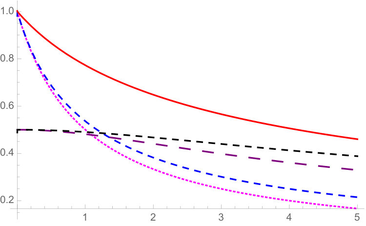 Figure 1
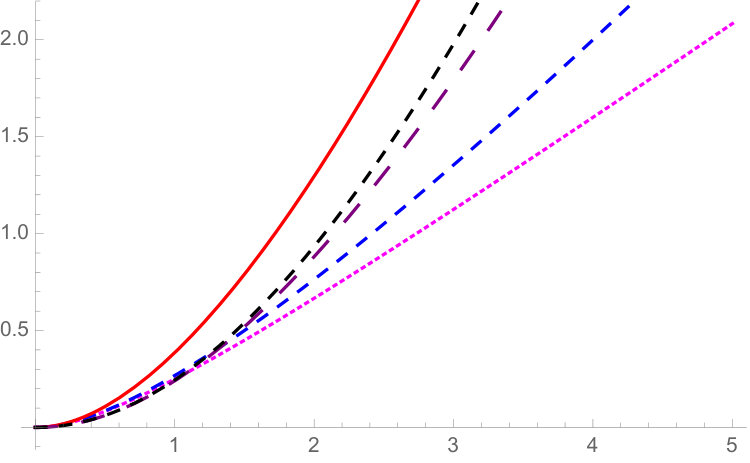 Figure 2
Peer Reviews
No public reviews on file for this paper yet. If you reviewed it on a platform where reviews are public (OpenReview, ICLR, NeurIPS, ICML), you can paste yours below so the community can read it here.
Videos
No videos yet. Explain this paper in a talk, walkthrough, or lecture? Add one.
Taxonomy
TopicsAdvanced Numerical Analysis Techniques · Mathematical Inequalities and Applications · Optimization and Variational Analysis
The Bennett-Orlicz norm
Jon A. Wellnerlabel=e1][email protected] [[ Department of Statistics
University of Washington
Seattle, WA 98195-4322
Abstract
Lederer and van de Geer (2013) introduced a new Orlicz norm, the Bernstein-Orlicz norm, which is connected to Bernstein type inequalities. Here we introduce another Orlicz norm, the Bennett-Orlicz norm, which is connected to Bennett type inequalities. The new Bennett-Orlicz norm yields inequalities for expectations of maxima which are potentially somewhat tighter than those resulting from the Bernstein-Orlicz norm when they are both applicable. We discuss cross connections between these norms, exponential inequalities of the Bernstein, Bennett, and Prokhorov types, and make comparisons with results of Talagrand (1989, 1994), and Boucheron, Lugosi, and Massart (2013).
60E15,
60F10,
Bennett’s inequality,
exponential bound,
Maximal inequality,
Orlicz norm,
Poisson,
Prokhorov’s inequality,
keywords:
[class=AMS]
keywords:
label=u1,url]http://www.stat.washington.edu/jaw/
t1Supported in part by NSF Grants DMS-1104832 and DMS 1566514, and NI-AID grant 2R01 AI291968-04
Contents
- 1 Orlicz norms and maximal inequalities
- 2 The Bernstein-Orlicz norm
- 3 Bennett’s inequality and the Bennett-Orlicz norm
- 4 Prokhorov’s “arcsinh” exponential bound and Orlicz norms
- 5 Comparisons with some results of Talagrand
- 6 Appendix 1: Lambert’s function ; inverses of and
- 7 Appendix 2: General versions of Lemmas 1-5
1 Orlicz norms and maximal inequalities
Let be an increasing convex function from onto . Such a function is called a Young-Orlicz modulus by Dudley [1999], and a Young modulus by de la Peña and Giné [1999]. Let be a random variable. The Orlicz norm is defined by
[TABLE]
where the infimum over the empty set is . By Jensen’s inequality it is easily shown that this does define a norm on the set of random variables for which is finite. The most important functions for a variety of applications are those of the form for , and in particular and corresponding to random variables which are “sub-exponential” or “sub-Gaussian” respectively. See Krasnosel*′skiĭ and Rutickiĭ [1961], Dudley [1999], Arcones and Giné [1995], de la Peña and Giné [1999], and van der Vaart and Wellner [1996] for further background on Orlicz norms, and see Rao and Ren [1991], Krasnosel′*skiĭ and Rutickiĭ [1961], and Hewitt and Stromberg [1975] for more information about Birnbaum-Orlicz spaces.
The following useful lemmas are from van der Vaart and Wellner [1996], pages 95-97, and Arcones and Giné [1995] (see also de la Peña and Giné [1999], pages 188-190), respectively.
Lemma 1.1**.**
Let be a convex, nondecreasing, nonzero function with and for some constant . Then, for any random variables ,
[TABLE]
*where is a constant depending only on .
Lemma 1.2**.**
Let be a Young Modulus satisfying
[TABLE]
Then for some constant depending only on and every sequence of random variables ,
[TABLE]
The inequality (1.1) shows that if Orlicz norms for individual random variables are under control, then the Orlicz norm of the maximum of the ’s is controlled by a constant times times the maximum of the individual Orlicz norms. The inequality (1.2) shows a stronger related Orlicz norm control of the supremum of an entire sequence divided by if the supremum of the individual Orlicz norms is finite. Lemma 1.2 implies Lemma 1.1 for Young functions of exponential type (such as with ), but it does not hold for power type Young functions such as , . These latter Young functions continue to be covered by Lemma 1.1. Arcones and Giné [1995] carefully define Young moduli for all and use Lemma 1.2 to establish laws of the iterated logarithm for U-statistics.
A general theme is that if and we have control of the individual Orlicz norms, then Lemma 1.1 or Lemma 1.2 applied with will yield a better bound than with in the sense that .
Here we are interested in functions of the form
[TABLE]
where is a nondecreasing convex function with not of the form . In fact, the particular functions of interest here are (scaled versions of):
[TABLE]
for the particular . The functions and are related to Bernstein exponential bounds and refinements thereof due to Birgé and Massart [1998], while the function is related to Bennett’s inequality (Bennett [1962]), and is related to Prokhorov’s inequality (Prokhorov [1959]).
van de Geer and Lederer [2013] studied the family of Orlicz norms defined in terms of scaled versions of , and called called them Bernstein-Orlicz norms. Our primary goal here is to compare and contrast the Orlicz norms defined in terms of , , , and . We begin in the next section by reviewing the Bernstein-Orlicz norm(s) as defined by van de Geer and Lederer [2013]. Section 3 gives corresponding results for what we call the Bennett-Orlicz norm(s) corresponding to the function . In Section 4 we give further comparisons and two applications.
2 The Bernstein-Orlicz norm
For a given number , van de Geer and Lederer [2013] have defined the Bernstein-Orlicz norm with
[TABLE]
It is easily seen that
[TABLE]
The following three lemmas of van de Geer and Lederer [2013] should be compared with the development on page 96 of van der Vaart and Wellner [1996].
Lemma 2.1**.**
Let . Then
[TABLE]
or, equivalently, with ,
[TABLE]
or
[TABLE]
Lemma 2.2**.**
Suppose that for some and we have
[TABLE]
Equivalently, the inequality (2.3) holds. Then .
Example 2.1**.**
Suppose that . Then it is well-known (see e.g. Boucheron et al. [2013], page 23), that
[TABLE]
where . Thus the inequality involving holds with and . Thus , . We conclude from Lemma 2.2 that
[TABLE]
Pisier [1983] and Pollard [1990] showed how to bound the Orlicz norm of the maximum of random variables with bounded Orlicz norms; see also de la Peña and Giné [1999], section 4.3, and van der Vaart and Wellner [1996], Lemma 2.2.2, page 96. The following bound for the expectation of the maximum was given by van de Geer and Lederer [2013]; also see Boucheron et al. [2013], Theorem 2.5, pages 32-33.
Lemma 2.3**.**
Let and be positive constants, and let be random variables satisfying . Then
[TABLE]
Corollary 2.1**.**
For
[TABLE]
In particular when for
[TABLE]
Proof. This follows from Lemma 2.3 since for . The Poisson special case then follows from Example 2.1.
It will be helpful to relate to several functions appearing frequently in the theory of exponential bounds as follows: for , we define
[TABLE]
It is easily shown (see e.g. Boucheron et al. [2013] Exercise 2.8, page 47) that
[TABLE]
A trivial restatement of the inequality on the left above and some algebra and easy inequalities yield
[TABLE]
The latter inequalities imply that the Orlicz norms based on and are equivalent up to constants.
One reason the functions and are so useful is that they both have explicit inverses: from Boucheron, Lugosi, and Massart (2013), page 29, for and direct calculation for ,
[TABLE]
To relate the inequalities in Lemmas 2.1 and 2.2 to more standard inequalities (with names) we note that
[TABLE]
This implies immediately that the inequality in Lemma 2.2 can be rewritten as
[TABLE]
Here is a formal statement of a proposition relating exponential tail bounds in the traditional Bernstein form in terms of to tail bounds in terms of the (larger) function .
Proposition 2.1**.**
Suppose that a random variable satisfies
[TABLE]
for numbers . Then the hypothesis of Lemma 2.2 holds with and given by and :
[TABLE]
Proof. This follows from (2.7) and elementary manipulations.
The classical route to proving inequalities of the form given in (2.8) for sums of independent random variables is via Bernstein’s inequality; see for example van der Vaart and Wellner [1996] Lemmas 2.2.9 and 2.2.11, pages 102 and 103, or Boucheron et al. [2013], Theorem 2.10, page 37. But the recent developments of concentration inequalities via Stein’s method yields inequalities of the form given in (2.8) for many random variables which are not sums of independent random variables: see, for example, Ghosh and Goldstein [2011a, b] and Goldstein and Işlak [2014]. The point of the previous proposition is that (up to constants) these inequalities in terms of can be re-expressed in terms of the (larger) function .
3 Bennett’s inequality and the Bennett-Orlicz norm
We begin with a statement of a version of Bennett’s inequality for sums of bounded random variables; see Bennett [1962], Shorack and Wellner [1986], and Boucheron et al. [2013]. Let and . This function arises in Bennett’s inequality for bounded random variables and elsewhere; see e.g. Bennett [1962], Shorack and Wellner [1986], and Boucheron et al. [2013], page 35 (but note that their is our ). As noted in Example 1 above, the function also appears in exponential bounds for Poisson random variables: see Shorack and Wellner [1986] page 485, and Boucheron et al. [2013] page 23.
Proposition 3.1**.**
(Bennett) (i) Let be independent with , , . Let , . Then with ,
[TABLE]
*for all .
(ii) If, in addition, , then*
[TABLE]
Using the inequality , it follows that
[TABLE]
Thus an inequality of the form of that in Lemma 2.1 holds with and . Thus and . It follows from Lemma 2.2 that
[TABLE]
or
[TABLE]
But this bound has not taken advantage of the fact the the first bound above involves the function (or ) rather than . It would seem to be of potential interest to develop an Orlicz norm based on the function rather than the function . Motivated by the first inequality in Proposition 3.1, we define for each a new Orlicz norm based on the function as follows.
[TABLE]
Since is convex, , and is increasing on , it follows that defines a valid Orlicz norm (as defined in Section 1) for each :
[TABLE]
We call the Bennett-Orlicz norm of . Note that with ,
[TABLE]
We first relate to and to the usual Gaussian Orlicz norm defined by .
Proposition 3.2**.**
(i) for all .
(ii) for .*
Proof. (i) follows since for all ; see Shorack and Wellner [1986], Proposition 11.1.1, page 441. To show that (ii) holds, note that by (2.1)
[TABLE]
Thus the claimed inequality in (ii) is equivalent to
[TABLE]
or equivalently
[TABLE]
But the inequality in the last display holds in view of (2.6).
Note that while and have explicit inverses given in terms of and by (2) and (2.4), inverses of the functions and can only be written in terms of Lambert’s function (also called the product log function) satisfying ; see Corless et al. [1996]. But this slight difficulty is easily overcome by way of several nice inequalities for . By use of and the inequalities developed in the Appendix, Section 6, we obtain the following proposition concerning .
Proposition 3.3**.**
(i) for .
(ii) Furthermore, with denoting the Lambert function,*
[TABLE]
(iii) If , then
[TABLE]
(iv) If , then
[TABLE]
(v) If , then
[TABLE]
(vi)
[TABLE]
Proof. (i) follows immediately from Proposition 3.2. (ii) follows from the definition of and direct computation for the first part; the second part follows from Lemma 6.1. The inequality in (iii) follows from (ii) and Lemma 6.2. The first inequality in (iv) follows from (iii) since for . The second inequality in (iv) follows by noting that
[TABLE]
if . (v) follows from (ii) and Lemma 6.3, part (iv).
Lemmas 2.1 and 2.2 by van de Geer and Lederer [2013] as stated in Section 2 should be compared with the development on page 96 of van der Vaart and Wellner [1996]. We now show that the following analogues of Lemmas 2.1 - 2.3 hold for .
Lemma 3.1**.**
Let . Then
[TABLE]
where and is the inverse of (so that ).
Proof. Let . Since implies , it follows that for any we have
[TABLE]
Lemma 3.2**.**
Suppose that for some we have
[TABLE]
Equivalently,
[TABLE]
Then .
Proof. Let . We compute
[TABLE]
Choosing this yields
[TABLE]
Hence we conclude that .
Corollary 3.1**.**
*(i) If , then .
(ii) If are i.i.d. Bernoulli, then*
[TABLE]
(iii) If , then for every . By taking the limit on and noting that as this yields . In this case it is known that . (See van der Vaart and Wellner [1996], Exercise 2.2.1, page 105.)
Now for an inequality paralleling Lemma 2.3 for the Bernstein-Orlicz norm:
Lemma 3.3**.**
Let and be constants, and let be random variables satisfying . Then
[TABLE]
Furthermore,
[TABLE]
for all such that (or ).
Remark 3.1**.**
The point of this last bound is that it gives an explicit trade-off between the Gaussian component (the term ) and the Poisson component (the term ) governed by a Bennett type inequality. In contrast, the bounds obtained by van de Geer and Lederer [2013] yield a trade-off between the Gaussian world and the sub-exponential world governed by a Bernstein type inequality.
Proof. We write . Let . Then by Jensen’s inequality
[TABLE]
Therefore,
[TABLE]
The remaining claims follow from Proposition 3.3.
Here are analogues of Lemmas 4 and 5 of van de Geer and Lederer [2013].
Lemma 3.4**.**
Let be random variables satisfying
[TABLE]
for some and . Then, for all
[TABLE]
Proof. For any and concavity of together with imply that
[TABLE]
Therefore, by using a union bound and Lemma 3.1
[TABLE]
Lemma 3.5**.**
Let be random variables satisfying (3.7). Then
[TABLE]
Proof. Let
[TABLE]
Then Lemma 3.4 implies that
[TABLE]
Then the conclusion follows from Lemma 3.2.
4 Prokhorov’s “arcsinh” exponential bound and Orlicz norms
Another important exponential bound for sums of independent bounded random variables is due to Prokhorov [1959]. As will be seen below, Prokhorov’s bound involves another function (rather than of Bennett’s inequality) given by
[TABLE]
Suppose that are independent random variables with and for some . Let , and set , . Prokhorov’s “arcsinh” exponential bound is as follows:
Proposition 4.1**.**
(Prokhorov) If the ’s satisfy the above assumptions, then
[TABLE]
Equivalently, with and ,
[TABLE]
See e.g. Prokhorov [1959], Stout [1974], de la Peña and Giné [1999], Johnson et al. [1985], and Kruglov [2006] . Johnson et al. [1985] use Prokhorov’s inequality to control Orlicz norms for functions of the form with and use the resulting inequalities to show that the optimal constants in Rosenthal’s inequalities grow as .
Kruglov [2006] gives an improvement of Prokhorov’s inequality which involves replacing by
[TABLE]
Note that Prokhorov’s inequality is of the same form as Bennett’s inequality (3.1) in Proposition 3.1, but with Bennett’s replaced by Prokhorov’s .
Thus we want to compare Prokhorov’s inequality (and Kruglov’s improvement thereof) to Bennett’s inequality. As can be seen from the above development, this boils down to comparison of the functions , , and . The following lemma makes a number of comparisons and contrasts between the functions , , and .
Lemma 4.1**.**
*(Comparison of , , and )
(i)(a) for all .
(i)(b) for all .
(ii)(a) for all .
(ii)(b) for all .
(ii)(c) for all .
(iii)(a) as ; as .
(iii)(b) as ; as .
(iii)(c) as ; as .
(iii)(d) as ; as .
(iii)(e) as ; as .*
(iv)(a) where
[TABLE]
(iv)(b) where
[TABLE]
(iv)(c) where
[TABLE]
Proof. (i) We first prove that . Let ; thus
[TABLE]
Then and
[TABLE]
also has . Note that and hence . Thus
[TABLE]
and hence
[TABLE]
and it suffices to show that the right side is for all . Thus we let
[TABLE]
Let . Then and we compute
[TABLE]
so that and the numerator, , is easily seen to be non-negative since implies for all . Thus .
Kruglov [2006] shows that . Now we show that . Note that with ,
[TABLE]
has and (as was shown above in (4.3) ). Thus .
(i)(b) The inequalities for the inverse functions follow immediately from the inequalities for the functions themselves in (i)(a).
(ii)(a) To show that the first inequality holds, consider
[TABLE]
Then and
[TABLE]
Thus and . The second inequality in (ii)(a) is trivial.
(ii)(b) This follows easily from for all .
(ii)(c) This follows from (i)(a) and (ii)(b).
(iii)(a) This follows from as ; see Proposition 11.1.1, page 441, Shorack and Wellner [1986].
(iii)(b) Now
[TABLE]
with , and
[TABLE]
with . Therefore
[TABLE]
and
[TABLE]
(iii)(c) Now
[TABLE]
where and is decreasing. Thus for some and we conclude that as .
(iv)(a) The first part is a restatement of (ii)(a). The second part follows from (2.7): , and the claim follows by definition of .
(iv)(b) The first inequality is a restatement of (ii)(b). The second inequality follows since where is decreasing, so
[TABLE]
To prove the third inequality, note that
[TABLE]
holds if , or if . Then rearrange and take for .
(iv)(c) The first inequality follows from (ii)(c). The second inequality follows by arguing as in (iv)(b), but now without the complicating second factor: note that
[TABLE]
since is decreasing.
Discussion: 1. Even though Kruglov’s inequality improves on Prokhorov’s inequality, (ia) of Lemma 4.1 shows that Bennett’s inequality dominates both Kruglov’s improvement of Prokhorov’s inequality and Prokhorov’s inequality itself: .
2. (ii) of Lemma 4.1 shows that all three of the inequalities, Bennett, Kruglov, and Prokhorov, are based on functions , , and which are bounded below by for all . On the other hand, (ii)(d) shows that both and are very nearly equivalent for large , but that although grows at the same rate as and , is smaller by a multiplicative factor of as .
3. (iii)(a-c) of Lemma 4.1 shows that as while for both and ; thus is larger at by a factor of . Furthermore, the difference is of order as , while the difference is only of order as .
4. (iv) of Lemma 4.1 re-expresses the behavior of the Kruglov and Prokhorov inequalities for small values of in terms of the corresponding functions.
The upshot of all of these comparisons is that Bennett’s inequality dominates both the Kruglov and Prokhorov inequalities. Figures 1 - 2 give graphical versions of these comparisons as well as comparisons to the Bernstein type functions and .
5 Comparisons with some results of Talagrand
Our goal in this section is to give comparisons with some results of Talagrand [1989] and Talagrand [1994], especially his Theorem 3.5, page 45, and Proposition 6.5, page 58.
Talagrand [1994] defines a function as follows:
[TABLE]
Because of the square-root on the log term, this can be regarded as corresponding to a “sub - Bennett” type exponential bound. One of the interesting properties of established by Talagrand [1994] is given in the following lemma:
Lemma 5.1**.**
There is a number depending on only such that
[TABLE]
This is Lemma 3.6 of Talagrand [1994] page 47. Talagrand uses this Lemma to develop a Kiefer-type inequality: see also van der Vaart and Wellner [1996], Corollary A.6.3. In the basic Kiefer type inequality for Binomial random variables, van der Vaart and Wellner [1996], Corollary A.6.3, it follows that
[TABLE]
for ; i.e. for .
A similar fact holds for any exponential bound of the Bennett type under a certain boundedness hypothesis. Suppose that
[TABLE]
and that for all . Then, since is decreasing, for
[TABLE]
where the term can be made arbitrarily large by choosing sufficiently small. Here the second inequality follows from the fact that
[TABLE]
Proof of (5.2): Since where , we can write, with ,
[TABLE]
where both terms are clearly non-negative.
Now we consider another basic inequality due to Talagrand [1994]. Suppose that
[TABLE]
satisfies the following three properties:
(a) implies that for .
(b) .
(c) .
Then if are i.i.d. non-atomic on and , for some universal constant we have, for ,
[TABLE]
As noted by Talagrand [1994], this follows from an isoperimetric inequality established in Talagrand [1989], but it is also a consequence of results of Talagrand [1991, 1995]. Here we simply note that it can be rephrased as a Bennett type inequality: for all
[TABLE]
This follows by simply checking that
[TABLE]
for .
Also see Ledoux [2001], Theorem 7.5, page 142 and Corollary 7.8, page 148; Massart [2000], and Boucheron et al. [2013], Theorem 6.12, page 182.
One further remark seems to be in order: Talagrand [1989] Theorem 2 and Proposition 12, shows that Orlicz norms of the Bennett type are “too large” to yield nice generalizations of the classical Hoffmann-Jørgensen inequality in the setting of sums of independent bounded sequences in a general Banach space. This follows by noting that Talagrand’s condition (2.11) fails for the Bennett-Orlicz norm as defined in (3.2).
6 Appendix 1: Lambert’s function ; inverses of and
Let and for . The function is convex, decreasing on , increasing on , with ; see Shorack and Wellner [1986], page 439. The Lambert, or product log function, (see e.g. Corless et al. [1996] and satisfies for . As noted by Boucheron et al. [2013], problem 2.18, the inverse functions (for the function ) and (for the function ) can be expressed in terms of the function . Here are some facts about :
Fact 1: is multi-valued on with two branches and
where , , and .
Fact 2: is monotone increasing on with and .
See Roy and Olver [2010], section 4.13, page 111; and Corless et al. [1996].
In the following we simply write for . The following lemma shows that the inverses of the functions and can be expressed in terms of .
Lemma 6.1**.**
*( and inverses in terms of )
(i) For *
[TABLE]
(ii) For
[TABLE]
Proof. If is as in the display we have, since ,
[TABLE]
Thus (6.1) holds. Then (6.2) follows immediately.
In view of Lemma 6.1, the following lower bounds on the function will be useful in deriving upper bounds on and .
Lemma 6.2**.**
(A lower bound for ) For
[TABLE]
Proof. We first prove (6.3) for . Since is increasing for , the claimed inequality is equivalent to
[TABLE]
for where . But then the last display is equivalent to
[TABLE]
or
[TABLE]
Now , , and has , , and for with , we find that . Thus the claimed bound holds for . For the bound holds trivially since while .
Combining Lemma 6.1 with the lower bounds for given in Lemma 6.2 yields the following upper bounds for and . The second and third parts of the following lemma are motivated by the fact that where as ; see Shorack and Wellner [1986], Proposition 4.4.1, page 441.
Lemma 6.3**.**
*(Upper bounds for and )
(i) For *
[TABLE]
(ii) For ,
[TABLE]
(iii) For with ,
[TABLE]
*In particular, with , the bound holds for , and with , the bound holds for .
(iv) For ,*
[TABLE]
Proof. (i) Follows from (i) of Lemma 6.1 together with Lemma 6.2. Note that and is increasing for .
(ii) follows from (ii) of Lemma 6.1 and Lemma 6.2.
(iii) To show that (6.6) holds, note that the inequality is equivalent to , and hence, by taking , to the inequality
[TABLE]
where by Lemma 4.1 (iva) (or by (10) of Proposition 11.4.1, Shorack and Wellner [1986] page 441). But then we have
[TABLE]
where the last inequality holds if . Hence the inequality in (iii) holds for . Finally, (iv) holds by combining the bounds in (ii) and (iii).
7 Appendix 2: General versions of Lemmas 1-5
Now consider Young functions of the form where is assumed to be convex and nondecreasing with . (Note that we have changed notation in this section: the functions and for in Sections 1 - 6 are denoted here by .) Our goal in this section is to give general versions of Lemmas 1 - 5 of van de Geer and Lederer [2013] and section 3 above. The advantage of this formulation is that the resulting lemmas apply to all the special cases treated in Sections 2 and 3 and more.
Lemma 7.1**.**
Suppose that . Then for all
[TABLE]
For the general version of Lemma 2 we consider a scaled version of as follows:
[TABLE]
Lemma 7.2**.**
Suppose that for some and
[TABLE]
Then .
Lemma 7.3**.**
Suppose that is non-decreasing, convex, with . Suppose that are random variables with . Then
[TABLE]
Lemma 7.4**.**
Suppose that is non-decreasing, convex, with . Suppose that are random variables with . Then
[TABLE]
Lemma 7.5**.**
Suppose that is non-decreasing, convex, with . Suppose that are random variables with . Then
[TABLE]
Proof of Lemma 7.1. For all
[TABLE]
Thus letting yields
[TABLE]
Proof of Lemma 7.2. Let . We compute
[TABLE]
by choosing .
Proof of Lemma 7.3. Let . Then by Jensen’s inequality and convexity of
[TABLE]
Letting yields
[TABLE]
Proof of Lemma 7.4. For any and concavity of implies that
[TABLE]
Therefore, by using this with and , a union bound, and Lemma 7.1,
[TABLE]
Proof of Lemma 7.5. By Lemma 7.4
[TABLE]
so the hypothesis of Lemma 7.2 holds for
[TABLE]
with and replaced by . Thus the conclusion of Lemma 7.2 holds for with these choices of and : .
**Acknowledgement: ** I owe thanks to Evan Greene and Johannes Lederer for several helpful conversations and suggestions. Thanks are also due to Richard Nickl for a query concerning Prokhorov’s inequality.
The reference list from the paper itself. Each links out to its DOI / PubMed record.
- 1Arcones and Giné [1995] Arcones, M. A. and Giné, E. (1995). On the law of the iterated logarithm for canonical U 𝑈 U -statistics and processes. Stochastic Process. Appl. , 58 (2), 217–245.
- 2Bennett [1962] Bennett, G. (1962). Probability inequalities for the sum of independent random variables. Journal of the American Statistical Association , 57 , 33–45.
- 3Birgé and Massart [1998] Birgé, L. and Massart, P. (1998). Minimum contrast estimators on sieves: exponential bounds and rates of convergence. Bernoulli , 4 (3), 329–375.
- 4Boucheron et al. [2013] Boucheron, S., Lugosi, G., and Massart, P. (2013). Concentration Inequalities . Oxford University Press, Oxford.
- 5Corless et al. [1996] Corless, R. M., Gonnet, G. H., Hare, D. E. G., Jeffrey, D. J., and Knuth, D. E. (1996). On the Lambert W 𝑊 W function. Adv. Comput. Math. , 5 (4), 329–359.
- 6de la Peña and Giné [1999] de la Peña, V. H. and Giné, E. (1999). Decoupling; From dependence to independence . Probability and its Applications (New York). Springer-Verlag, New York.
- 7Dudley [1999] Dudley, R. M. (1999). Uniform Central Limit Theorems , volume 63 of Cambridge Studies in Advanced Mathematics . Cambridge University Press, Cambridge.
- 8Ghosh and Goldstein [2011 a] Ghosh, S. and Goldstein, L. (2011 a). Applications of size biased couplings for concentration of measures. Electron. Commun. Probab. , 16 , 70–83.