Sum-set Inequalities from Aligned Image Sets: Instruments for Robust GDoF Bounds
Arash Gholami Davoodi, Syed A. Jafar

TL;DR
This paper introduces new sum-set inequalities derived from aligned image sets, providing robust tools for deriving GDoF bounds in complex wireless networks with multiple antennas and uncertain channel conditions.
Contribution
It generalizes the aligned image sets approach to create sum-set inequalities that aid in GDoF analysis for multi-antenna wireless networks with channel uncertainty.
Findings
Derived tight GDoF bounds for a two-user interference channel with multiple antennas.
Generalized sum-set inequalities applicable to various wireless network configurations.
Provided a new information-theoretic framework for analyzing channel uncertainty effects.
Abstract
We present sum-set inequalities specialized to the generalized degrees of freedom (GDoF) framework. These are information theoretic lower bounds on the entropy of bounded density linear combinations of discrete, power-limited dependent random variables in terms of the joint entropies of arbitrary linear combinations of new random variables that are obtained by power level partitioning of the original random variables. These bounds generalize the aligned image sets approach, and are useful instruments to obtain GDoF characterizations for wireless networks, especially with multiple antenna nodes, subject to arbitrary channel strength and channel uncertainty levels. To demonstrate the utility of these bounds, we consider a non-trivial instance of wireless networks - a two user interference channel with different number of antennas at each node, and different levels of partial channel…
Click any figure to enlarge with its caption.
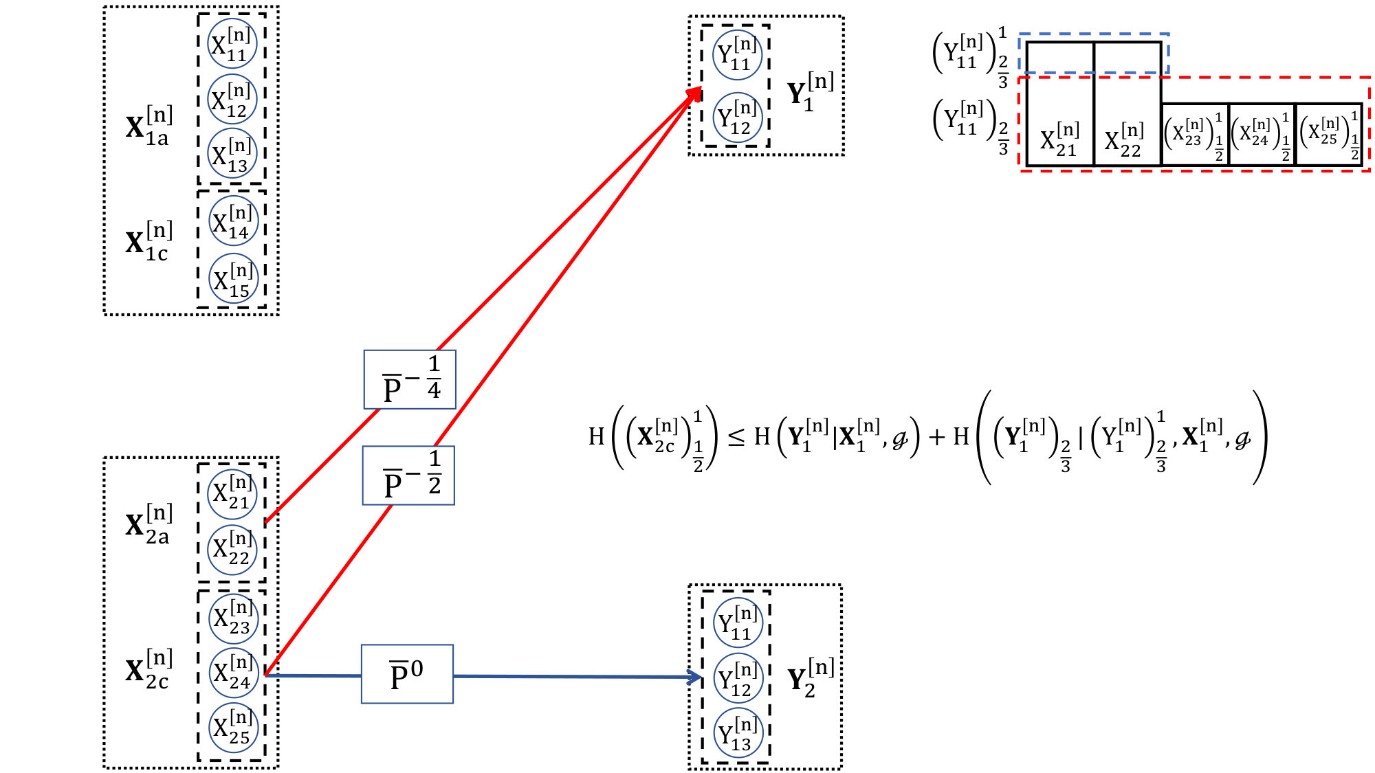 Figure 1
Peer Reviews
No public reviews on file for this paper yet. If you reviewed it on a platform where reviews are public (OpenReview, ICLR, NeurIPS, ICML), you can paste yours below so the community can read it here.
Videos
No videos yet. Explain this paper in a talk, walkthrough, or lecture? Add one.
Sum-set Inequalities from Aligned Image Sets:
Instruments for Robust GDoF Bounds
Arash Gholami Davoodi and Syed A. Jafar
Center for Pervasive Communications and Computing (CPCC)
University of California Irvine, Irvine, CA 92697
Email: {gholamid, syed}@uci.edu
Abstract
We present sum-set inequalities specialized to the generalized degrees of freedom (GDoF) framework. These are information theoretic lower bounds on the entropy of bounded density linear combinations of discrete, power-limited dependent random variables in terms of the joint entropies of arbitrary linear combinations of new random variables that are obtained by power level partitioning of the original random variables. These bounds generalize the aligned image sets approach, and are useful instruments to obtain GDoF characterizations for wireless networks, especially with multiple antenna nodes, subject to arbitrary channel strength and channel uncertainty levels. To demonstrate the utility of these bounds, we consider a non-trivial instance of wireless networks – a two user interference channel with different number of antennas at each node, and different levels of partial channel knowledge available to the transmitters. We obtain tight GDoF characterization for specific instance of this channel with the aid of sum-set inequalities.
1 Introduction
Originating in additive combinatorics, sum-set inequalities are bounds on the cardinalities of sum-sets (given , the sumset ). Crossing over to network information theory, sum-set inequalities represent bounds on the entropies of sums of random variables, typically expressed in terms of the entropies of the constituent random variables. Prominent examples of such inequalities include Ruzsa’s sum-triangle inequality in additive combinatorics [1] and the entropy power inequality in information theory [2]. Sum-set inequalities are essential to the study of the capacity of wireless interference networks. This is particularly true for the studies of capacity approximations known as generalized degrees of freedom (GDoF) [3] through deterministic models [4] which de-emphasize the additive noise to place the focus exclusively on the interactions between signals. Received signals in wireless networks are comprised of sums (more generally, linear combinations) of codewords from various codebooks, sent from various transmitters. GDoF optimal schemes seek to maximize the entropy of received linear combinations of signals where they are desired, while simultaneously minimizing the entropy of received linear combinations of the same signals where they are undesired (e.g., by zero-forcing or interference alignment [5]). The fundamental constraints on the structure of sum-sets, as revealed by sum-set inequalities are therefore the critical determinants of the GDoF of wireless interference networks. However, in spite of much recent progress in translating sum-set inequalities from additive combinatorics to network information theory [6], the structure of sum sets remains scarcely understood, and continues to be an impediment for GDoF characterizations. In fact, the intricacies of the sum-set structure are such that even a coarse metric like the degrees of freedom (DoF) for constant channel realizations turns out to be sensitive to fragile details of no conceivable practical relevance – e.g., whether the channel coefficients take rational or irrational values [7].
Useful insights need robust models and metrics which respond predominantly to those parameters that are known to be of the greatest practical significance. For wireless interference networks, the most significant aspects include the interplay of spatial dimensions (especially if multiple antennas are involved) with channel strengths and channel uncertainty levels [8]. Fortunately, the GDoF framework incorporates all three – spatial dimensions, channel uncertainties and channel strength levels. Furthermore, the fragile aspects of the GDoF metric may be avoided by restricting channel state information at the transmitters (CSIT) to finite precision.
The study of DoF under finite precision channel knowledge was initiated by Lapidoth et al. in [9], leading to a conjecture on the collapse of DoF. In spite of various attempts at proving or disproving the conjecture the conjecture remained open for a decade. It was ultimately settled using an approach based on a combinatorial accounting of the size of the aligned image sets (AIS) under finite precision channel knowledge, in short the AIS approach in [10]. The AIS approach modeled finite precision channel knowledge as the assumption that from the transmitters’ perspective, all joint and conditional probability density functions of channel coefficients exist and are bounded. The bounded density assumption was found to be compatible with various levels of channel strengths and channel knowledge. The AIS approach was further developed to fully characterize the GDoF of the user MISO BC (broadcast channel with two antennas at the transmitter and one antenna at each of the two receivers) for arbitrary channel strength levels and arbitrary channel uncertainty levels for each channel coefficient, establishing the GDoF optimality of robust schemes in all cases [11]. It has also led to GDoF characterizations for the user symmetric IC under finite precision CSIT [12], symmetric instances of user MISO BC [13], symmetric DoF of interference networks with finite precision CSIT and perfect CSIR [14], and GDoF of user symmetric MIMO IC with partial CSIT [15]. Indeed, there exists the distant but exciting possibility that the AIS approach may ultimately lead us to the GDoF characterizations of broad classes of wireless networks. If so, then the resulting comprehensive and fundamental understanding of these complex networks – the interplay between spatial dimensions, channel strengths, and channel uncertainty levels – would be invaluable. However, in order to get there, it is evident that a robust understanding of sum-sets will be needed. Specifically, there is the need to identify the key sum-set inequalities for signals subject to arbitrary power levels under the robust bounded density assumption. This is the goal that we pursue in this work.
The paper is organized as follows. Section provides the necessary definitions. The main results, i.e., the sum-set inequalities are presented in Section 3 through progressively generalized theorems for ease of exposition, starting from a single-letter single-antenna form to the general multi-letter multi-antenna form that is needed to derive GDoF outer bounds for MIMO networks. In Section 4, we present an example to show how these sum-set inequalities allow us to obtain new GDoF characterizations for non-trivial networks under partial CSIT111Channel uncertainty and channel strengths are interchangeable to a certain extent in MIMO interference networks, because the channel uncertainty level governs the strength of residual interference when signals are zero-forced. This is previously noted in [16]. that were previously open. The example is comprised of a user MIMO interference channel (IC) where the two transmitters are equipped with and antennas, their corresponding receivers with and antennas, the channel strength parameters are chosen to be and partial CSIT parameters are chosen to be and . Remarkably, building upon these insights, in [17] we have found that the sum-set inequalities allow us to fully characterize the GDoF region of the MIMO IC with arbitrary antenna configurations under arbitrary levels of partial CSIT. Moreover, sum-set inequalities allowed the authors to characterize the full GDoF region of the two user MIMO BC with arbitrary antenna configurations under arbitrary levels of partial CSIT in [18].
Notation: For , define the notation . The cardinality of a set is denoted as . The notation stands for . Moreover, also stands for . The support of a random variable is denoted as supp. The sets and stand for the set of real numbers and the set of all -tuples of real numbers respectively. Moreover, the set is defined as the set of all pairs of non-negative numbers. If is a set of random variables, then refers to the joint entropy of the random variables in . Conditional entropies, mutual information and joint and conditional probability densities of sets of random variables are similarly interpreted. Moreover, we use the Landau and notations as follows. For functions from to , denotes that . denotes that . We use to denote the probability function . For any real number we define as the largest integer that is smaller than or equal to when , the smallest integer that is larger than or equal to when , and itself when is an integer. We also define as maximum of the number and [math], i.e., . The number may be represented as if there is no cause for ambiguity.
2 Definitions
The information theoretic sum-set inequalities that we seek are motivated by the GDoF framework. Since in the next section we present general statements of sum-set inequalities, here we only present definitions needed for Section 3. The definitions needed for the MIMO IC setting that we use as an example, are presented in Section 4.
Definition 1** (Power Levels)**
Consider integer valued variables over alphabet ,
[TABLE]
where is a compact notation for . We refer to as power, and are primarily interested in limits as . Quantities that do not depend on will be referred to as constants. The constant denotes the power level of .
We are interested in sum-set inequalities in terms of entropies of random variables such as , normalized by as , while the power levels are held fixed. All the sumset inequalities in this work hold in this asymptotic sense, i.e., while disregarding terms that are negligible relative to . Such terms are denoted as terms.
Definition 2
For any nonnegative real numbers , and , define and as,
[TABLE]
In words, for any , retrieves the top power levels of , while retrieves the bottom levels of . retrieves only the part of that lies between power levels and . Note that can be expressed as for . Equivalently, suppose , , and . Then , . A conceptual illustration of power level partitions is shown in Figure 1.
Definition 3
For the vector , we define and as,
[TABLE]
Definition 4** (Bounded Density Channel Coefficients)**
Bounded density channels are represented by a set of real valued random variables, such that the magnitude of each random variable is bounded away from zero and infinity, , for some constants , and there exists a finite positive constant , such that for all finite cardinality disjoint subsets of , the joint probability density function of all random variables in , conditioned on all random variables in , exists and is bounded above by .
Definition 5** (Arbitrary Channel Coefficients)**
Let be a set of arbitrary constant values that are bounded above by , i.e., if then .
Definition 6
For real numbers and the vectors and define the notations , , and to represent,
[TABLE]
for distinct random variables , some arbitrary real valued and finite constants and some arbitrary non-negative real valued constants . For the vector we also define the notations and to represent,
[TABLE]
for distinct random variables and .
Note that, the subscript is used to distinguish among multiple linear combinations, and may be dropped if there is no potential for ambiguity. We refer to the functions as bounded density linear combinations.
Definition 7
For the linear combinations and where we define and as,
[TABLE]
Note that the terminology from Definition (6) is invoked in Definition (7). Figure 2 provides a visual illustration of and . From the definition of and in (12), it follows that,
[TABLE]
This is because all elements of are bounded from above by .
Definition 8
For any vector and non-negative integer numbers and less than , define
[TABLE]
Moreover, for the two vectors and define as .
3 Results
Theorem 1
For , consider random variables , all independent of , and define
[TABLE]
then
[TABLE]
The following remarks place Theorem 1 in perspective and discuss some of its generalizations.
Let denote the set of all bounded density channel coefficients that appear in , and let be a random variable such that conditioned on any , the channel coefficients satisfy the bounded density assumption. Then (22) generalizes to the following conditional form.
[TABLE]
The proof presented in Appendix A.1 covers this generalization. In various applications of these sum-set inequalities, the conditioning variable could represent terms such as , or . 2. 2.
A typical restriction in information theoretic sum-set inequalities is the independence of random variables. In contrast, note that the statement of Theorem 1 also holds for dependent random variables. 3. 3.
Since the linear combining coefficients involved in and can take arbitrary (including zero) values, several specializations of Theorem 1 follow immediately, e.g.,
[TABLE]
Figure 3 visually illustrates these inequalities in terms of the power levels.
Theorem 1 also holds if are replaced with bounded density linear combinations, i.e., . 5. 5.
While in the GDoF framework, Theorem 1 is typically used when as assumed, it is possible to generalize the result of Theorem 1 to allow . In that case, the inequality (22) becomes . The proof presented in Appendix A.1 covers this generalization. 6. 6.
The result of Theorem 1 lends itself to extensive generalizations in terms of the number of random variables, and the number of power level partitions. Such a generalization is presented in the following theorem.
Theorem 2
Consider non-negative numbers and random variables , independent of , and define
[TABLE]
* such that , , where we define*
[TABLE]
If for each ,
[TABLE]
then,
[TABLE]
Recall that for any real number , we define .
Theorem 1 is recovered as a special case of Theorem 2 if , , , and for any . 8. 8.
While applying Theorem 2 in the GDoF framework, a multi-letter extension is required. Such a generalization is presented in the following theorem. The same applies for extensions to complex valued random variables which can be obtained along the same lines as previous bounds based on the AIS approach, e.g., Section VII in [10].
Theorem 3
Consider non-negative numbers and random variables , , independent of , and define
[TABLE]
The channel uses are indexed by t$$\in\mathbb{N}. are subsets of such that whenever and , then
[TABLE]
if for each ,
[TABLE]
Note that, for any the set indicates what power levels are used by each . For instance enforces to be a linear combination of bottom part of for all , i.e., . 9. 9.
While applying Theorem 3 in the GDoF framework, a multi-antenna extension is required. The results of Theorem 3 can be generalized as follows,
Theorem 4
Consider non-negative numbers and random variables , , , independent of , and , define
[TABLE]
The channel uses are indexed by . such that , where
[TABLE]
If for all and for each ,
[TABLE]
then
[TABLE]
See Appendix A.2 for the proof of Theorem 4. Note that the proof of Theorem 4 also proves Theorem 2 and Theorem 3 which may be recovered as specializations of Theorem 4.
A visual illustration of an application of Theorem 4 is provided in Figure 5. 10. 10.
The results of Theorem 1 and its generalization in Theorem 4 can be further combined with sub-modularity properties of the entropy function222If is a finite set, a submodular function is a set function , where denotes the power set of , which satisfies the following property;
For every we have that [19]. to obtain a variety of sum-set inequalities specialized for different GDoF settings. 11. 11.
To show how the new sum-set inequalities presented in Theorem 4 are useful to obtain tight GDoF bounds in conjunction with submodularity properties of entropy, an example that arise in the context of the user MIMO IC is presented in Section 4.
4 GDoF Outer Bound for a User MIMO IC under Partial CSIT
In this section, as an example of the use of the sum-set inequalities, we obtain a tight GDoF outer bound for a non-trivial two user MIMO IC setting with asymmetric antenna configuration and asymmetric partial CSIT. Specifically, we consider the two user MIMO IC with as shown in Figure 6. We assume, and and derive a tight GDoF bound for this channel using our sum-set inequalities. Achievability for this case is already known from [17] and [20].
4.1 The Channel
The channel model for the two user MIMO IC with is defined by the following input-output equations.
[TABLE]
Here, and are the signal vectors sent from the first and second transmitters respectively, normalized so that each is subject to unit power constraint. and are the and received signal vectors at the first and second receivers, respectively. and are the and vectors whose components are zero-mean unit-variance additive white Gaussian noise (AWGN). The matrix is the channel fading coefficient matrix between the -th receiver and the -th transmitter for any . The entry in the -th row and -th column of the matrix is .
4.1.1 Partial CSIT
Under partial CSIT, the channel coefficients are represented as
[TABLE]
Recall that is the channel fading coefficient between the -th antenna of the -th receiver and the -th antenna of the -th transmitter. is the channel estimate and is the estimation error term. To avoid degenerate conditions, for each channel matrix , we require that all its submatrices are non-singular, i.e., their determinants are bound away from zero. To this end, for all , and for all choices of transmit antenna indices define the determinant as
[TABLE]
Then we require that there exists a positive constant , such that , for all The channel variables are distinct random variables drawn from the set . The realizations of are known to the transmitter, but the realizations of are not available to the transmitter. We also assume that the channel coefficients are bounded away from zero, i.e.,
[TABLE]
Note that under the partial CSIT model, the variance of the channel coefficients behaves as and the peak of the probability density function behaves as .
For any , in order to span the full range of partial channel knowledge at the transmitters, the corresponding range of parameters, assumed throughout this work, is . and correspond to the two extremes where the CSIT is essentially absent, or perfect, respectively. Note that the value of and will not affect the GDoF.
4.1.2 GDoF
The definitions of achievable rates and capacity region are standard. The DoF region is defined as
[TABLE]
4.2 Channel Model
The channel model is derived similar to the channel model for the general two user IC with arbitrary number of antennas in [12]. We will avoid repetition of explanations for those steps that are essentially identical to [12], and focus instead on the deviations from the original proof. As in [12], the starting point is to bound the problem with deterministic model, such that a GDoF outer bound on the deterministic model is also a GDoF outer bound for the original problem. Since the derivation of the deterministic model is essentially identical to [12], here we simply state the resulting equivalent deterministic model.
4.2.1 Equivalent Deterministic Model
As in [12], without loss of generality for DoF characterizations, we will use the deterministic model for the equivalent channel.
[TABLE]
for all . , , , , and are defined as,
[TABLE]
and , .
4.3 GDoF region of the two user MIMO IC
Theorem 5
The GDoF region of the two user MIMO IC with and , is as follows
[TABLE]
Note that, these bounds turns out to be tight, i.e., the achievability and the outer bounds coincide with each others, see [17].
Proof of Theorem 5 is relegated to Appendix A.3 and is straightforward except for the following lemma which is the main novelty of the outer bound proof. It is in deriving this key lemma that we require both the sum-set inequalities of Theorem 4 and the sub-modularity of entropy functions.
Lemma 1
For the two user MIMO IC with and levels of partial CSIT, we have,
[TABLE]
See Figure 7 for the comparison of the two sides of (58).
See Appendix B for proof of Lemma 1.
5 Conclusion
We present a class of sum-set inequalities for bounded set linear combinations of random variables typically encountered in the GDoF framework. The bounds are obtained by building upon the aligned image sets (AIS) approach. Through an example, we showed that these inequalities are useful for obtaining tight GDoF bounds for MIMO interference networks with arbitrary antenna configurations and arbitrary levels of channel uncertainty for each channel. Indeed, we expect these inequalities to be broadly useful for obtaining tight GDoF bounds for MIMO wireless interference and broadcast networks under varying levels of channel strengths and channel uncertainty.
Appendix A Proof of Theorems 1, 2, 3, 4 and 5
A.1 Proof of Theorem 1
A.1.1 Sketch of the proof
Let us start with a summary of the Aligned Image Sets approach that we use in this proof. We are only interested in maximum of difference of entropies of and conditioned on , i.e., . Following directly along the AIS approach [10], from the functional dependence argument it follows that without loss of generality can be assumed to be a function of . So, it follows that,
[TABLE]
where follows from chain rule and is true as is a function of . Thus, the difference of entropies is equal to . Now, for a given and channel realization , define aligned image set as the set of all which result in the same . In the other words, since is a function of , we define the set as the set of all values of which produce the same value for , as is produced by . Since uniform distribution maximizes the entropy,
[TABLE]
where is support of the random variable . (64) comes from the Jensen’s Inequality. Thus, the difference of the entropies is bounded by the log of expected value of cardinality of the aligned image set. Now, the most crucial step is to bound the cardinality of where we need to use Bounded Density Assumption of to bound the cardinality of . So, from the equation (64), \mbox{E}_{\mathcal{G}}\{|S_{\nu}(W,\mathcal{G})|\mid{\color[rgb]{0,0,1}\definecolor[named]{pgfstrokecolor}{rgb}{0,0,1}W=w}\} is what needed to be calculated. Expected value of size of the cardinality of aligned image set is equal to the summation of probability of alignment over all , or in the other words,
[TABLE]
where is defined as the probability that and correspond to the same . In the proof, we prove that \mbox{E}_{\mathcal{G}}\{|S_{\nu}(W,\mathcal{G})|\mid{\color[rgb]{0,0,1}\definecolor[named]{pgfstrokecolor}{rgb}{0,0,1}W=w}\} is bounded by from above for constants and . So, from the inequality (64), we have,
[TABLE]
for some constant if . As , (22) is concluded. The detailed arguments are presented next.
A.1.2 Functional Dependence
We start by showing that there is no loss of generality in the assumption that is a function of and , and therefore is a function of . Recall that is independent of . However, there may be multiple values of that cast the same image in . So the mapping from to is in general random. Let us denote it by i.e.
[TABLE]
In general, because the mapping may be random, is a random variable. Conditioning cannot increase entropy, therefore,
[TABLE]
Let be the mapping that minimizes the entropy term. Fix this as the deterministic mapping,
[TABLE]
so that now is a function of , and since is a function of , is equivalently a function of . Based on convenience, we may indicate the functional dependence in any of these forms as
[TABLE]
We note that the choice of mapping does not affect the positive entropy term but it minimizes .
A.1.3 Definition of Aligned Image Sets
The aligned image set containing the codeword for a given and realization is defined as the set of all values of that produces the same value as is produced by . Mathematically,
[TABLE]
Since we will need the average (over ) of the cardinality of an aligned image set, E, it is worthwhile to point out that the cardinality as a function of , is a bounded simple function, and therefore measurable.333A simple function is a finite sum of indicator functions of measurable sets [21]. It is bounded because its values are restricted to the set of natural numbers not greater than , where depends on coefficients of linear combinations and . Following the same steps as [10] it is a simple function too.
A.1.4 Bounding the Probability of Image Alignment
From (65), we have . Given , consider two distinct realizations of , say , and , which are produced by two distinct realizations of , denoted as and . For , define , , and as , , , and respectively.
[TABLE]
We wish to bound the probability that the images of these two codewords align, or in other words ,
[TABLE]
defining as we have
[TABLE]
So for fixed values of the random variable must take values within an interval of length no more than . If , then must take values in an interval of length no more than , the probability of which is no more than . Note that the integral of any real-valued measurable function over any measurable set can be bounded above by times the measure of the set , which for the interval reduces to the length of the interval [21]. Similarly, for fixed values of probability of alignment will be bounded by . As , and are two distinct realizations of , at least one of for is nonzero. So, it can be concluded that the probability is no more than where is defined as follows.
[TABLE]
A.1.5 Bounding the Average Size of Aligned Image Sets
From (65) we have to compute the following summation,
[TABLE]
Note that, from (73), and (74) the terms , and can be bounded from above by , and , respectively as and are less than for all and, and are also less than , respectively. Using the definition of Aligned Image Sets from A.1.3, we have,
[TABLE]
where the sets , and are defined as , and , respectively. For simplicity we defined as the constant . Now, let us bound each term in (80) separately. Note that our ultimate goal is to prove for some constants and , which along with (64) leads to the conclusion (22) when .
Let us compute the first summation in (80).
[TABLE]
(81) follows by bounding the terms from below by if . (1) is breaking the summation into multiplication of two summations, and (LABEL:poi11) is true because is bounded by one, so the summation of such terms can be at most . Finally, (1) follows by bounding from (73) and (74) as,
[TABLE]
where is a random variable which takes values in the interval . (85) is true as the partial sum of harmonic series can be bounded above by logarithmic function, i.e., . 2. 2.
The second term in (80), i.e., is bounded similarly by the exact term in equation (85) as the inequalities (81)-(85) remain true whether the summation is over or . 3. 3.
Finally, the third term in (80) is bounded from above by splitting the summation into four summations where in each summation the terms and are fixed to either zero or one. First of all let us write from , and as,
[TABLE]
where is a random variable depending on which takes values in the interval .
[TABLE]
where the function is defined as if and if . The numbers , , , , and are also defined as , , , , , and . The set is defined as the set of integer numbers . (LABEL:ppjj) is derived by replacing in . (90) follows as,
[TABLE]
where is true as the . (93) is derived by replacing from (88), (93) follows by breaking summation into two summations, and, (93) is true as minimum of any two numbers can be bounded above by one of them. Note that the first summation in (93) can be at most as is true only if . Moreover, can be true for at most integer numbers of . So, the first summation is at most 11. Second summation in (93) is bounded as,
[TABLE]
where (97) is concluded from the following two points,
- (a)
Each summand in the left summation (97) is reciprocal of a positive integer number, and reciprocal of any positive integer number, i.e., can be repeated in the left summation at most times as can have at most solutions in the set of for any fixed integer number .
[TABLE]
(99), (100) can be true only for integers of in the set of for any fixed integer number of . So, any reciprocal of any positive integer number, i.e., can be repeated at most 18 times in the left summation. 2. (b)
can only get integer numbers from the set , as is bounded from above by .
Finally, (95) is true as the partial sum of harmonic series can be bounded above by logarithmic function.
A.1.6 Combining the Bounds to Complete the Proof
Now, from (80), (85), and (95) since constant terms and are , we have,
[TABLE]
as (101) is true for all , from (65) we have,
[TABLE]
Note that, (22) is concluded when .
A.2 Proof of Theorem 2, 3 and 4
In this section we only present proof of Theorem 4 as Theorem 2 and 3 are obtained as special cases of Theorem 4.
Recall that,
[TABLE]
The channel uses are indexed by . such that , where
[TABLE]
If for all and for each ,
[TABLE]
then
[TABLE]
Note that, (107) is equivalent to,
[TABLE]
where and are elements of the vectors , . Without loss of generality we assume since for the left hand side of (108) is equal to . Therefore, (108) is immediate. Moreover, we assume for any 444Note that if , see Definition 6..
A.2.1 Sketch of the proof
The first steps to prove (108) follows from from the same lines of proof of Theorem 1 and it is straightforward based on it, see A.1.1. To avoid repetition we only go over the parts that are different from proof of Theorem 1. Similar to proof of Theorem 1, we are only interested in maximum of difference of entropies of and conditioned on and , i.e., . Similar to proof of Theorem 1, from the functional dependence argument it follows that without loss of generality can be made a function of . For given and channel realization , define aligned image set as the set of all which result in the same . Thus, we have,
[TABLE]
where (113) comes from the Jensen’s Inequality. Thus, the difference of the entropies is bounded by the log of expected value of cardinality of the aligned image set. Similar to proof of Theorem 1, the key step is to bound the cardinality of where we need to use Bounded Density Assumption of to bound the cardinality of . So, from (113), is what needed to be calculated. Expected value of size of the cardinality of aligned image set is equal to the summation of probability of alignment over all , or in the other words,
[TABLE]
where is defined as the probability that and correspond to the same . In the proof, we prove that for any , is bounded by from above for some positive constants . Note that, was defined as the support of . So, from the inequality (64), we have,
[TABLE]
for some positive constant . As , (43) is concluded. The detailed arguments are presented next.
A.2.2 Bounding the Probability of Image Alignment
Given and , consider two distinct instances of denoted as and produced by corresponding realizations of codewords denoted by and , respectively. For any , , , the random variables and are derived as,
[TABLE]
In the next step we bound from above. We wish to bound the probability that the images of these two codewords align, or in other words . Thus, for any and we have,
[TABLE]
where (120) follows from (119) as for any real number , . For any and any fixed values of the random variable must take values within an interval of length no more than . Therefore, for any if , then must take values in an interval of length no more than , the probability of which is no more than . The probability of alignment is bounded by
[TABLE]
A.2.3 Bounding the Average Size of Aligned Image Sets
From (114) we have to compute the following summation,
[TABLE]
for some positive constants and . and are defined as the support of the random variable and for any and . Note that, from (113) and (126), the bound (116) is obtained. Therefore, (43) is concluded.
A.2.4 Proof of (126) for and
First let us prove the bound (126) when and . Without loss of generality let us drop the time index and assume . Thus, our goal is to prove that,
[TABLE]
where is defined as the set for any and 555Note that from (117) and (118), we have,
. For any , the random variables and are derived from (117) and (118) as,
[TABLE]
In the next step to compute the summation (152). First of all, we define as,
[TABLE]
and define the number as the smallest integer where
[TABLE]
Consider the following two cases.
doesn’t exist.
If there doesn’t exist any , and satisfying the condition (131), i.e., , then each of the variables is bounded by as we have
[TABLE]
for any . Therefore, (152) is true as the summation in (152) is the summation of positive numbers less than over at most numbers. 2. 2.
.
Any number can be written as for any non-negative numbers less than . Thus, the term can be rewritten as,
[TABLE]
where is defined as,
[TABLE]
Moreover, define as the set of . (134) is true for any non-negative real number as both of the random variables and are positive numbers less than . Since (134) is true for any , we have,
[TABLE]
where (137) is true as for any two non-negative real-valued functions and and the set we have,
[TABLE]
The left side of (152) is bounded as,
[TABLE]
where and are defined as and (Note that is a constant number). is defined as the set of . are also defined as the coefficients of the linear combination . Note that for , the product is the empty product, with the value 1. Note that the denominator in (LABEL:bmn5) cannot be zero as from (131) we have, . (LABEL:bmn5) yields from (134) and (144) is true as from (128) and (129), we have,
[TABLE]
(149) is true as is equal to . Thus from (149), the inequality (144) is concluded as,
[TABLE]
(144) is obtained from (132). (146) follows similar to (94) and (146) is concluded as the partial sum of harmonic series can be bounded above by logarithmic function i.e., . Finally, (147) is obtained from (109) setting ,
[TABLE]
A.2.5 Proof of (126)
Now we prove the bound (126) for the general and . Our goal is to prove that,
[TABLE]
Similar to A.2.4 let us define , , , and as
[TABLE]
and define the number as the smallest integer where
[TABLE]
Therefore, similar to A.2.4 the left side of (152) is bounded as,
[TABLE]
where (161) follows from interchange of the summation and the product 666 Note that for the arbitrary functions and the arbitrary sets of numbers we have,
(164)
(165)
(166) .
A.3 Proof of Theorem 5
Consider the two user MIMO IC with and levels of partial CSIT. The bounds and follow from the single user bounds. So, let us prove the bound with the aid of sum-set inequalities.
Writing Fano’s Inequality for the first receiver we have,
[TABLE]
Multiplying the number to (167) we have,
[TABLE]
where (172) follows from Definition 2 and (172) is true from the chain rule. (172) is concluded as the entropy of a random variable is bounded by logarithm of the cardinality of it, i.e., , . (172) is true as for any random variable and independent random variables and we have, . As a result, we have . (173) yields from summation of (172) and (58) from Lemma 1. 2. 2.
Writing Fano’s Inequality for the second receiver we have,
[TABLE]
Let us remind from (50) that the received signal at the second receiver, i.e., is expressed as,
[TABLE]
summing (2) twice and (175) together, we have,
[TABLE]
(178) is concluded as the entropy of a random variable is bounded by logarithm of the cardinality of it, i.e., . (179) follows from (176) and (181) yields from the chain rule. (182) is concluded similar to (178) as . Finally, (181) is obtained as,
[TABLE]
(183) yields from (49). (184) follows from independence of and , and (185) is true as any components of is a bounded density linear combination of random variables including components of and from (50). To further clarify it, let us present the following illustration of Theorem 4. For random variable independent of , any -letter real-valued random variables independent of and -letter real-valued random variable where for any ,
[TABLE]
we have
[TABLE]
(185) is concluded from (190) 777 This also could be concluded from Theorem 1 in [10].. 3. 3.
Summing (173) and (182) together we have,
[TABLE]
Dividing (191) by , is concluded.
In order to prove the region (57), the bound is proved as follows.
Writing Fano’s Inequality for the first and second receivers we have,
[TABLE]
summing (192) three times and (193) twice we have,
[TABLE]
where (195) is true as the entropy of a random variable is bounded by logarithm of the cardinality of it, i.e., . (197) is concluded from sub-modularity properties of entropy function, i.e., for any random variables where we define as for positive numbers of we have,
[TABLE]
if . To prove (198), consider any of the three entropies , and . For instance, consider and bound it as,
[TABLE]
(200) yields from the chain rule and (202) is true as conditioned on , the random variables and are bounded density linear combinations of random variables , and while and are bounded density linear combinations of random variables , , , and , see (50). Thus, (200) is concluded similar to (185). Dividing (198) by , is concluded.
Appendix B Proof of Lemma 1
As is independent from , (58) can be written as,
[TABLE]
(203) follows from the chain rule, i.e.,
[TABLE]
Starting from the left side of (203) we have,
[TABLE]
(205) follows from the definition of . (209) and (209) is true from the chain rule. (209) follows similar to (197) from sub-modularity properties of entropy function. Finally, (210) is true from Theorem 3 as any of the three entropies in (209) are less than , i.e.,
[TABLE]
To further illuminate how (211) is concluded from Theorem 4, define and from (49) for all as,
[TABLE]
where and the singleton sets of are derived as
[TABLE]
So, the condition (37) is satisfied and (211) is concluded from Theorem 4, i.e.,
[TABLE]
The reference list from the paper itself. Each links out to its DOI / PubMed record.
- 1[1] I. Z. Ruzsa, “Sumsets and entropy,” Random Structures and Algorithms , vol. 34, no. 1, pp. 1–10, 2009.
- 2[2] T. M. Cover and J. A. Thomas, Elements of Information Theory . Wiley, 1991.
- 3[3] R. Etkin, D. Tse, and H. Wang, “Gaussian interference channel capacity to within one bit,” IEEE Transactions on Information Theory , vol. 54, no. 12, pp. 5534–5562, 2008.
- 4[4] A. Avestimehr, S. Diggavi, and D. Tse, “Wireless network information flow: A deterministic approach,” IEEE Trans. on Inf. Theory , vol. 57, pp. 1872–1905, 2011.
- 5[5] V. Cadambe and S. Jafar, “Interference Alignment and the Degrees of Freedom of the K 𝐾 K user Interference Channel,” IEEE Transactions on Information Theory , vol. 54, no. 8, pp. 3425–3441, Aug. 2008.
- 6[6] I. Kontoyiannis and M. Madiman, “Sumset and inverse sumset inequalities for differential entropy and mutual information,” IEEE Transactions on Information Theory , vol. 60, no. 8, pp. 4503–4514, 2014.
- 7[7] R. Etkin and E. Ordentlich, “The degrees-of-freedom of the K-User Gaussian interference channel is discontinuous at rational channel coefficients,” IEEE Trans. on Information Theory , vol. 55, pp. 4932–4946, Nov. 2009.
- 8[8] S. Jafar, “Interference Alignment: A New Look at Signal Dimensions in a Communication Network,” in Foundations and Trends in Communication and Information Theory , 2011, pp. 1–136.