Seismic inference of 57 stars using full-length Kepler data sets
Orlagh Creevey, Travis Metcalfe, David Salabert, Savita Mathur,, Mathias Schultheis, Rafael A. Garc\'ia, Fr\'ed\'eric Th\'evenin, Micha\"el, Bazot, Haiying Xu

TL;DR
This paper uses full-length Kepler data to infer detailed stellar properties for 57 stars, validating distances with Gaia data and exploring stellar parameter relationships.
Contribution
It provides a comprehensive seismic analysis of 57 stars, deriving stellar properties and validating distance measurements, while establishing new relationships and regimes for stellar modeling.
Findings
Validated Gaia-Tycho distances for the stars.
Derived a linear relation between seismic parameter and stellar age.
Identified regimes where empirical surface correction is valid.
Abstract
We present stellar properties (mass, age, radius, distances) of 57 stars from a seismic inference using full-length data sets from Kepler. These stars comprise active stars, planet-hosts, solar-analogs, and binary systems. We validate the distances derived from the astrometric Gaia-Tycho solution. Ensemble analysis of the stellar properties reveals a trend of mixing-length parameter with the surface gravity and effective temperature. We derive a linear relationship with the seismic quantity to estimate the stellar age. Finally, we define the stellar regimes where the Kjeldsen et al (2008) empirical surface correction for 1D model frequencies is valid.
Click any figure to enlarge with its caption.
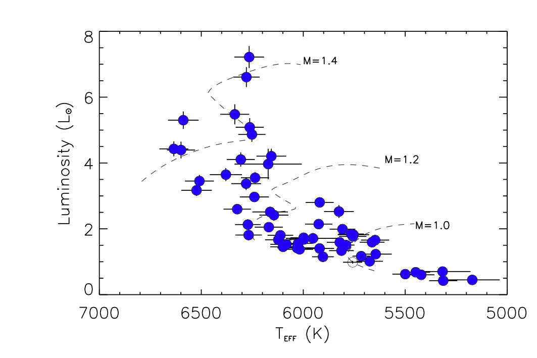 Figure 1
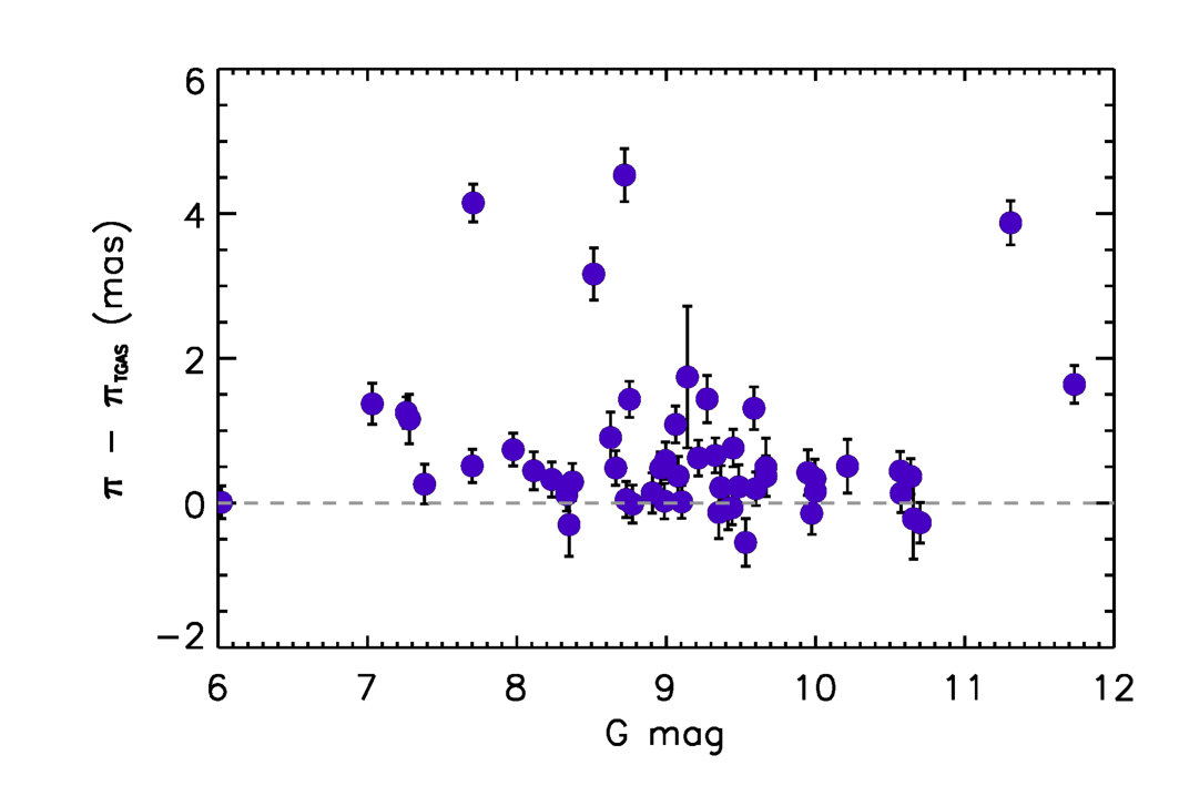 Figure 2
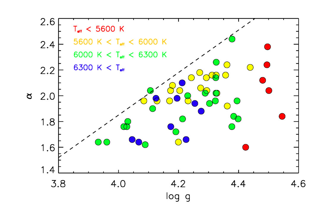 Figure 3
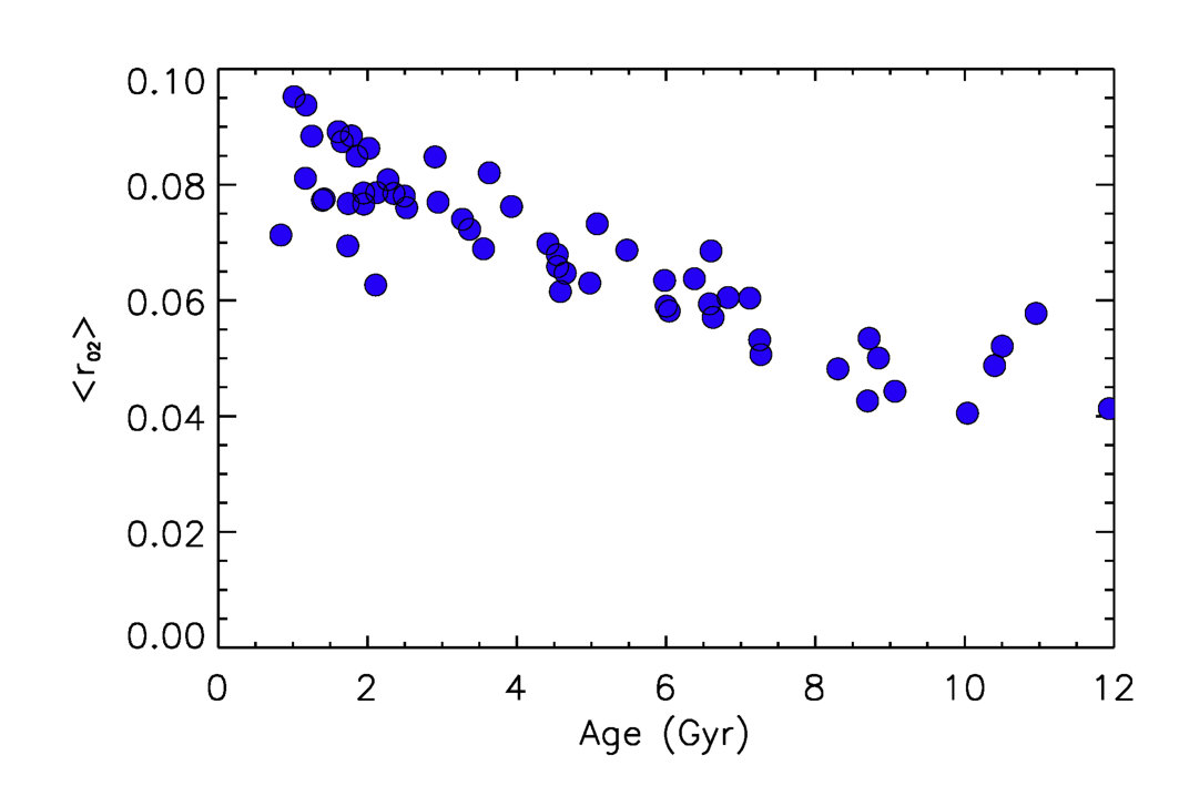 Figure 4
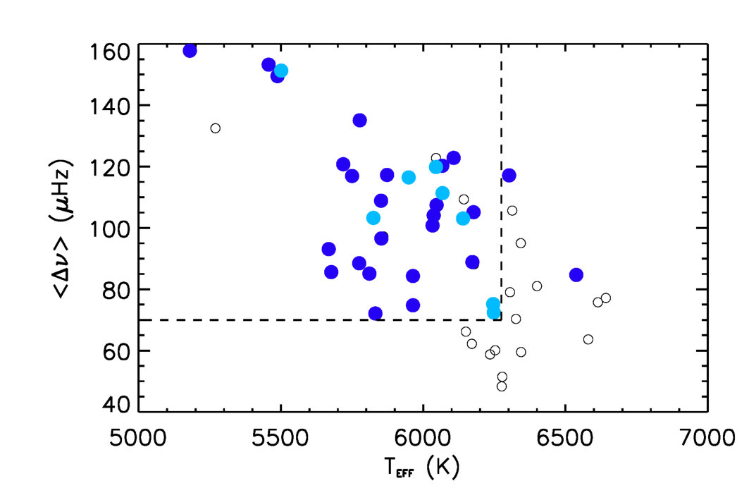 Figure 5
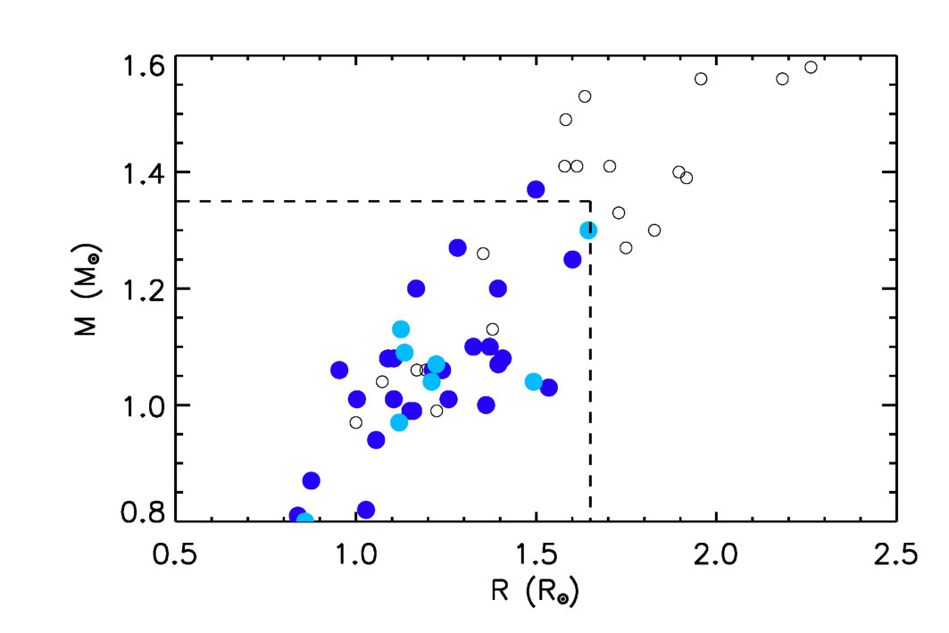 Figure 6
Peer Reviews
No public reviews on file for this paper yet. If you reviewed it on a platform where reviews are public (OpenReview, ICLR, NeurIPS, ICML), you can paste yours below so the community can read it here.
Videos
No videos yet. Explain this paper in a talk, walkthrough, or lecture? Add one.
\wocname
epj \woctitleSeismology of the Sun and the Distant Stars 2016
11institutetext: Université Côte d’Azur, Laboratoire Lagrange, CNRS, Blvd de l’Observatoire, CS 34229, 06304 Nice cedex 4, France 22institutetext: Center for Extrasolar Planetary Systems, Space Science Institute, 4750 Walnut St. Suite 205, Boulder CO 80301, USA 33institutetext: Visiting Scientist, National Solar Observatory, 3665 Discovery Dr., Boulder CO 80303, USA 44institutetext: Laboratoire AIM, CEA/DRF-CNRS, Université Paris 7 Diderot, IRFU/SAp, Centre de Saclay, 91191 Gif-sur-Yvette, France 55institutetext: Center for Space Science, NYUAD Institute, New York University Abu Dhabi, PO Box 129188, Abu Dhabi, UAE 66institutetext: Computational & Information Systems Laboratory, NCAR, P.O. Box 3000, Boulder CO 80307, USA
Seismic inference of 57 stars using full-length Kepler data sets
\firstnameOrlagh \lastnameCreevey\fnsep 11 [email protected]
\firstnameTravis S. \lastnameMetcalfe 2233
\firstnameDavid \lastnameSalabert\fnsep Visiting Scientist at 144
\firstnameSavita \lastnameMathur 22
\firstnameMathias \lastnameSchultheis 11
\firstnameRafael A. \lastnameGarcía 44
\firstnameFrédéric \lastnameThévenin 11
\firstnameMichaël \lastnameBazot 55
\firstnameHaiying \lastnameXu 66
Abstract
We present stellar properties of 57 stars from a seismic inference using full-length data sets from Kepler (mass, age, radius, distances). These stars comprise active stars, planet-hosts, solar-analogs, and binary systems. We validate the distances derived from the astrometric Gaia-Tycho solution. Ensemble analysis of the stellar properties reveals a trend of mixing-length parameter with the surface gravity and effective temperature. We derive a linear relationship with the seismic quantity to estimate the stellar age. Finally, we define the stellar regimes where the Kjeldsen et al (2008) empirical surface correction for 1D model frequencies is valid.
1 Introduction
Time-series analysis of the full-length Kepler data sets of solar-like main sequence and subgiants stars is presented in (Lund2016, ). They identify modes of oscillations for 66 stars. Using the Asteroseismic Modeling Portal, AMP111https://amp.phys.au.dk/, we analyse the individual frequency data from (Lund2016, ) for 57 of these stars and we supplement them with spectroscopic data from (Ramirez2009, ; Buchhave2012, ; Pinsonneault2012, ; Huber2013, ; Chaplin2014, ; Pinsonneault2014, ). In this version of AMP, AMP 1.3, we fit the frequency separation ratios and (Roxburgh2003, ) to determine the optimal models for each star in our sample.
The optimization method in AMP is genetic algorithm (GA) which efficiently samples the full parameter ranges without imposing constraints on unknown parameters, such as the mixing-length parameter or the initial chemical composition. The results of the GA is a dense clustering of models (1000s) around the optimal parameters. We analyse the distribution of these models to determine the stellar properties, such as mass, radius and age, along with their uncertainties. Details of the methods can be found in (Metcalfe2003, ; Metcalfe2009, ; Creevey2016, ), with the most recent reference containing the tables of stellar parameters for the sample of 57 stars presented here. The results are validated using solar data and independent determinations of luminosity, radii, and ages.
In these proceedings we analyse the derived stellar properties of our sample. We compare their predicted distances with the recent solution provided by the Gaia-Tycho analysis (TGAS, (tgas2015, ), Sect. 2). In Section 3 we derive expressions for estimating the mixing-length parameter and the stellar age based on observed properties. Finally, in Section 4 we explore the range of parameters where the correction proposed by (Kjeldsen2008, ) to mimic the so-called surface effect related to seismic data is useful.
2 Asteroseismic distances
We use the stellar luminosity, , constrained from the asteroseismic analysis to compute the stellar distance, as a parallax. The model surface gravity and the observed and [Fe/H] are used to derive the amount of interstellar absorption between the top of the Earth’s atmosphere and the star, , by applying the isochrone method described in (schultheis2014, ). Here, ths subscript refers to the 2MASS filter (2MASS, ). We compute the bolometric correction , using (marigo2008, ) where the solar bolometric magnitude is 4.72 mag. With , , , and we derive the the distance to each of the stars in our sample, and then its parallax.
The TGAS catalogue of stellar parallaxes was recently made available through the first Gaia Data Release (gaiamission, ). A comparison of the parallaxes we derive and these new values is shown in Figure 2. Apart from a few outliers there is an overall good agreement between the independent methods. However, the parallaxes that we derive are systematically larger, with a mean difference of +0.7 mas, just over 2 the current uncertainties on the TGAS parallaxes. The cause of this systematic difference is currently under investigation. Nevertheless it is worthy to note that such comparisons of independent methods may allow us to reveal errors in the extinction measurements, the bolometric corrections, the or the underlying assumptions in the models which compute the stellar luminosities.
3 Trends in stellar properties
Performing a homogenous analysis on a large sample allows us to check for trends in some stellar parameters, and compare them to trends derived or established by other methods. We performed this check for two parameters: the mixing-length parameter and the stellar age.
3.1 The mixing-length parameter versus and
The mixing-length parameter, , is usually calibrated for a solar model and then applied to all models for a set range of masses and metallicities. However, several authors have shown that this approach is not correct (bonaca2012, ; creevey2012A, ). The values of resulting from a GA offer an optimal approach to effectively test and subsequently constrain this parameter, since the only assumption is that lies between 1 and 3.
The distribution of with and (colour-coded, see figure caption) is shown in Fig. 3. We see that for a given value of , the value of has an upper limit, which we can approximate by , and this is denoted by the dashed line in the figure. A regression analysis considering the model values of , \log$$T_{\rm eff} and [M/H] yields:
[TABLE]
with a mean and rms of the residual to the fit of –0.01 0.15. This equation yields a value of for the known solar properties.
These results agree in part with those derived by (magic2015, ), using full 3D radiative hydrodynamic calculations for convective envelopes. These authors also found that increases with and decreases with . Our fit indicates a very small dependence on metallicity while their results finds an opposite and more significant trend with this parameter. Our sample, however, does not span a very large range in [M/H], and the low coefficient is consistent with zero within the error bars.
3.2 Age and
The frequency separation ratios are effective at probing the gradients near the core of the star (Roxburgh2003, ). As the core is most sensitive to nuclear processing, the are a diagnostic of the evolutionary state of the star. Using theoretical models (lebMon2009, ) showed a relationship between the mean value of and the stellar age. That relationship was recently used by (appourchaux2015, ) to estimate the age of KIC 7510397 (HIP 93511). Figure 3 shows the distribution of versus the derived age for the sample of stars studied here. A linear fit to these data leads to the following estimate of the stellar age, , based on
[TABLE]
This is, of course, only valid for the range covered by our sample. Note that when inserting the solar value of Hz, Eq. 2 yields an age of 4.7 Gyr, in agreement with the Sun’s age as determined by other means.
4 Surface Effects
The comparison of the observed oscillation frequencies from the Sun and other stars with model frequencies calculated from 1D stellar models reveals a systematic error in the models which increases with frequency. These are known as surface effects, which arise from incomplete modelling of the near-surface layers and the use of an adiabatic treatment on the stellar oscillation modes. Efforts to improve the stellar modelling is underway, but the application of improved models on a large scale is still out of reach. To alleviate this problem, several authors have advocated for the use of combination frequencies which are insensitive to this systematic offset (Roxburgh2003, ), hence the exclusive use of and in the AMP 1.3 methodology. However, since individual frequencies contain more information than and , some authors have derived simple prescriptions to mitigate the surface effect. One such parametrization is that of (Kjeldsen2008, ) who suggest a simple correction to the individual frequencies in the form of a power law, namely
[TABLE]
where is a fixed value, calibrated by a solar model, is computed from the differences between the observed and model frequencies (Metcalfe2009, ; Metcalfe2014, ), is the observed frequency mode and is the frequency corresponding to the highest amplitude mode, see (Lund2016, ).
The AMP 1.3 methodology uses exclusively and as the seismic constraints, hence our results are insensitive to the surface effects. Using the model frequencies of the best-matched models, we can test how useful Eq. 3 is for different stellar regimes along the main sequence and early sub-giant phase. The interest in testing this becomes apparent when we consider that for many stars we do not have a high enough precision on the frequencies, or a sufficiently large range of radial orders, to use and to effectively constrain the stellar modelling. This is the case for some ground-based observations and for some stars that will be observed by TESS (tess-ricker2015, ), and PLATO (plato-rauer2014, ), where a limited time series of only one to two months may only be available.
In order to test where Eq. 3 is useful, we calculated the residual between the observed oscillation frequencies and the model frequencies corrected for the surface term (Eq. 3): . Then we defined the metric as the median of the square root of the squared residuals:
[TABLE]
for all and all defined in the region of . We find values of that vary between 0.3 and 10 and this variation is anti-correlated with : as becomes more negative the match with the model becomes worse.
We define a subsample of 44 stars with the best fits to and . This subsample in shown in Fig. 4 as open circles for the observed values of and , and the derived values of mass and radius. In these figures the stars represented by the dark blue filled circles have and those represented by the light blue filled circles have . It is evident from the figures that there exists regions of the parameter space where the surface correction proposed by (Kjeldsen2008, ) adequately corrects for the surface term. These regions are highlighted by the dashed lines, defined more conservatively here as , K, Hz and Hz. In physical properties this corresponds to a star with R*⊙, M⊙, and L⊙*, with no apparent evidence of the age or the metallicity playing any role.
5 Conclusions
In these proceedings we used the derived properties of 57 Kepler stars presented in (Creevey2016, ) to predict the star’s parallaxes, to derive an expression relating the mixing-length parameter and the age to observed properties, and to explore the regions of parameters where the proposed surface correction to individual frequencies by (Kjeldsen2008, ) (Eq. 3) is useful. For this latter point, the aim of defining valid regions is to use the correction for data sets where the frequency precision or the range of radial orders is not sufficient for and to constrain the stellar models. This will be the case for some stars that will be observed in low ecliptic latitudes with TESS and for the step-and-stare pointing phases of the PLATO mission.
The parallaxes that we derived in this work were compared to the parallaxes derived from the Tycho-Gaia solution. We found in general a good agreement between our results. The mean differences between our results (ours – theirs) is +0.7 mas and the cause of this error is currently under study. Nevertheless we validate the new parallaxes from (tgas2015, ). This comparison of parallaxes also highlights the ability of these external measurements to allow us to investigate the sources of systematic errors. We believe that in providing a prior on the luminosity, we may even be able to constrain the initial helium abundance in the star. We look forward to the wealth of forthcoming asteroseismic data on bright nearby stars with TESS and PLATO, and the forthcoming Gaia parallaxes with as precision.
The reference list from the paper itself. Each links out to its DOI / PubMed record.
- 1(1) M.N. Lund, V. Silva Aguirre, G.R. Davies, W.J. Chaplin, J. Christensen-Dalsgaard, G. Houdek, T.R. White, T.R. Bedding, W.H. Ball, D. Huber et al., Ap J 835 , 172 (2017), 1612.00436
- 2(2) I. Ramírez, J. Meléndez, M. Asplund, A&A 508 , L 17 (2009)
- 3(3) L.A. Buchhave, D.W. Latham, A. Johansen, M. Bizzarro, G. Torres, J.F. Rowe, N.M. Batalha, W.J. Borucki, E. Brugamyer, C. Caldwell et al., Nature 486 , 375 (2012)
- 4(4) M.H. Pinsonneault, D. An, J. Molenda-Żakowicz, W.J. Chaplin, T.S. Metcalfe, H. Bruntt, Ap JS 199 , 30 (2012), 1110.4456
- 5(5) D. Huber, W.J. Chaplin, J. Christensen-Dalsgaard, R.L. Gilliland, H. Kjeldsen, L.A. Buchhave, D.A. Fischer, J.J. Lissauer, J.F. Rowe, R. Sanchis-Ojeda et al., Ap J 767 , 127 (2013), 1302.2624
- 6(6) W.J. Chaplin, S. Basu, D. Huber, A. Serenelli, L. Casagrande, V. Silva Aguirre, W.H. Ball, O.L. Creevey, L. Gizon, R. Handberg et al., Ap JS 210 , 1 (2014), 1310.4001
- 7(7) M.H. Pinsonneault, Y. Elsworth, C. Epstein, S. Hekker, S. Mészáros, W.J. Chaplin, J.A. Johnson, R.A. García, J. Holtzman, S. Mathur et al., Ap JS 215 , 19 (2014), 1410.2503
- 8(8) I.W. Roxburgh, S.V. Vorontsov, A&A 411 , 215 (2003)