Search for Cosmic-Ray Electron and Positron Anisotropies with Seven Years of Fermi Large Area Telescope Data
Fermi-LAT Collaboration

TL;DR
This study analyzes seven years of Fermi LAT data to search for anisotropies in high-energy cosmic-ray electrons and positrons, setting stringent upper limits and finding no significant anisotropies.
Contribution
It provides the first detailed anisotropy search using nearly seven years of Fermi LAT data with improved event selection and systematic effect considerations.
Findings
No significant anisotropies detected.
Upper limits on dipole anisotropy are among the strongest to date.
Constraints on nearby source contributions are improved.
Abstract
The Large Area Telescope on board the Fermi Gamma-ray Space Telescope has collected the largest ever sample of high-energy cosmic-ray electron and positron events since the beginning of its operation. Potential anisotropies in the arrival directions of cosmic-ray electrons or positrons could be a signature of the presence of nearby sources. We use almost seven years of data with energies above 42 GeV processed with the Pass~8 reconstruction. The present data sample can probe dipole anisotropies down to a level of . We take into account systematic effects that could mimic true anisotropies at this level. We present a detailed study of the event selection optimization of the cosmic-ray electrons and positrons to be used for anisotropy searches. Since no significant anisotropies have been detected on any angular scale, we present upper limits on the dipole anisotropy. The present…
Click any figure to enlarge with its caption.
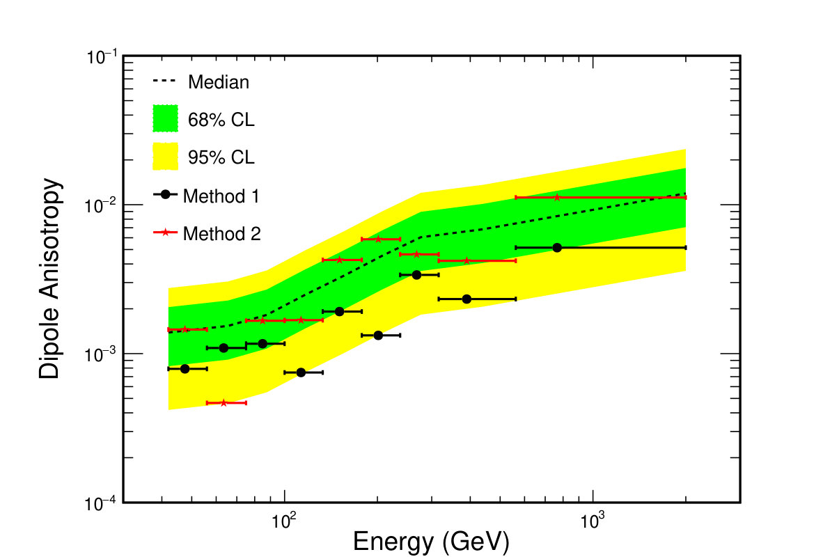 Figure 1
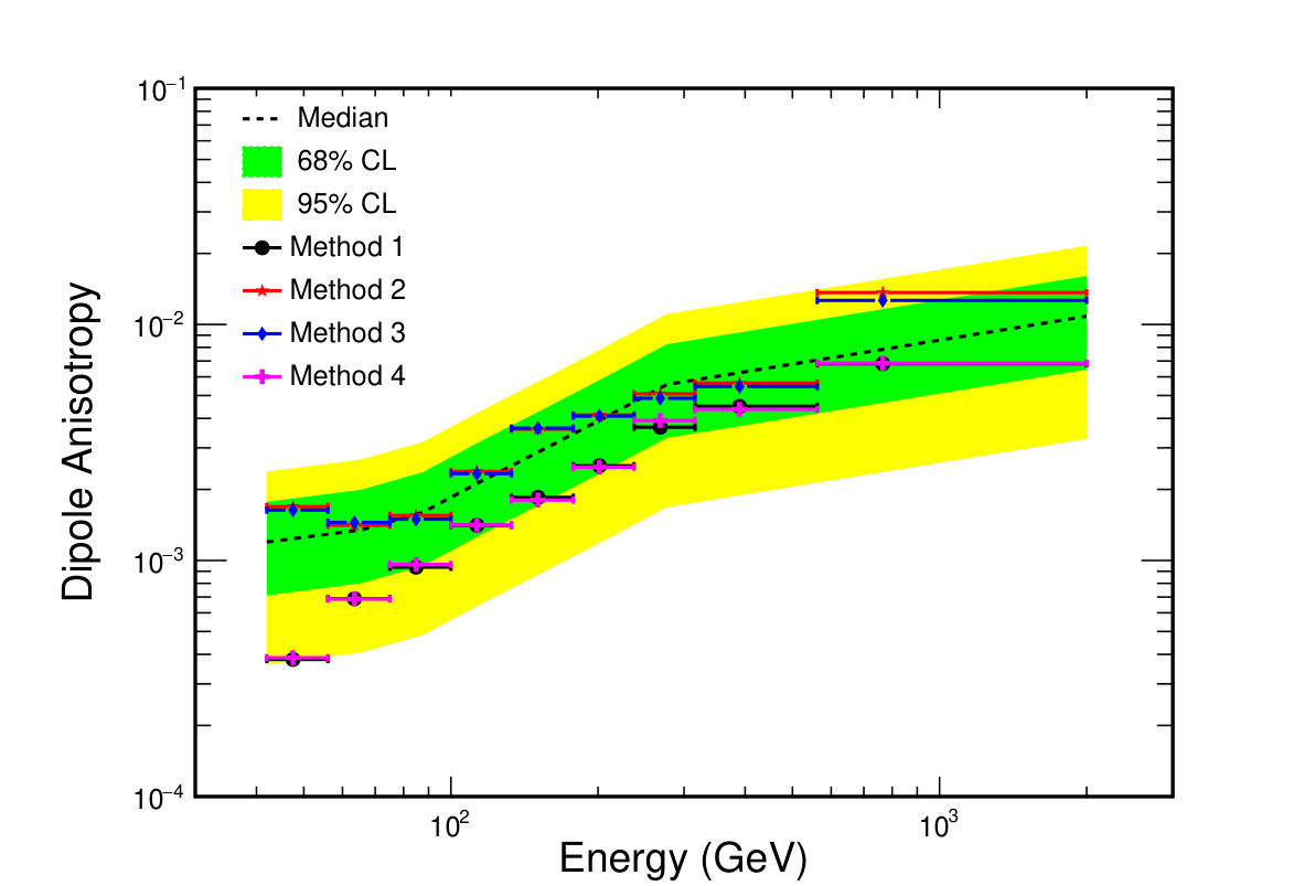 Figure 2
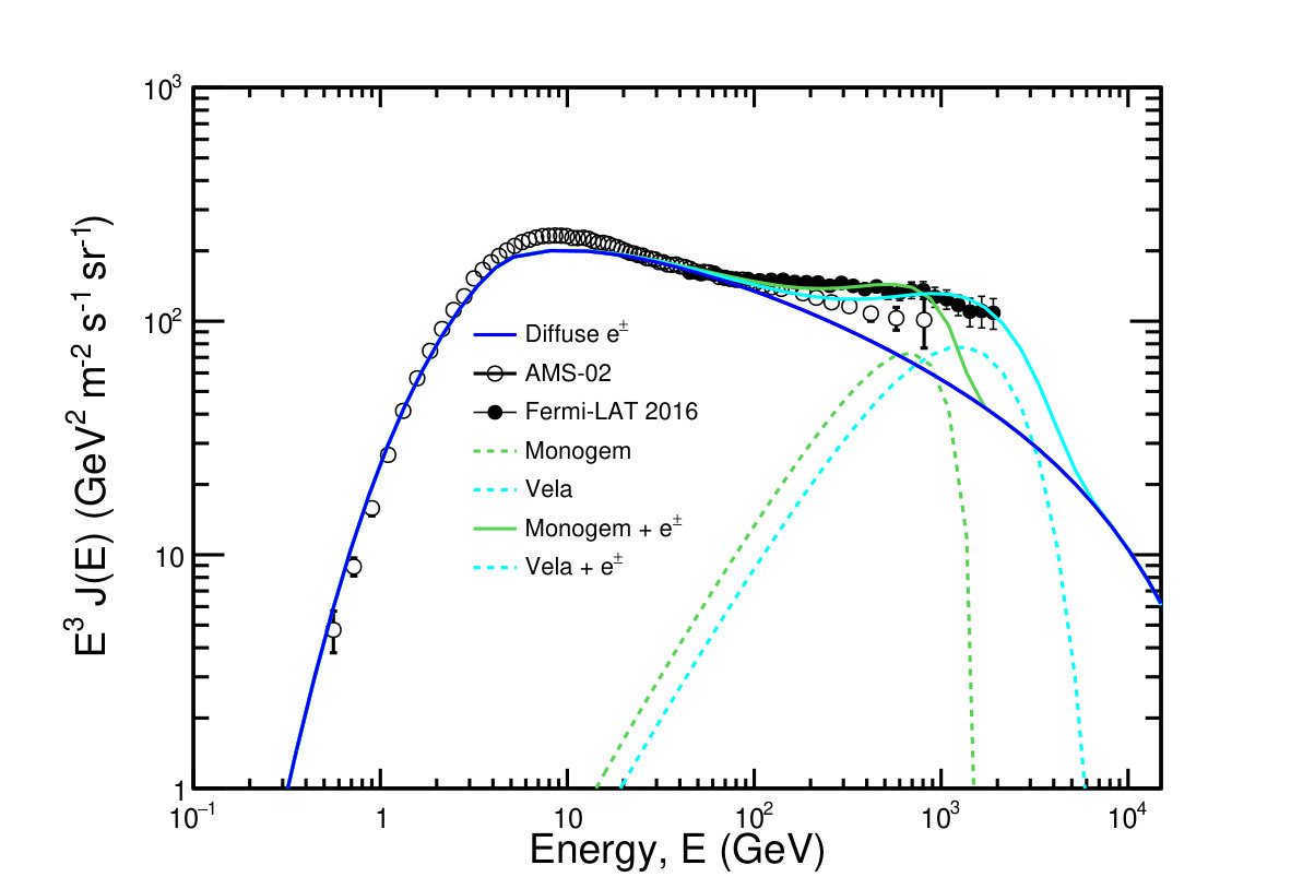 Figure 3
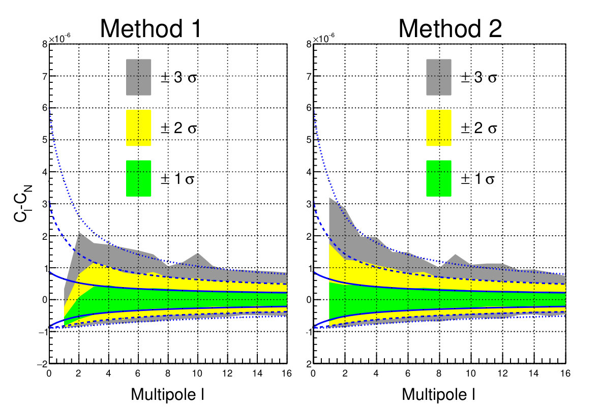 Figure 4
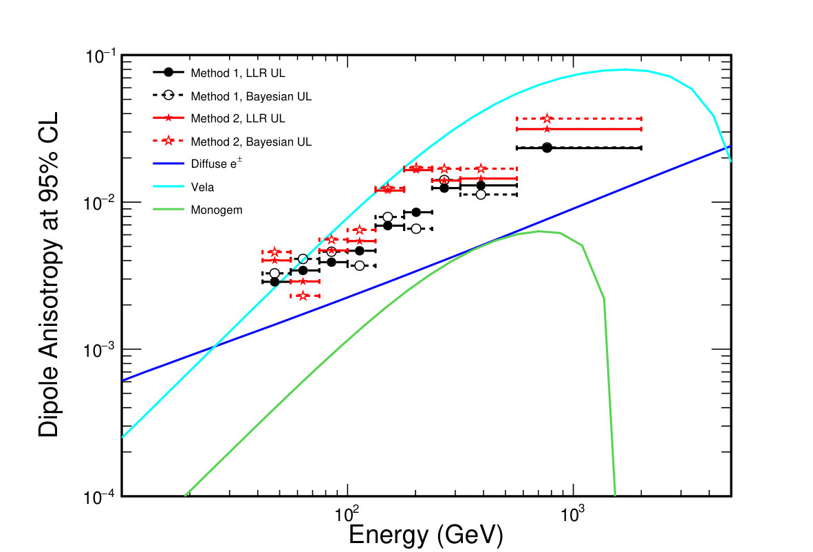 Figure 5
 Figure 6
Peer Reviews
No public reviews on file for this paper yet. If you reviewed it on a platform where reviews are public (OpenReview, ICLR, NeurIPS, ICML), you can paste yours below so the community can read it here.
Videos
No videos yet. Explain this paper in a talk, walkthrough, or lecture? Add one.
The Fermi-LAT collaboration
Search for Cosmic-Ray Electron and Positron Anisotropies with Seven Years of Fermi Large Area Telescope Data
S. Abdollahi
Department of Physical Sciences, Hiroshima University, Higashi-Hiroshima, Hiroshima 739-8526, Japan
M. Ackermann
Deutsches Elektronen Synchrotron DESY, D-15738 Zeuthen, Germany
M. Ajello
Department of Physics and Astronomy, Clemson University, Kinard Lab of Physics, Clemson, South Carolina 29634-0978, USA
A. Albert
Los Alamos National Laboratory, Los Alamos, New Mexico 87545, USA
W. B. Atwood
Santa Cruz Institute for Particle Physics, Department of Physics and Department of Astronomy and Astrophysics, University of California at Santa Cruz, Santa Cruz, California 95064, USA
L. Baldini
Dipartimento di Fisica “Enrico Fermi” dell’Università di Pisa, I-56126 Pisa, Italy
Istituto Nazionale di Fisica Nucleare, Sezione di Pisa, I-56127 Pisa, Italy
G. Barbiellini
Istituto Nazionale di Fisica Nucleare, Sezione di Trieste, I-34127 Trieste, Italy
Dipartimento di Fisica, Università di Trieste, I-34127 Trieste, Italy
R. Bellazzini
Istituto Nazionale di Fisica Nucleare, Sezione di Pisa, I-56127 Pisa, Italy
E. Bissaldi
Dipartimento di Fisica “M. Merlin” dell’Università e del Politecnico di Bari, I-70126 Bari, Italy
Istituto Nazionale di Fisica Nucleare, Sezione di Bari, I-70126 Bari, Italy
E. D. Bloom
W. W. Hansen Experimental Physics Laboratory, Kavli Institute for Particle Astrophysics and Cosmology, Department of Physics and SLAC National Accelerator Laboratory, Stanford University, Stanford, California 94305, USA
R. Bonino
Istituto Nazionale di Fisica Nucleare, Sezione di Torino, I-10125 Torino, Italy
Dipartimento di Fisica, Università degli Studi di Torino, I-10125 Torino, Italy
E. Bottacini
W. W. Hansen Experimental Physics Laboratory, Kavli Institute for Particle Astrophysics and Cosmology, Department of Physics and SLAC National Accelerator Laboratory, Stanford University, Stanford, California 94305, USA
T. J. Brandt
NASA Goddard Space Flight Center, Greenbelt, Maryland 20771, USA
P. Bruel
Laboratoire Leprince-Ringuet, École polytechnique, CNRS/IN2P3, F-91128 Palaiseau, France
S. Buson
NASA Goddard Space Flight Center, Greenbelt, Maryland 20771, USA
M. Caragiulo
Dipartimento di Fisica “M. Merlin” dell’Università e del Politecnico di Bari, I-70126 Bari, Italy
Istituto Nazionale di Fisica Nucleare, Sezione di Bari, I-70126 Bari, Italy
E. Cavazzuti
Agenzia Spaziale Italiana (ASI) Science Data Center, I-00133 Roma, Italy
A. Chekhtman
College of Science, George Mason University, Fairfax, Virginia 22030, USA resident at Naval Research Laboratory, Washington, DC 20375, USA
S. Ciprini
Agenzia Spaziale Italiana (ASI) Science Data Center, I-00133 Roma, Italy
Istituto Nazionale di Fisica Nucleare, Sezione di Perugia, I-06123 Perugia, Italy
F. Costanza
Istituto Nazionale di Fisica Nucleare, Sezione di Bari, I-70126 Bari, Italy
A. Cuoco
Istituto Nazionale di Fisica Nucleare, Sezione di Torino, I-10125 Torino, Italy
Institute for Theoretical Particle Physics and Cosmology, (TTK), RWTH Aachen University, D-52056 Aachen, Germany
S. Cutini
Agenzia Spaziale Italiana (ASI) Science Data Center, I-00133 Roma, Italy
Istituto Nazionale di Fisica Nucleare, Sezione di Perugia, I-06123 Perugia, Italy
F. D’Ammando
INAF Istituto di Radioastronomia, I-40129 Bologna, Italy
Dipartimento di Astronomia, Università di Bologna, I-40127 Bologna, Italy
F. de Palma
Istituto Nazionale di Fisica Nucleare, Sezione di Bari, I-70126 Bari, Italy
Università Telematica Pegaso, Piazza Trieste e Trento, 48, I-80132 Napoli, Italy
R. Desiante
Istituto Nazionale di Fisica Nucleare, Sezione di Torino, I-10125 Torino, Italy
Università di Udine, I-33100 Udine, Italy
S. W. Digel
W. W. Hansen Experimental Physics Laboratory, Kavli Institute for Particle Astrophysics and Cosmology, Department of Physics and SLAC National Accelerator Laboratory, Stanford University, Stanford, California 94305, USA
N. Di Lalla
Dipartimento di Fisica “Enrico Fermi” dell’Università di Pisa, I-56126 Pisa, Italy
Istituto Nazionale di Fisica Nucleare, Sezione di Pisa, I-56127 Pisa, Italy
M. Di Mauro
W. W. Hansen Experimental Physics Laboratory, Kavli Institute for Particle Astrophysics and Cosmology, Department of Physics and SLAC National Accelerator Laboratory, Stanford University, Stanford, California 94305, USA
L. Di Venere
Dipartimento di Fisica “M. Merlin” dell’Università e del Politecnico di Bari, I-70126 Bari, Italy
Istituto Nazionale di Fisica Nucleare, Sezione di Bari, I-70126 Bari, Italy
B. Donaggio
Istituto Nazionale di Fisica Nucleare, Sezione di Padova, I-35131 Padova, Italy
P. S. Drell
W. W. Hansen Experimental Physics Laboratory, Kavli Institute for Particle Astrophysics and Cosmology, Department of Physics and SLAC National Accelerator Laboratory, Stanford University, Stanford, California 94305, USA
C. Favuzzi
Dipartimento di Fisica “M. Merlin” dell’Università e del Politecnico di Bari, I-70126 Bari, Italy
Istituto Nazionale di Fisica Nucleare, Sezione di Bari, I-70126 Bari, Italy
W. B. Focke
W. W. Hansen Experimental Physics Laboratory, Kavli Institute for Particle Astrophysics and Cosmology, Department of Physics and SLAC National Accelerator Laboratory, Stanford University, Stanford, California 94305, USA
Y. Fukazawa
Department of Physical Sciences, Hiroshima University, Higashi-Hiroshima, Hiroshima 739-8526, Japan
S. Funk
Erlangen Centre for Astroparticle Physics, D-91058 Erlangen, Germany
P. Fusco
Dipartimento di Fisica “M. Merlin” dell’Università e del Politecnico di Bari, I-70126 Bari, Italy
Istituto Nazionale di Fisica Nucleare, Sezione di Bari, I-70126 Bari, Italy
F. Gargano
Istituto Nazionale di Fisica Nucleare, Sezione di Bari, I-70126 Bari, Italy
D. Gasparrini
Agenzia Spaziale Italiana (ASI) Science Data Center, I-00133 Roma, Italy
Istituto Nazionale di Fisica Nucleare, Sezione di Perugia, I-06123 Perugia, Italy
N. Giglietto
Dipartimento di Fisica “M. Merlin” dell’Università e del Politecnico di Bari, I-70126 Bari, Italy
Istituto Nazionale di Fisica Nucleare, Sezione di Bari, I-70126 Bari, Italy
F. Giordano
Dipartimento di Fisica “M. Merlin” dell’Università e del Politecnico di Bari, I-70126 Bari, Italy
Istituto Nazionale di Fisica Nucleare, Sezione di Bari, I-70126 Bari, Italy
M. Giroletti
INAF Istituto di Radioastronomia, I-40129 Bologna, Italy
D. Green
Department of Physics and Department of Astronomy, University of Maryland, College Park, Maryland 20742, USA
NASA Goddard Space Flight Center, Greenbelt, Maryland 20771, USA
S. Guiriec
NASA Goddard Space Flight Center, Greenbelt, Maryland 20771, USA
A. K. Harding
NASA Goddard Space Flight Center, Greenbelt, Maryland 20771, USA
T. Jogler
Friedrich-Alexander-Universität, Erlangen-Nürnberg, Schlossplatz 4, 91054 Erlangen, Germany
G. Jóhannesson
Science Institute, University of Iceland, IS-107 Reykjavik, Iceland
T. Kamae
Department of Physics, Graduate School of Science, University of Tokyo, 7-3-1 Hongo, Bunkyo-ku, Tokyo 113-0033, Japan
M. Kuss
Istituto Nazionale di Fisica Nucleare, Sezione di Pisa, I-56127 Pisa, Italy
S. Larsson
Department of Physics, KTH Royal Institute of Technology, AlbaNova, SE-106 91 Stockholm, Sweden
The Oskar Klein Centre for Cosmoparticle Physics, AlbaNova, SE-106 91 Stockholm, Sweden
L. Latronico
Istituto Nazionale di Fisica Nucleare, Sezione di Torino, I-10125 Torino, Italy
J. Li
Institute of Space Sciences (IEEC-CSIC), Campus UAB, E-08193 Barcelona, Spain
F. Longo
Istituto Nazionale di Fisica Nucleare, Sezione di Trieste, I-34127 Trieste, Italy
Dipartimento di Fisica, Università di Trieste, I-34127 Trieste, Italy
F. Loparco
Dipartimento di Fisica “M. Merlin” dell’Università e del Politecnico di Bari, I-70126 Bari, Italy
Istituto Nazionale di Fisica Nucleare, Sezione di Bari, I-70126 Bari, Italy
P. Lubrano
Istituto Nazionale di Fisica Nucleare, Sezione di Perugia, I-06123 Perugia, Italy
J. D. Magill
Department of Physics and Department of Astronomy, University of Maryland, College Park, Maryland 20742, USA
D. Malyshev
Erlangen Centre for Astroparticle Physics, D-91058 Erlangen, Germany
A. Manfreda
Dipartimento di Fisica “Enrico Fermi” dell’Università di Pisa, I-56126 Pisa, Italy
Istituto Nazionale di Fisica Nucleare, Sezione di Pisa, I-56127 Pisa, Italy
M. N. Mazziotta
Istituto Nazionale di Fisica Nucleare, Sezione di Bari, I-70126 Bari, Italy
M. Meehan
Department of Physics, University of Wisconsin-Madison, Madison, Wisconsin 53706, USA
P. F. Michelson
W. W. Hansen Experimental Physics Laboratory, Kavli Institute for Particle Astrophysics and Cosmology, Department of Physics and SLAC National Accelerator Laboratory, Stanford University, Stanford, California 94305, USA
W. Mitthumsiri
Department of Physics, Faculty of Science, Mahidol University, Bangkok 10400, Thailand
T. Mizuno
Hiroshima Astrophysical Science Center, Hiroshima University, Higashi-Hiroshima, Hiroshima 739-8526, Japan
A. A. Moiseev
Department of Physics and Department of Astronomy, University of Maryland, College Park, Maryland 20742, USA
Center for Research and Exploration in Space Science and Technology (CRESST) and NASA Goddard Space Flight Center, Greenbelt, Maryland 20771, USA
M. E. Monzani
W. W. Hansen Experimental Physics Laboratory, Kavli Institute for Particle Astrophysics and Cosmology, Department of Physics and SLAC National Accelerator Laboratory, Stanford University, Stanford, California 94305, USA
A. Morselli
Istituto Nazionale di Fisica Nucleare, Sezione di Roma “Tor Vergata”, I-00133 Roma, Italy
M. Negro
Istituto Nazionale di Fisica Nucleare, Sezione di Torino, I-10125 Torino, Italy
Dipartimento di Fisica, Università degli Studi di Torino, I-10125 Torino, Italy
E. Nuss
Laboratoire Univers et Particules de Montpellier, Université Montpellier, CNRS/IN2P3, F-34095 Montpellier, France
T. Ohsugi
Hiroshima Astrophysical Science Center, Hiroshima University, Higashi-Hiroshima, Hiroshima 739-8526, Japan
N. Omodei
W. W. Hansen Experimental Physics Laboratory, Kavli Institute for Particle Astrophysics and Cosmology, Department of Physics and SLAC National Accelerator Laboratory, Stanford University, Stanford, California 94305, USA
D. Paneque
Max-Planck-Institut für Physik, D-80805 München, Germany
J. S. Perkins
NASA Goddard Space Flight Center, Greenbelt, Maryland 20771, USA
M. Pesce-Rollins
Istituto Nazionale di Fisica Nucleare, Sezione di Pisa, I-56127 Pisa, Italy
F. Piron
Laboratoire Univers et Particules de Montpellier, Université Montpellier, CNRS/IN2P3, F-34095 Montpellier, France
G. Pivato
Istituto Nazionale di Fisica Nucleare, Sezione di Pisa, I-56127 Pisa, Italy
G. Principe
Erlangen Centre for Astroparticle Physics, D-91058 Erlangen, Germany
S. Rainò
Dipartimento di Fisica “M. Merlin” dell’Università e del Politecnico di Bari, I-70126 Bari, Italy
Istituto Nazionale di Fisica Nucleare, Sezione di Bari, I-70126 Bari, Italy
R. Rando
Istituto Nazionale di Fisica Nucleare, Sezione di Padova, I-35131 Padova, Italy
Dipartimento di Fisica e Astronomia “G. Galilei”, Università di Padova, I-35131 Padova, Italy
M. Razzano
Istituto Nazionale di Fisica Nucleare, Sezione di Pisa, I-56127 Pisa, Italy
A. Reimer
Institut für Astro- und Teilchenphysik and Institut für Theoretische Physik, Leopold-Franzens-Universität Innsbruck, A-6020 Innsbruck, Austria
W. W. Hansen Experimental Physics Laboratory, Kavli Institute for Particle Astrophysics and Cosmology, Department of Physics and SLAC National Accelerator Laboratory, Stanford University, Stanford, California 94305, USA
O. Reimer
Institut für Astro- und Teilchenphysik and Institut für Theoretische Physik, Leopold-Franzens-Universität Innsbruck, A-6020 Innsbruck, Austria
W. W. Hansen Experimental Physics Laboratory, Kavli Institute for Particle Astrophysics and Cosmology, Department of Physics and SLAC National Accelerator Laboratory, Stanford University, Stanford, California 94305, USA
C. Sgrò
Istituto Nazionale di Fisica Nucleare, Sezione di Pisa, I-56127 Pisa, Italy
D. Simone
Istituto Nazionale di Fisica Nucleare, Sezione di Bari, I-70126 Bari, Italy
E. J. Siskind
NYCB Real-Time Computing Inc., Lattingtown, New York 11560-1025, USA
F. Spada
Istituto Nazionale di Fisica Nucleare, Sezione di Pisa, I-56127 Pisa, Italy
G. Spandre
Istituto Nazionale di Fisica Nucleare, Sezione di Pisa, I-56127 Pisa, Italy
P. Spinelli
Dipartimento di Fisica “M. Merlin” dell’Università e del Politecnico di Bari, I-70126 Bari, Italy
Istituto Nazionale di Fisica Nucleare, Sezione di Bari, I-70126 Bari, Italy
A. W. Strong
Max-Planck Institut für extraterrestrische Physik, D-85748 Garching, Germany
H. Tajima
Solar-Terrestrial Environment Laboratory, Nagoya University, Nagoya 464-8601, Japan
W. W. Hansen Experimental Physics Laboratory, Kavli Institute for Particle Astrophysics and Cosmology, Department of Physics and SLAC National Accelerator Laboratory, Stanford University, Stanford, California 94305, USA
J. B. Thayer
W. W. Hansen Experimental Physics Laboratory, Kavli Institute for Particle Astrophysics and Cosmology, Department of Physics and SLAC National Accelerator Laboratory, Stanford University, Stanford, California 94305, USA
D. F. Torres
Institute of Space Sciences (IEEC-CSIC), Campus UAB, E-08193 Barcelona, Spain
Institució Catalana de Recerca i Estudis Avançats (ICREA), E-08010 Barcelona, Spain
E. Troja
NASA Goddard Space Flight Center, Greenbelt, Maryland 20771, USA
Department of Physics and Department of Astronomy, University of Maryland, College Park, Maryland 20742, USA
J. Vandenbroucke
Department of Physics, University of Wisconsin-Madison, Madison, Wisconsin 53706, USA
G. Zaharijas
Istituto Nazionale di Fisica Nucleare, Sezione di Trieste, and Università di Trieste, I-34127 Trieste, Italy
Laboratory for Astroparticle Physics, University of Nova Gorica, Vipavska 13, SI-5000 Nova Gorica, Slovenia
S. Zimmer
Département de Physique Nucléaire et Corpuscolaire (DPNC), University of Geneva, CH-1211 Genéve 4, Switzerland https://www-glast.stanford.edu/
Abstract
The Large Area Telescope on board the Fermi Gamma-ray Space Telescope has collected the largest ever sample of high-energy cosmic-ray electron and positron events since the beginning of its operation. Potential anisotropies in the arrival directions of cosmic-ray electrons or positrons could be a signature of the presence of nearby sources. We use almost seven years of data with energies above 42 GeV processed with the Pass 8 reconstruction. The present data sample can probe dipole anisotropies down to a level of . We take into account systematic effects that could mimic true anisotropies at this level. We present a detailed study of the event selection optimization of the cosmic-ray electrons and positrons to be used for anisotropy searches. Since no significant anisotropies have been detected on any angular scale, we present upper limits on the dipole anisotropy. The present constraints are among the strongest to date probing the presence of nearby young and middle-aged sources.
Cosmic Ray Electrons, Anisotropy, Pulsar, SNR, Dark Matter
pacs:
96.50.S-, 95.35.+d
I Introduction
High-energy (GeV–TeV) charged Cosmic Rays (CRs) impinging on the top of the Earth’s atmosphere are believed to be produced in our galaxy, most likely in Supernova Remnants (SNRs). During their journey to our solar system, CRs are scattered on random and irregular components of the Galactic Magnetic Field (GMF), which almost isotropize their direction distribution.
CR electrons and positrons (CREs) rapidly lose energy through synchrotron radiation and inverse Compton collisions with low-energy photons of the interstellar radiation field. As a result, CREs observed with energies of 100 GeV (1 TeV) originated from relatively nearby locations, less than about 1.6 kpc (0.75 kpc) away Ackermann et al. (2010); therefore high-energy CREs could originate from a collection of a few nearby sources Berkey and Shen (1969); Shen (1970); Shen and Mao (1971). Evidence for a local CRE source would be of great relevance for understanding the nature of their production.
The Large Area Telescope (LAT) on board the Fermi Gamma-ray Space Telescope observes the entire sky every 2 orbits (3 hours) when the satellite is operated in the usual “sky-survey mode” Atwood et al. (2009), making it an ideal instrument to search for anisotropies on any angular scale and from any direction in the sky.
In 2010, we published the results of the first CRE anisotropy search in the energy range above 60 GeV using the data collected by the LAT in its first year of operation, with null results Ackermann et al. (2010). In this work, we update our previous search using the data collected over almost 7 years and analyzed with a new CRE event selection (Pass 8) Abdollahi et al. (2017), in a broader energy range from 42 GeV to 2 TeV and improving the analysis methods.
We optimized the analysis to minimize any systematic effect that could mimic a signal, for instance effects of the geomagnetic field. For this purpose, we performed a detailed simulation study of the usual methods for anisotropy searches to check for any possible features or biases on the results. Finally, following our validation studies, we present the results obtained analyzing the LAT data, providing a sensitivity to dipole anisotropy as low as .
II Analysis methods
The starting point to search for anisotropies is the construction of a reference sky map that should be seen by the instrument if the CRE flux was isotropic, and represents the null hypothesis. A comparison of the reference map with the actual map should reveal the presence of any anisotropies in the data.
We perform our studies in Galactic coordinates, and we also use the zenith-centered coordinates to check for any feature due to the geomagnetic field. All maps have been built using the HEALPix pixelization scheme with Gorski et al. (2005).
Since the expected signal is tiny, four data-driven methods are used to create the reference map. These methods mitigate potential systematic uncertainties arising from the calculation of the detector exposure Ackermann et al. (2010).
A set of simulated events can be generated by randomly associating detected event times and instrument angles (“shuffling technique” Ackermann et al. (2010), hereafter Method 1). Starting from the position and orientation of the LAT at a given event time, the sky direction is recalculated using the angles in the LAT frame of another event randomly chosen.
An alternative method is based on the overall rate of events detected in a long time interval (“event rate technique”, hereafter Method 2). Each event is assigned a time randomly chosen from an exponential distribution with the given average rate, and a direction extracted from the actual distribution of off-axis and azimuth angles in the LAT. The sky direction is then evaluated using the pointing history of the LAT. A possible issue in this method concerns the duration of the time interval chosen to calculate the average rate, since it must ensure adequate all-sky exposure coverage, especially in the case of a statistically limited data sample. In fact, the presence of any small/medium angular scale anisotropies in the data would create transient fluctuations in the instantaneous values of as these anisotropies pass through the LAT’s field of view (FoV). However, these anisotropies would have no effect on average values calculated on longer time scale, since they would be averaged out Ackermann et al. (2010); Iuppa and Di Sciascio (2013).
Methods 3 and 4 combine the previous techniques, i.e., one can extract the event time sequence from an exponential distribution with given average rate and assign the angles (, ) from random events (hereafter Method 3), or one can keep the observed times and draw the angles (, ) from the distribution (hereafter Method 4).
We calculate the reference map by dividing the data in subsamples of two-months duration 111It is worth mentioning that the precession period of the Fermi orbit is 55 days., then we add the maps corresponding to each period. Such choice guarantees averaging intervals that are long enough to smear out possible medium/large scale anisotropies but, at the same time, that are short compared to changing data-taking conditions (i.e. solar cycle, any change in the LAT performance, etc.).
Once the reference map is known, a simple pixel-to-pixel comparison with the real map can be performed to search for statistically significant deviations. This method is indeed applied to integrated sky maps, in which each pixel contains the integrated number of events in a given circular region around the pixel itself. In case of an anisotropy with angular scale similar to the integration region, spillover effects are reduced increasing sensitivity Ackermann et al. (2010).
Another strategy is the spherical harmonic analysis of a fluctuation sky map. The fluctuation in each pixel is defined as , where () is the number of events in the pixel in the real (reference) map. The fluctuations map is expanded in the basis of spherical harmonics, producing a set of coefficients , used to build the auto angular power spectrum (APS) An increased power at a multipole corresponds to an anisotropic excess at angular scale .
Any deviation of the APS from Poisson noise will be a hint of anisotropies. The Poisson noise (also known as white or shot noise) is due to the finite number of events in the map, so that . To check whether the observed power spectrum is statistically compatible with the Poisson noise, we tested the null hypothesis against the alternative one , with . The white noise over a full sky observed with uniform exposure is , where is the total number of observed events. To account for a non-uniform exposure map, the white noise is given by Fornasa et al. (2016).
III Event selection
We select time intervals (Good Time Intervals, GTIs) when the LAT is operating in standard sky survey mode outside the South Atlantic Anomaly (SAA) and removing the times when the LAT is oriented at rocking angles exceeding 222Starting from September 2009, the Fermi telescope operated in survey mode with a rocking angle of (against in the first year of operation)..
Assuming an isotropic distribution of CREs at very large distances from the Earth, not all of these particles are able to reach the LAT due to the geomagnetic field and Earth’s occultation. In the case of CREs there are regions where only positrons or electrons are allowed (in the West and in the East, respectively) Ackermann et al. (2012). Therefore, a dedicated selection is employed by means of simulations to reduce the geomagnetic effects on the arrival directions of CREs detected by the LAT. We summarize the results in the next section and the details of our studies are given in Supplementary Material 333See Supplemental Material at the link http://link.aps.org/supplemental/10.1103/PhysRevLett.118.091103 for further information about the data analysis method, the procedure used to optimize the event selection and the calculation of the upper limit of the dipole anisotropy, which includes Refs. Campbell (2015); Li and Ma (1983)..
IV Validation studies
To check the analysis methods and the prediction for the noise of the APS, we developed a simulation of an ideal detector with a FoV radius ranging from to , which includes the real spacecraft position, orientation and livetime of the LAT 444Different FoVs will create different levels of non-uniformity in the exposure map.. We performed 1000 independent realizations with an isotropic event distribution at a rate of 0.1 Hz, covering the same time interval of the current analysis. The simulated event samples are analyzed with the same chain as the real one, and with the same GTI selections described above.
We used the 1000 simulated data sets to check the four analysis methods discussed above. For each realization we applied each method 25 times and we calculated the average reference map. Then we calculated the APS with the anafast code Gorski et al. (2005) by comparing each simulated map with the corresponding reference map.
Figure 1 shows an example of the APS obtained using Methods 1 and 2 for the case of an ideal detector with FoV radius. Further details of this study are presented in Supplementary Material, and the results can be summarized as follows: i) all the methods give the same white noise value: ii) Methods 1 and 4 show some bias with respect to (w.r.t.) the white noise level at low multipoles, comparable with the angular scale of the FoV; iii) Methods 2 and 3 show a better behavior w.r.t. the white noise value. As discussed above, the shuffling technique is based on an event time sequences fixed to the real one, and this can break the Poisson random process between events on an angular scale larger than the FoV.
We performed an additional simulation injecting a dipole anisotropy from the direction with different amplitudes ranging between 10% and 0.1% (expected sensitivity limit due to the statistics). We were able to detect these anisotropies with the shuffling and rate methods in the case of large anisotropy amplitude w.r.t. the sensitivity limit. However, the true dipole anisotropy is underestimated, in particular with the shuffling method. Further details on this validation study can be found in Supplementary Material.
Finally, we performed a further validation study based on the CRE LAT Instrument Response Functions (IRFs) for electrons and protons (which contaminate the CRE sample). We simulated an isotropic distribution with electron, positron and proton intensities according to the AMS02 data Aguilar et al. (2014, 2015), still using the real attitude of the spacecraft with the real LAT livetime. The geomagnetic effects were also taken into account by back-tracking each primary particle from the LAT to 10 Earth radii, to check if it can escape (allowed direction), or if it intercepts the Earth or it is trapped in the geomagnetic field (forbidden direction). We used the International Geomagnetic Reference Field model (IGRF-12) Thébault et al. (2015) to describe the magnetic field in the proximity of the Earth.
We performed the analysis in nine independent energy bins from 42 GeV to 2 TeV. To reduce the geomagnetic effects below the level of our sensitivity, we performed the analysis with a reduced FoV, i.e., we set the allowed maximum off-axis angle as a function of energy. As a result, the maximum zenith angle that could be observed is set by the FoV, since the angle between the LAT Z-axis (on-axis direction) and the zenith (i.e., the rocking angle) is fixed with the sky-survey attitude.
We adopt this strategy to avoid any distortion of the distribution of arrival directions in the instrument coordinates, since in the analysis we assume that this distribution is the same as the one generated by an isotropic arrival distribution. The final set of maximum off-axis () angles are: for E(GeV) in the range [42, 56]; for E(GeV) in the range [56, 75] and for E(GeV)75. The maximum off-axis angle used in the current work corresponds to the one used to reconstruct the LAT CRE spectrum Abdollahi et al. (2017).
We calculate the APS with the four methods introduced above. For each method we average 10000 realizations to create the reference map to be used to extract the APS.
Figure 2 shows the dipole anisotropy Ackermann et al. (2010) calculated using the values as a function of energy for the last simulation for Methods 1-4 (top panel). The colored bands show the expected confidence intervals due to the white noise, i.e., assuming the null hypothesis , and correspond to the 68% and 95% central confidence intervals of . Methods 1 and 4 underestimate the white noise level, in particular for the low energy bins (i.e., those with smaller FoVs), still in the expected band, while Method 2 and 3 show a better behavior. These results are similar to those discussed in the case of ideal detectors with different FoVs. Further details are discussed in the SOM. Given the compatibility of the results of Method 1 with 4 and Method 2 with 3 we decided to analyze data using only Method 1 and 2 555We decided to use these two methods for a consistency check despite introducing many trials in the analysis chain and reducing the post-trials significance in case of any detections..
V Data analysis and discussion
We performed the analysis on real data in nine independent energy bins with energy-dependent FoVs as discussed above, on a total of about 12.2M (52k) of events above 42 (562) GeV.
We present in the SOM the maps for the various energy bins in zenith-centered and Galactic coordinates. We also show the significance maps in Galactic coordinates obtained by comparing the integrated reference maps produced with Method 2 to the actual integrated maps. The significances shown in these maps are pre-trials, i.e., they do not take into account the correlations between adjacent pixels (see. Ackermann et al. (2010) for a full discussion). In any case, none of these maps indicates significant excesses or deficits at any angular scale, showing that our measurements are consistent with an isotropic sky.
We have calculated the APS for real data with Method 1 and 2 for the nine energy bins (see Figs. [15] and [16] of the SOM). The current results lie within the 3 range of the expected white noise up to angular scale of a few degrees, showing the consistency with an isotropic sky for all energy bins tested and for . In particular, Fig. 2 (bottom panel) shows the dipole anisotropy as a function of energy calculated from the evaluated with Methods 1 and 2. Since no significant anisotropies have been detected, we calculate upper limits on the dipole anisotropy (Fig. 3).
The current results can be compared with the expected anisotropy from Galactic CREs. Figure 3 (top panel) shows the spectrum of the Galactic CREs component evaluated with the DRAGON propagation code (2D version) Evoli et al. (2008) with secondary particles production from Ref. Mazziotta et al. (2016), assuming that the scalar diffusion coefficient depends on the particle rigidity and on the distance from the Galactic plane according to the parametrization , where , 4 GV and 4 kpc. The Alfvén velocity is set to . In the same figure, the intensity expected from individual sources located in the Vela (290 pc distance and 1.1 yr age) and Monogem (290 pc distance and yr age) positions are also shown. For the single sources, we have adopted a burst-like electron injection spectrum in which the duration of the emission is much shorter than the travel time from the source, described by a power law with index and with an exponential cut-off =1.1 TeV, i.e., (see Refs. Ackermann et al. (2010); Grasso et al. (2009)) 666The solar modulation was treated using the force-field approximation with =0.62 GV Gleeson and Axford (1968).. For both sources, the value of the normalization constant has been chosen to obtain a total flux not higher than that measured by the Fermi-LAT Abdollahi et al. (2017) and by AMS02 Aguilar et al. (2014). Possible effects of the regular magnetic field on the predicted dipole are not considered here (see Ahlers (2016)).
Figure 3 shows the upper limits (UL) at 95% CL on the dipole anisotropy as a function of energy. We calculate the ULs using the frequentist (log-likelihood ratio, LLR) and Bayesian methods. The current ULs as a funtion of energy at 95%CL range from to , of a factor of about 3 better than the previous results 777We point out that the current limits on the dipole anisotropies have been calculated in independent energy bins, while in Ref. Ackermann et al. (2010) they were calculated as a function of minimum energy. In addition, the current methodology to calculate the ULs is different w.r.t. the one used in Ref. Ackermann et al. (2010) (see SOM).
In Fig. 3 the anisotropy due to the Galactic CREs is also shown, together with the one expected from Vela and Monogem sources based on the same models used for estimating potential spectral contributions from them Grasso et al. (2009). The current limits on the dipole anisotropy are probing nearby young and middle-aged sources.
The current results on the CRE anisotropy with the measurements of their spectra can constrain the production of these particles in Supernova Remnants and Pulsar Wind Nebulae Di Bernardo et al. (2011); Linden and Profumo (2013); Manconi et al. (2016) or from dark matter annihilation Cernuda (2010); Borriello et al. (2012).
The Heliospheric Magnetic Field (HMF) can also affect the directions of CREs, but it is not easy to quantify its effect. A dedicated analysis in ecliptic coordinates would be sensitive to HMF effects. However, such analysis was performed with 1 year of CRE data above 60 GeV to constrain dark matter models without finding any significant feature Ajello et al. (2011).
Anisotropy that is not associated with the direction to nearby CR sources is expected to result from the Compton-Getting (CG) effect Compton and Getting (1935), in which the relative motion of the observer w.r.t the CR plasma changes the intensity of the CR fluxes, with larger intensity arriving from the direction of motion and lower intensity arriving from the opposite direction. The expected amplitude of these motions is less than , smaller than the sensitivity of this search.
Contamination of the CRE sample with other species (protons) can introduce some systematic uncertainties in the measurement. Ground experiments have detected anisotropies for protons of energies above 10 TeV at the level. These anisotropies decrease with decreasing energies, and since the proton contamination in our CRE selection is about 10% Abdollahi et al. (2017), the total anisotropy from proton contamination is expected to be less than , much smaller than the current sensitivity. Moreover, being , including the proton contamination would increase the measured limits by a factor , where is the contamination. Such an increase would be noticeable only in the highest-energy bin and can be quantified to .
Acknowledgements.
VI Acknowledgments
The Fermi LAT Collaboration acknowledges generous ongoing support from a number of agencies and institutes that have supported both the development and the operation of the LAT as well as scientific data analysis. These include the National Aeronautics and Space Administration and the Department of Energy in the United States, the Commissariat à l’Energie Atomique and the Centre National de la Recherche Scientifique / Institut National de Physique Nucléaire et de Physique des Particules in France, the Agenzia Spaziale Italiana and the Istituto Nazionale di Fisica Nucleare in Italy, the Ministry of Education, Culture, Sports, Science and Technology (MEXT), High Energy Accelerator Research Organization (KEK) and Japan Aerospace Exploration Agency (JAXA) in Japan, and the K. A. Wallenberg Foundation, the Swedish Research Council and the Swedish National Space Board in Sweden.Additional support for science analysis during the operations phase is gratefully acknowledged from the Istituto Nazionale di Astrofisica in Italy and the Centre National d’Études Spatiales in France.
The authors acknowledge the use of HEALPix http://healpix.sourceforge.net described in K.M. Gorski et al., 2005, Ap.J., 622, p.759. S. B. and S. G acknowledges support as a NASA Postdoctoral Program Fellow, USA. M.R. acknowledges funded by contract FIRB-2012-RBFR12PM1F from the Italian Ministry of Education, University and Research (MIUR).
The authors acknowledge the use of HEALPix http://healpix.sourceforge.net described in K.M. Gorski et al., 2005, Ap.J., 622, p.759
The reference list from the paper itself. Each links out to its DOI / PubMed record.
- 1Ackermann et al. (2010) M. Ackermann et al. (Fermi-LAT Collaboration), Phys. Rev. D 82 , 092003 (2010) , ar Xiv:1008.5119 [astro-ph.HE] . · doi ↗
- 2Berkey and Shen (1969) G. B. Berkey and C. S. Shen, Phys. Rev. 188 , 1994 (1969) . · doi ↗
- 3Shen (1970) C. S. Shen, Astrophys. J. Letter 162 , L 181 (1970) . · doi ↗
- 4Shen and Mao (1971) C. S. Shen and C. Y. Mao, Astrophys. J. Letter 9 , 169 (1971) .
- 5Atwood et al. (2009) W. B. Atwood et al. (Fermi-LAT Collaboration), Astrophys. J. 697 , 1071 (2009) , ar Xiv:0902.1089 [astro-ph.IM] . · doi ↗
- 6Abdollahi et al. (2017) S. Abdollahi et al. (Fermi-LAT Collaboration), To be published (2017).
- 7Gorski et al. (2005) K. M. Gorski, E. Hivon, A. J. Banday, B. D. Wandelt, F. K. Hansen, M. Reinecke, and M. Bartelman, Astrophys. J. 622 , 759 (2005) , ar Xiv:astro-ph/0409513 [astro-ph] . · doi ↗
- 8Iuppa and Di Sciascio (2013) R. Iuppa and G. Di Sciascio, Astrophys. J. 766 , 96 (2013) , ar Xiv:1301.1833 [astro-ph.IM] . · doi ↗