Integrated Linear Reconstruction for Finite Volume Scheme on Arbitrary Unstructured Grids
Li Chen, Guanghui Hu, Ruo Li

TL;DR
This paper introduces an improved integrated linear reconstruction method for finite volume schemes on arbitrary unstructured grids, removing previous geometric restrictions and ensuring positivity-preserving properties.
Contribution
The paper presents a new convex quadratic programming-based reconstruction approach that satisfies the local maximum principle on arbitrary unstructured meshes without geometric constraints.
Findings
Ensures local maximum principle on arbitrary unstructured grids.
Reconstruction is parameter-free and efficient.
Finite volume scheme remains positivity-preserving for Euler equations.
Abstract
In [L. Chen and R. Li, Journal of Scientific Computing, Vol. 68, pp. 1172--1197, (2016)], an integrated linear reconstruction was proposed for finite volume methods on unstructured grids. However, the geometric hypothesis of the mesh to enforce a local maximum principle is too restrictive to be satisfied by, for example, locally refined meshes or distorted meshes generated by arbitrary Lagrangian-Eulerian methods in practical applications. In this paper, we propose an improved integrated linear reconstruction approach to get rid of the geometric hypothesis. The resulting optimization problem is a convex quadratic programming problem, and hence can be solved efficiently by classical active-set methods. The features of the improved integrated linear reconstruction include that i). the local maximum principle is fulfilled on arbitrary unstructured grids, ii). the reconstruction is…
Click any figure to enlarge with its caption.
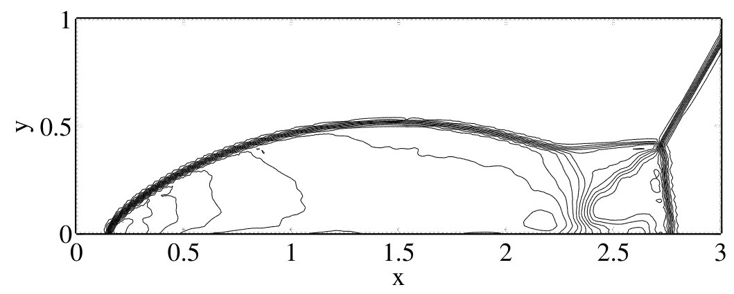 Figure 1
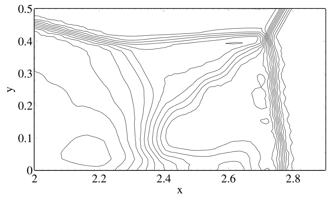 Figure 2
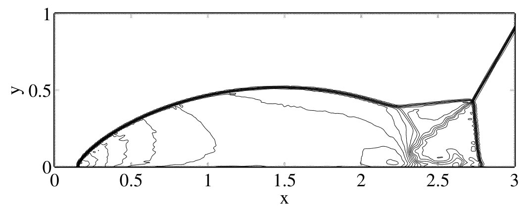 Figure 3
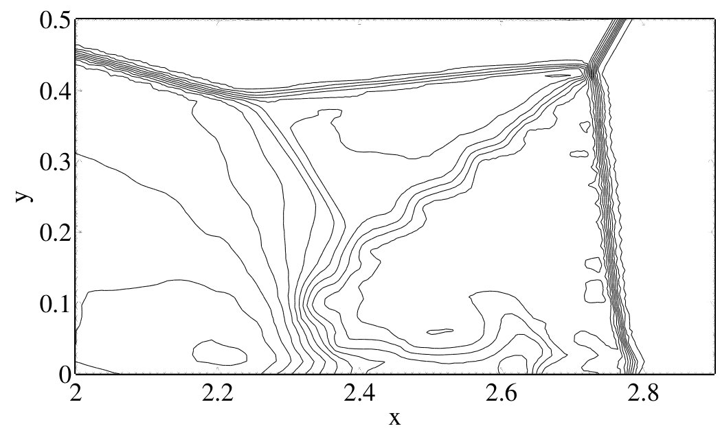 Figure 4
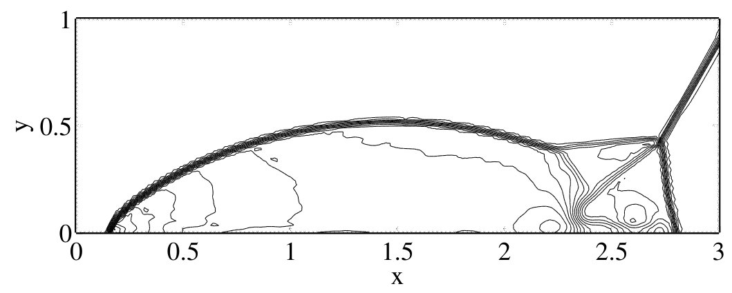 Figure 5
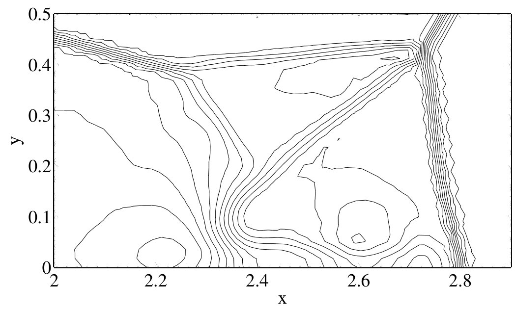 Figure 6
 Figure 7
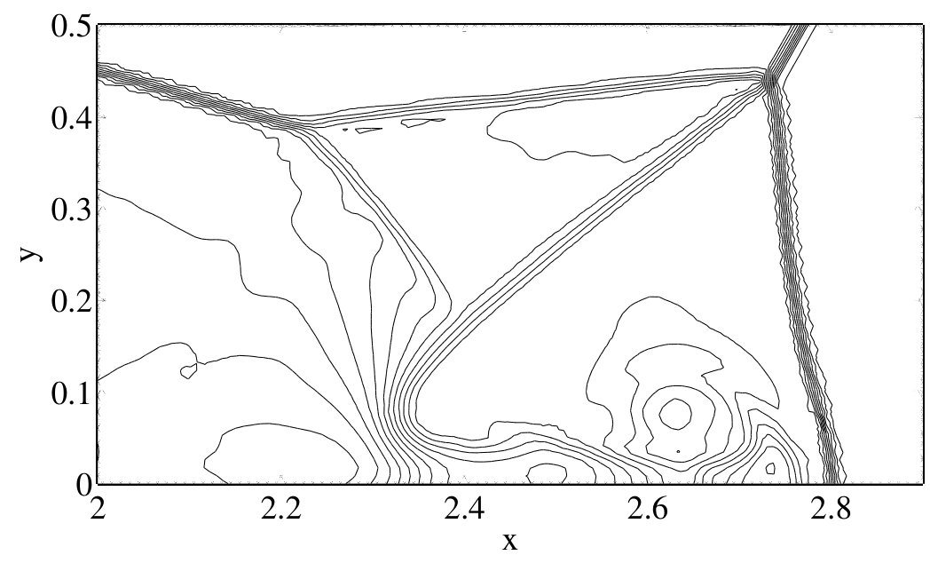 Figure 8
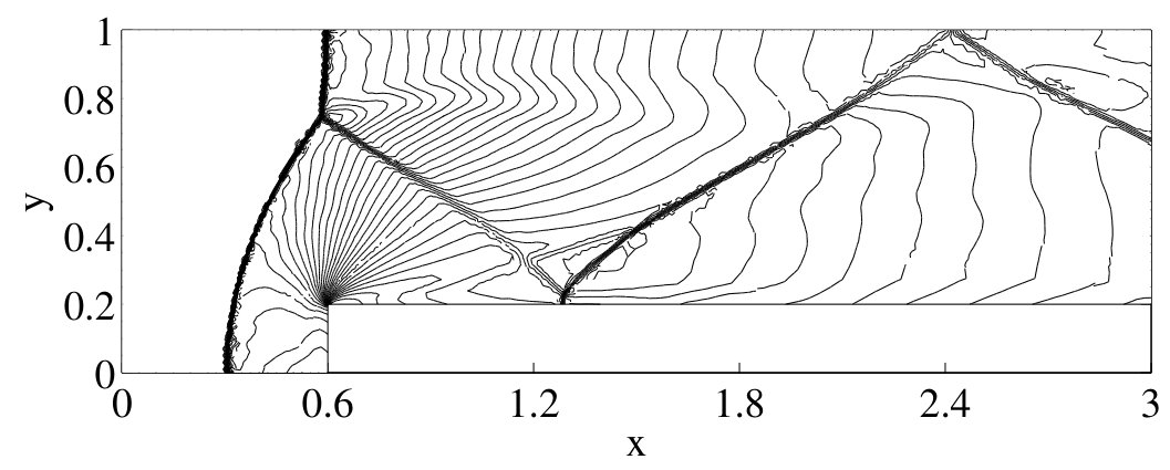 Figure 9
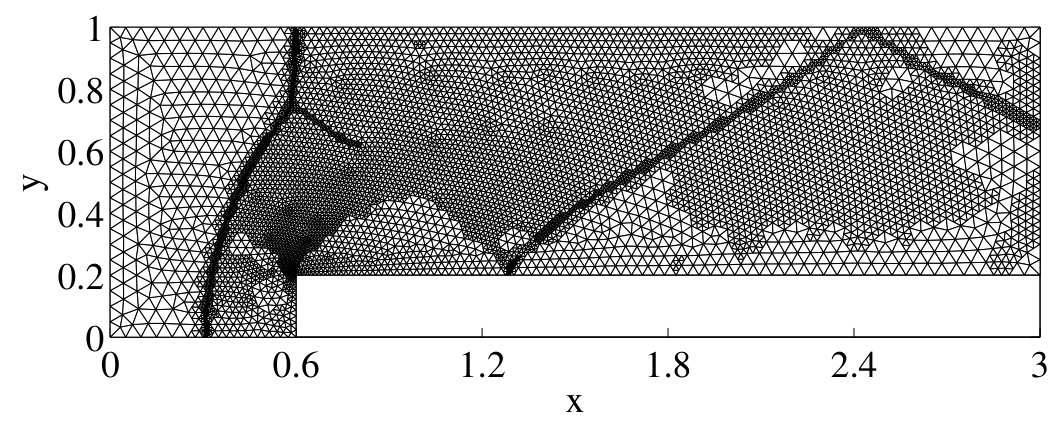 Figure 10
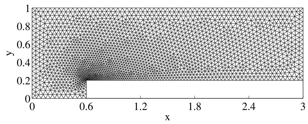 Figure 11
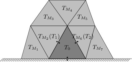 Figure 12
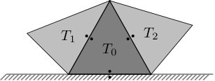 Figure 13
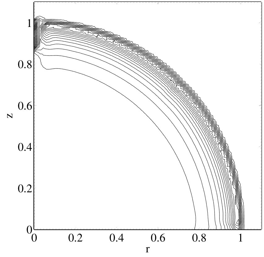 Figure 14
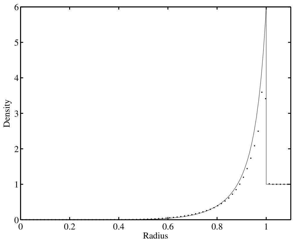 Figure 15
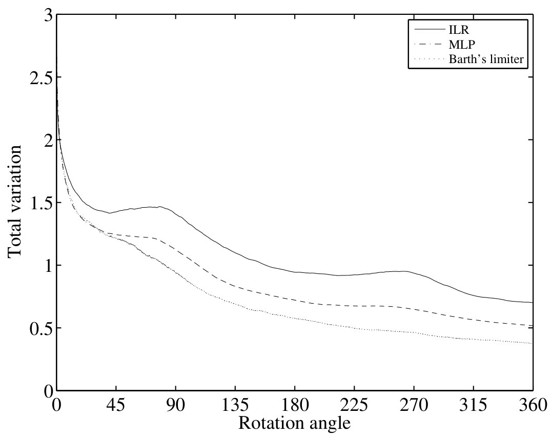 Figure 16
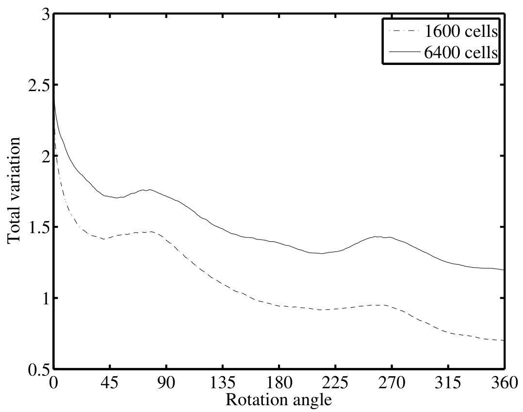 Figure 17
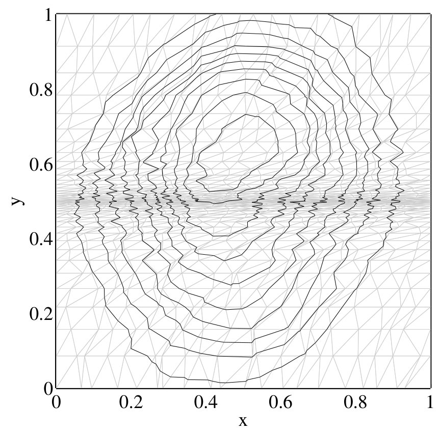 Figure 18
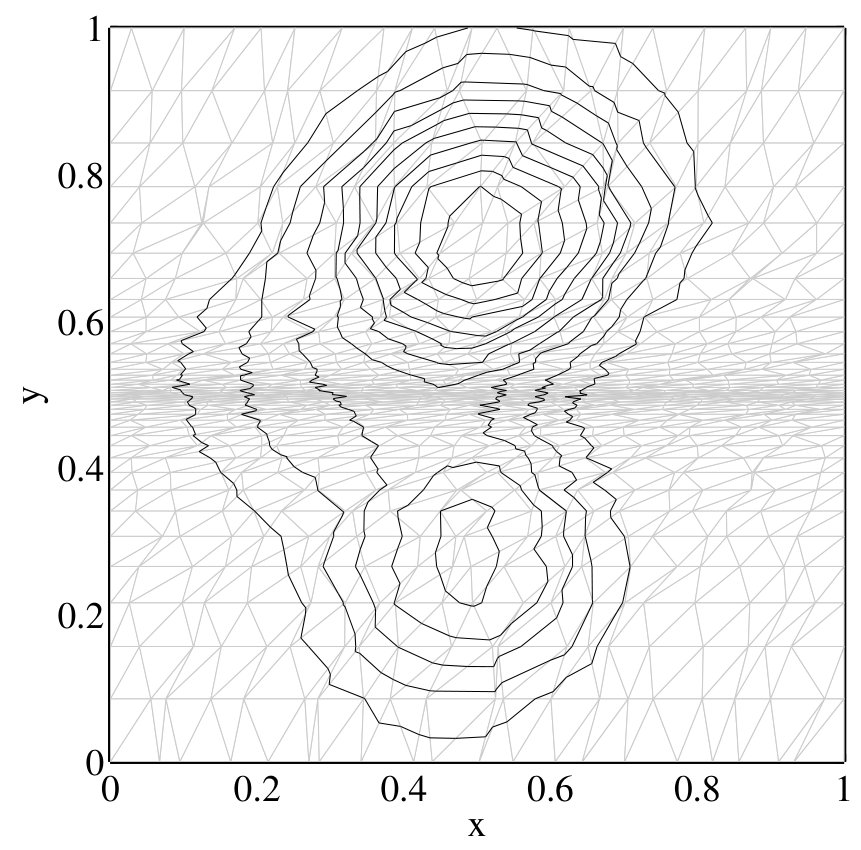 Figure 19
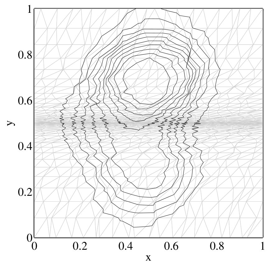 Figure 20
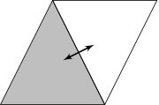 Figure 1
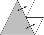 Figure 2
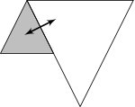 Figure 3
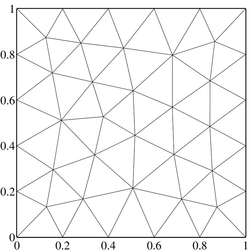 Figure 24
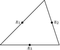 Figure 1
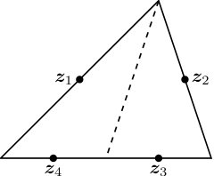 Figure 2
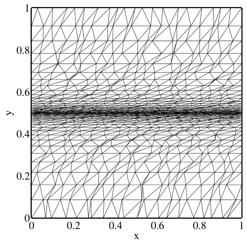 Figure 27
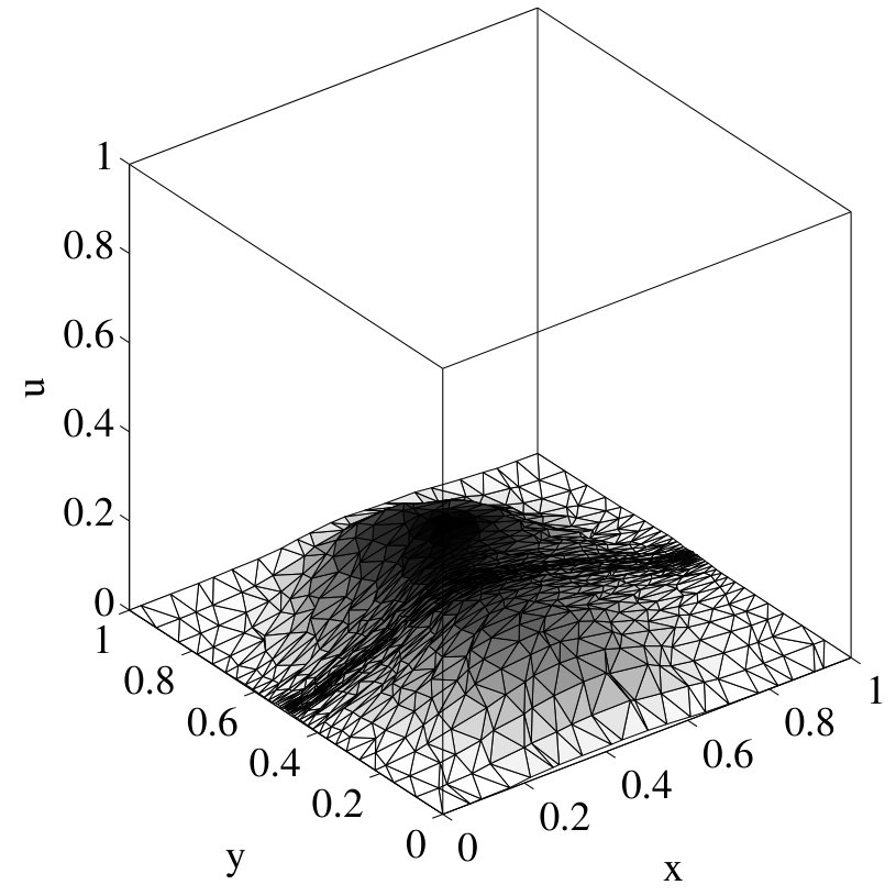 Figure 28
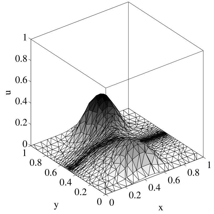 Figure 29
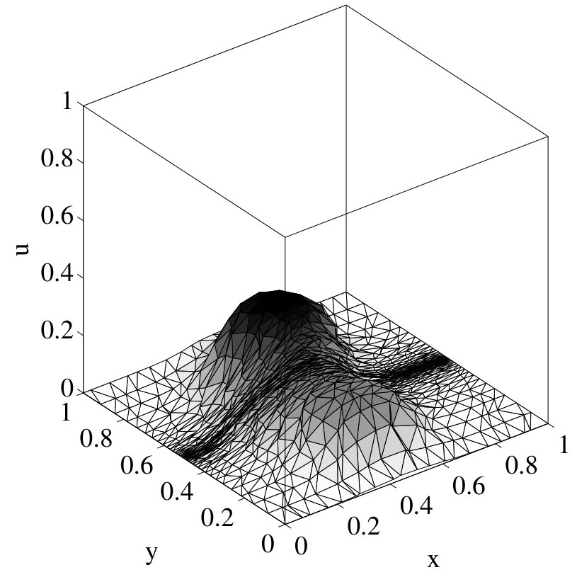 Figure 30
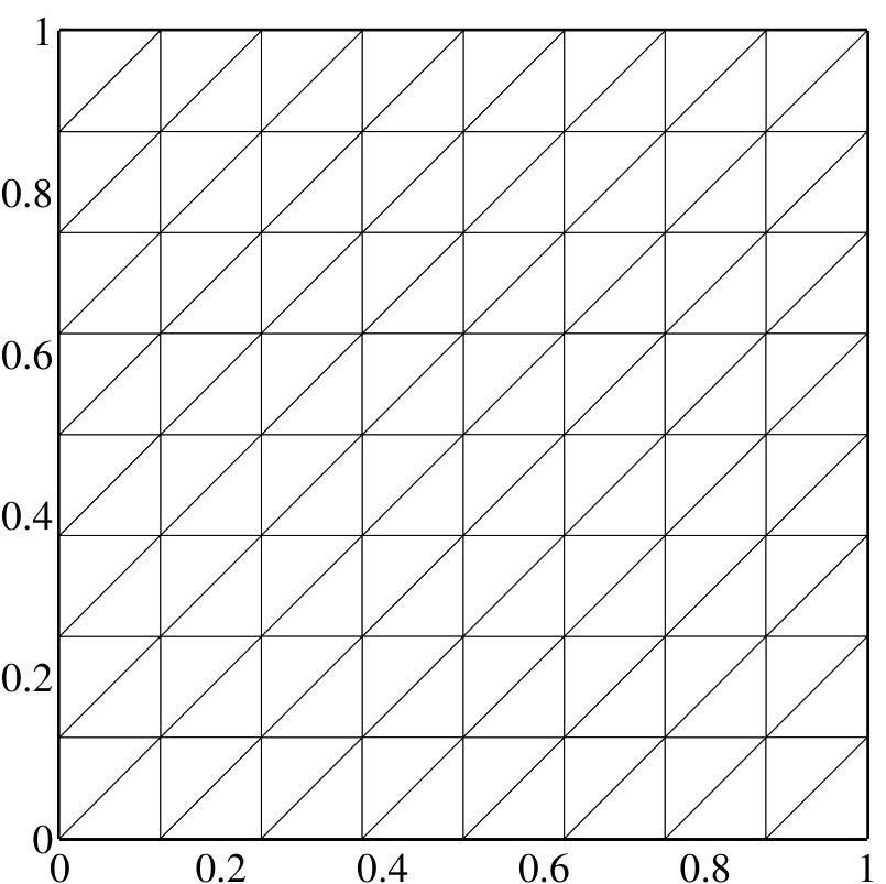 Figure 31
| Cells | error | Order | error | Order | Reconstruction cost (s) | |
|---|---|---|---|---|---|---|
| ILR | 16162 | 4.06e-2 | 2.33 | 1.71e-1 | 1.45 | 1 |
| 32322 | 1.16e-2 | 1.81 | 6.35e-2 | 1.43 | 7 | |
| 64642 | 3.28e-3 | 1.82 | 3.00e-2 | 1.08 | 64 | |
| 1281282 | 8.61e-4 | 1.93 | 1.23e-2 | 1.28 | 444 | |
| MLP | 16162 | 6.19e-2 | 1.96 | 2.54e-1 | 1.13 | 1 |
| 32322 | 1.32e-2 | 2.23 | 9.70e-2 | 1.39 | 6 | |
| 64642 | 2.69e-3 | 2.29 | 3.45e-2 | 1.49 | 51 | |
| 1281282 | 5.71e-4 | 2.24 | 1.19e-2 | 1.54 | 392 | |
| Barth’s limiter | 16162 | 1.36e-1 | 1.22 | 4.25e-1 | 0.82 | 1 |
| 32322 | 7.26e-2 | 0.90 | 2.65e-1 | 0.68 | 3 | |
| 64642 | 3.46e-2 | 1.07 | 1.40e-1 | 0.92 | 29 | |
| 1281282 | 1.82e-2 | 0.93 | 9.93e-2 | 0.50 | 231 | |
| Unlimited | 16162 | 3.40e-2 | 2.17 | 7.51e-2 | 2.01 | 1 |
| 32322 | 7.63e-3 | 2.16 | 1.69e-2 | 2.15 | 3 | |
| 64642 | 1.85e-3 | 2.05 | 3.94e-3 | 2.10 | 27 | |
| 1281282 | 4.58e-4 | 2.01 | 9.48e-4 | 2.05 | 203 |
Peer Reviews
No public reviews on file for this paper yet. If you reviewed it on a platform where reviews are public (OpenReview, ICLR, NeurIPS, ICML), you can paste yours below so the community can read it here.
Videos
No videos yet. Explain this paper in a talk, walkthrough, or lecture? Add one.
\emails
[email protected] (L. Chen), [email protected] (G.H. Hu), [email protected] (R. Li)
Integrated Linear Reconstruction for Finite Volume Scheme on
Arbitrary Unstructured Grids
Li Chen
1
Guanghui Hu\corrauth
2,3
and Ruo Li
4
11affiliationmark: School of Mathematical Sciences, Peking University, Beijing, China
22affiliationmark: Department of Mathematics, University of Macau, Macao SAR, China
33affiliationmark: UM Zhuhai Research Institute, Zhuhai, Guangdong, China
44affiliationmark: HEDPS & CAPT, LMAM & School of Mathematical Sciences, Peking University, Beijing, China
Abstract
In [L. Chen and R. Li, Journal of Scientific Computing, Vol. 68, pp. 1172–1197, (2016)], an integrated linear reconstruction was proposed for finite volume methods on unstructured grids. However, the geometric hypothesis of the mesh to enforce a local maximum principle is too restrictive to be satisfied by, for example, locally refined meshes or distorted meshes generated by arbitrary Lagrangian-Eulerian methods in practical applications. In this paper, we propose an improved integrated linear reconstruction approach to get rid of the geometric hypothesis. The resulting optimization problem is a convex quadratic programming problem, and hence can be solved efficiently by classical active-set methods. The features of the improved integrated linear reconstruction include that i). the local maximum principle is fulfilled on arbitrary unstructured grids, ii). the reconstruction is parameter-free, and iii). the finite volume scheme is positivity-preserving when the reconstruction is generalized to the Euler equations. A variety of numerical experiments are presented to demonstrate the performance of this method.
keywords:
linear reconstruction; finite volume method; local maximum principle; positivity-preserving; quadratic programming
\ams
65M08, 65M50, 76M12, 90C20
1 Introduction
The high-order finite volume schemes can be summarized by a reconstruct-evolve-average (REA) process, i.e. a piecewise polynomial is reconstructed in each cell with given cell averages, then the governing equation is evolved according to those polynomials, and finally the cell averages are recalculated. Among these three stages, reconstruction plays an important role in giving high-order solutions without numerical oscillations. Nowadays, second-order methods have been the workhorse for computational fluid dynamics [1]. To achieve second-order accuracy, a prediction of the gradient is obtained first. Due to the possible non-physical flow caused by the underestimation or overestimation of the gradient, it is necessary to limit the gradient in a proper way, and thus the prediction-limiting algorithm arises. In one-dimensional case, total variation diminishing (TVD) limiters are commonly used in designing high-resolution schemes for conservation laws. Unfortunately, it is very difficult to implement the TVD limiter for multi-dimensional problems, especially on unstructured grids. To get around this negative result, a new class of positive schemes has been proposed [2] which ensures a local maximum principle. Since the introduction of this idea, a large number of limiters have then been developed. These limiters include, among others, the Barth’s limiter [3], the Liu’s limiter [4], the maximum limited gradient (MLG) limiter [5] and the projected limited central difference (PLCD) limiter [6]. See [6] for a comprehensive comparison of these limiters. More recently, Park et al. successfully extended the multi-dimensional limiting process (MLP) introduced in [7] from structured grids to unstructured grids [8]. Li et al. proposed the weighted biased averaging procedure (WBAP) limiter [9] based upon the biased averaging procedure (BAP) limiter which was introduced in [10]. Towards the positivity-preserving property, which is crucial for the stability on solving the Euler equations, there have also been several pioneering works. For instance, Perthame and Shu [11] developed a general finite volume framework on preserving the positivity of density and pressure when solving the Euler equations. Motivated by this work, the framework was extended to the discontinuous Galerkin method on rectangular meshes [12] and on triangular meshes [13], and to the Runge-Kutta discontinuous Galerkin method [14]. More recently, a parametrized limiting technique was proposed in [15] to preserve the positivity property on solving the Euler equations on unstructured grids.
Besides the above prediction-limiting algorithm in the reconstruction, there are also methods which deliver the limited gradient in a single process. For example, Chen and Li [16] introduced the concept of integrated linear reconstruction (ILR), in which the limited gradient is computed by solving a linear programming on each cell using an efficient iterative method. A similar approach was given by May and Berger [17]. However, the fulfillment of local maximum principle of these methods requires certain geometric hypothesis on the grids [16]. Buffard and Clain [18] considered a monoslope MUSCL method, where a least-squares problem subjected to maximum principle constraints was imposed. They solved the optimization problem explicitly. However, the involved cases for triangular grids, discussed in the article, were rather complicated, let alone irregular grids with hanging nodes appeared in the computational practice such as mesh adaptation. This motivates us to discard the unsatisfactory geometric hypothesis on unstructured grids by imposing constraints on the quadrature points, and to solve the optimization problem iteratively. In our linear reconstruction, the gradient is indeed obtained by solving a quadratic programming problem using the active-set method. It can be verified that the resulting finite volume scheme for scalar conservation laws satisfies a local maximum principle on arbitrary unstructured grids. Besides, this linear reconstruction can be easily adapted to the Euler equations. And it can be shown that the numerical solutions preserve the positivity of density and pressure.
The remainder of this paper is organized as follows. In Section 2, we review the MUSCL-type finite volume scheme on unstructured grids. In Section 3, we describe the improved integrated linear reconstruction based on solving a series of quadratic programming problems. Section 4 is devoted to the discussion of local maximum principle for scalar conservation laws as well as the positivity-preserving property for the Euler equations. Numerical results are shown for the scalar problems and the Euler equations to validate the effectiveness and robustness of our method in Section 5. Finally, a short conclusion will be drawn in Section 6.
2 MUSCL-type finite volume scheme
In this section we briefly introduce the MUSCL-type finite volume methods for hyperbolic conservation laws on two-dimensional unstructured grids. The extension to three-dimensional cases is straightforward. Consider the following system of hyperbolic conservation laws:
[TABLE]
The computational domain is triangulated into an unstructured grid . To obtain the MUSCL-type finite volume scheme, we integrate (1) on some control volume
[TABLE]
where the cell-averaged solution and is the unit outward normal over the boundary consisting of edges .
Since we are concerned with second-order schemes, the boundary integral appeared in (2) is approximated by the midpoint quadrature rule, namely,
[TABLE]
where and represent the midpoint and normal of the edge . To maintain stability, the flux term appeared in (3) is replaced by a numerical flux function , where denote values of numerical solutions at outside/inside the cell respectively . The resulting semi-discrete scheme is
[TABLE]
To achieve second-order numerical accuracy, the values are evaluated from the piecewise linear solution reconstructed from nearby cell averages. In Section 3 we will describe how to construct an appropriate piecewise linear solution which satisfies certain properties such as local maximum principle or positivity-preserving property. After that, we obtain a system of ordinary differential equations for :
[TABLE]
Finally, the system (4) is discretized by the SSP Runge-Kutta method to achieve second-order temporal accuracy [19]:
[TABLE]
where the time step length is determined through the CFL condition.
To effectively control the total amount of cells, we adopt the -adaptive method following Li [20]. This method relaxes the regularity requirement of the mesh. Therefore, even if the background mesh is a regular mesh where any two adjacent cells share a whole edge, an irregular mesh may be produced during the refinement process. The irregular structure may lead to different resolution of the adjacent cells used for computing numerical fluxes. Fortunately, the strategy of mesh refinement proposed in [20] prevents the adjacent cells to differ more than one level of resolution, and thus there are essentially three possibilities which are depicted schematically in Fig. 1. The shaded triangle appeared in case b) is called twin triangle, since it can be divided into two smaller triangles by one of its medians. The twin triangle has one special edge shared by two neighbors. However, if we treat the twin triangle as a quadrilateral with edges, then all the computations can be carried out in the usual way.
3 Construction of the integrated linear reconstruction
In this section we describe the improved integrated linear reconstruction. Consider the solution of a scalar conservation law. For simplicity we will omit the dependency in time throughout this discussion. The reconstructed linear function on a given cell with the centroid can be formulated as
[TABLE]
where is the gradient vector.
To compute the gradient we require information from neighbors of . In the interior of the computational domain the von Neumann neighbors are sufficient for reconstruction. Nevertheless, this is not the case on the boundary, where we need special treatment, as will be described in Section 3.3.
To achieve better accuracy without non-physical oscillation, we minimize the residuals over all gradient subjected to some stability conditions. The solution of this optimization problem, if exists, is used to construct a piecewise linear solution. This is the rough idea of the integrated linear reconstruction.
3.1 Formulation of optimization problem
In the integrated linear reconstruction proposed in this paper, the objective function is the sum of squared residuals, rather than the sum of absolute residuals that was used in [16],
[TABLE]
Potentially, the smoothness of the reconstructed solutions can be improved. In [16], it has been shown that to theoretically guarantee the maximum principle, a certain hypothesis on the geometry of elements needs to be satisfied. The hypothesis can be smoothly satisfied with quality Delaunay triangular mesh, which can be generated by most mature tools such as EasyMesh [21]. However, it can be shown that the hypothesis can be easily violated on distorted meshes. To resolve this issue, we discard the constraints on the neighboring centroids and impose the following inequalities on the midpoint :
[TABLE]
where the lower and upper bounds are given by
[TABLE]
Now using the definition (6) of linear function , the objective function (7) becomes
[TABLE]
and the constraints (8) become
[TABLE]
where
[TABLE]
Consequently, the linear reconstruction reduces to the following double-inequality constrained quadratic programming (QP) problem
[TABLE]
where
[TABLE]
It is reasonable to assume that
[TABLE]
which is true for most of the triangular grids in practical computations. Then the matrix is positive definite and thus the existence and uniqueness of the minimizer are guaranteed. With the gradient in hand, we build the interior value as follows:
[TABLE]
In the following discussion we develop an efficient solver for the problem (9).
3.2 An active-set method for quadratic programming problem
The active-set method has been widely used since the 1970s and is effective for small- and medium-sized QP problems. This method updates the solution by solving a series of QP subproblems in which some of the inequality constraints are imposed as equalities. As for the double-inequality constrained problem (9), any constraint is assumed to be active on a single side on each step in the active-set method, even if both sides of this constraint hold with equality. Therefore, we introduce a balanced ternary variable to indicate the active state of -th constraint, i.e.
[TABLE]
We generate iterates of (9) that remain feasible while steadily decreasing the objective function. To be more precise, given obtained from the -th iteration, we solve the following QP problem for the descending direction ,
[TABLE]
where is composed of normals of the active constraints.
The first-order necessary conditions for to be a solution of (10) imply that there is a vector of Lagrange multipliers such that
[TABLE]
Multiply (11a) by and then add (11b) to obtain a linear system in the vector alone:
[TABLE]
We solve this symmetric positive definite system for . Then can be recovered from
[TABLE]
If the descending direction is nonzero, we set where the step-length parameter is chosen to be the largest value in the range such that all constraints are satisfied. Indeed an explicit formula for can be derived. To satisfy the -th constraint, we have
[TABLE]
or
[TABLE]
Therefore, to maximize the decrement of objective function, the step-length parameter can be chosen in the following way:
[TABLE]
If , then there exists an index such that . In this case the active indicator is adjusted to accordingly.
On the other hand, if is zero, then we check the signs of the Lagrange multipliers. If all the multipliers are non-negative, then we have achieved optimality. Otherwise, we can find a feasible direction by dropping the constraint corresponding to the most negative multiplier.
The initial iterate can be any feasible solution of (9) such as the null solution . And the initial active indicators are all set to zero. The whole algorithm is sketched out in Appendix A. We refer the readers to [22] for more details about the active-set methods.
Remark 3.1** (Connection with MC limiter).**
Let us investigate a special case: the ILR on a one-dimensional grids with uniform spacing . For each cell , let the left and right neighbors be labeled with 1 and 2 respectively. Furthermore, the backward and forward slopes are denoted by and respectively, i.e.
[TABLE]
The problem (9) then reduces to the following univariate QP problem
[TABLE]
The optimal solution of (12)
[TABLE]
is the well-known MC (monotonized central-difference) limiter, where the minmod function
[TABLE]
Remark 3.2** (Connection with Barth’s limiter).**
If the gradient is further restricted to the direction of unlimited gradient, i.e. for some , then we arrive at the Barth’s limiter [3]. A simple derivation yields the following explicit expression for
[TABLE]
A comparison of ILR against Barth’s limiter will be provided in Section 5.
3.3 Boundary treatment
For the cells located around the domain boundary, the proposed reconstruction can not be implemented smoothly according to the procedure introduced in the previous subsection. On the one hand, for those cells with at least one edge on the boundary, the von Neumann neighbors are inadequate to give a reasonable reconstruction (Fig. 2 (a)). Thus, besides the von Neumann neighbors, we include those cells sharing at least one vertex with the current cell, which introduces the so-called Moore neighbors (Fig. 2 (b)). On the other hand, it is hard to specify a suitable lower and upper bounds for edges on the boundary when the solution from the outside of the computational domain is unavailable. Here we adjust the bounds using solutions from the entire stencil, i.e.
[TABLE]
The resulting QP problem is still (9), with a new definition of and
[TABLE]
Now the flux computation can be computed in the usual way. The boundary condition is imposed on the midpoint of the boundary edge. When periodic boundary condition is prescribed, no special treatment is needed.
4 Local maximum principle and positivity-preserving property
4.1 Local maximum principle
A more appealing feature of our reconstruction is that the resulting finite volume scheme satisfies a local maximum principle. We restrict ourselves to first-order Euler forward in time
[TABLE]
Second order SSP Runge-Kutta time discretization (5) will definitely keep the validity of the local maximum principle since it is a convex combination of two Euler forward steps. For clarity, the labels of edges are ordered in the way in Fig. 3. Here we have the following theorem on local maximum principle. The technique to prove the local maximum principle is similar to that of [13].
Theorem 4.1** (Local maximum principle).**
Suppose that is a monotone Lipschitz continuous numerical flux function. Let be a triangulation mixed with triangles and twin triangles. If for each cell the linear reconstruction satisfies
[TABLE]
then the finite volume scheme (13) fulfills the local maximum principle
[TABLE]
under the CFL-like condition
[TABLE]
where is the minimum size of cells measured by their diameters of inscribed circles.
Proof 4.2**.**
From Fig. 3 we have the following formula
[TABLE]
As a result, the finite volume scheme (13) can be split as
[TABLE]
with
[TABLE]
if is a triangle, or
[TABLE]
with
[TABLE]
if is a twin triangle.
It follows that the derivatives of with respect to their arguments are all non-negative provided that
[TABLE]
or, using the definition of ,
[TABLE]
Therefore, if we view the right-hand side of the scheme (15) or (16) as a function of
[TABLE]
then the function is non-decreasing with respect to each argument. Moreover, we have due to the consistency of numerical flux function.
Denote
[TABLE]
then the trace values satisfy the inequalities
[TABLE]
Consequently the monotonicity of implies the local maximum principle
[TABLE]
Remark 4.3**.**
In Theorem 4.1, we focus on the case with triangular meshes generated by the adaptive mesh refinement. Indeed the local maximum principle is valid on any polygon meshes, as long as a quadrature formula like (14) can be found.
4.2 Positivity-preserving property
In this part we extend the previous framework of scalar conservation laws to the system of the Euler equations of ideal gases:
[TABLE]
[TABLE]
where is the density, is the velocity, is the total energy, is the pressure and is a constant.
The local maximum principle is no longer applicable for system of conservation laws. However, the positivity-preserving property is desired in the computation of the Euler equations. It means that the solution belongs to the set of admissible states
[TABLE]
To simplify the discussion we consider the finite volume scheme
[TABLE]
with local Lax-Friedrichs flux
[TABLE]
where is the speed of sound.
To guarantee positivity, we perform the reconstruction with respect to the primitive variables and respectively. The following theorem states that the finite volume scheme will preserve the positivity of numerical solutions.
Theorem 4.4** (Positivity-preserving).**
Let be a triangulation mixed with triangles and twin triangles. Labels of edges are illustrated in Fig. 3. Suppose that for each cell the linear reconstruction with respect to the primitive variables satisfies for . Then the finite volume scheme (17) with local Lax-Friedrichs flux (18) satisfies under the CFL condition
[TABLE]
where has the same meaning as Theorem (4.1) and is sufficiently small such that
[TABLE]
for any triangle and
[TABLE]
for any twin triangle .
Proof 4.5**.**
We only prove the case with triangle here. The case with twin triangle can be carried out in a similar manner. Substituting (18) into (17) and rearranging terms yield
[TABLE]
where .
It can be verified that the set is a convex cone. Note that . Since and , to guarantee it suffices to verify that
[TABLE]
for any and normal vector , that is, to check the positivity of the density and pressure. Actually,
[TABLE]
where and for .
Remark 4.6**.**
Since are close to the cell average , we can expect that the value of the constant in (19) is close to .
Remark 4.7**.**
Assume that at -th time level . Then for any cell , the primitive variables and must be positive. The constraints of ILR guarantee the positivity of trace values and for all . As a result, for all . From Theorem 4.4 we conclude that and hence at -th time level . Therefore, the ILR for the Euler equations leads to positive numerical solutions as long as the initial solution is positive.
5 Numerical results
In this section we present several numerical examples to demonstrate the numerical performances of our integrated linear reconstruction on various unstructured grids.
5.1 Linear advection problem
We consider the linear advection equation
[TABLE]
with initial profile given by the double sine wave function [6, 8, 17, 16]
[TABLE]
The computational domain is . The periodic boundary condition is applied. We perform the convergence test on both uniform and non-uniform meshes (see Fig. 4 for the coarse mesh). The uniform mesh is generated by dividing rectangular cells along the diagonal direction, while the non-uniform mesh is generated by the Delaunay triangulation of EasyMesh [21]. The upwind flux is adopted as the numerical flux and the CFL number is . We present quantitative comparisons of solution errors as well as the reconstruction cost until in Tables 2 and 2, where we include the MLP limiter (version u1) [8] as a representative example of limiters involving the Moore neighbors. It is found that even though MLP is slightly better than our ILR, they behave quite similar in the accuracy and efficiency. As a comparison, Barth’s limiter has the advantage on the efficiency, but it only gives rise to first-order accuracy. Moreover, it was observed in this numerical test that the iteration of QP solver converges in roughly two steps on average, which confirms the excellent performance of ILR.
5.2 Solid body rotation on the stretched mesh
To assess the behavior of ILR for non-uniform scalar flow field against an anisotropic mesh, we consider the following solid body rotation problem proposed by LeVeque [23]
[TABLE]
on a highly-stretched mesh in the computational domain (Fig. 8). The highly-stretched mesh can be generated in the following three steps [24]:
A rectangular mesh is stretched toward the horizontal line by a factor ; 2. 2.
Irregularities are introduced by random shifts of interior nodes in -directions; 3. 3.
Each distorted quadrilateral is further divided along its diagonal direction.
The initial profile consists of smooth hump, cone and slotted cylinder. These shapes are located within the circle of radius centered in . In the other region the initial value vanishes. Denote by the normalized distance. The slotted cylinder is centered at and
[TABLE]
the sharp cone is centered at and
[TABLE]
and the smooth hump is centered at and
[TABLE]
In the computation we use a fixed time step . The homogeneous Dirichlet boundary conditions are prescribed. To measure the oscillation of the numerical solution we compute the discrete total variation (TV) of the piecewise linear solution in the following way
[TABLE]
The evolutions of the discrete total variation are depicted in Fig. 8 for different resolutions and in Fig. 8 for different methods. From here we can see that the total variation is decreasing as a whole except for individual tiny fluctuations when the slot rotates towards the stretching line . The total variation will flatten out as mesh refines. Moreover, our ILR has the best performance on preserving the total variation of the solution on the highly-stretched mesh among the three methods. The snapshots in Fig. 8 show the shapes of the solutions with different methods at , corresponding to a complete rotation. We can observe that the result of ILR captures the initial profile much better than that of MLP or Barth’s limiter.
5.3 Double Mach reflection
As one benchmark of the Euler equations, the double Mach reflection problem [25] is considered here. The whole computational domain is . Initially, a right-moving Mach 10 shock is located at the beginning of the wall , making a angle with the -axis. The boundary setup is the same to [8]. The HLLC flux is used as the numerical flux and computation is carried out until .
Fig. 10 shows the comparison of density contours computed on two successively refined Delaunay meshes. Obviously ILR provides a more stable structure for the Mach stem and slip line than Barth’s limiter does. Fig. 10 shows the close-up view around the Mach stem. Again ILR provides better resolution below the Mach stem, though the Barth’s limiter captures the shear layer instability from the shock triple point more accurately.
5.4 A Mach 3 wind tunnel with a step
This is another popular test for high-resolution schemes [25]. The problem begins with a uniform Mach 3 flow in a wind tunnel with a step of 1 length unit high and 3 length units long. The step is length units high and is located length units from the left end of the tunnel. Reflective boundary condition is applied along the walls of the tunnel. And inflow and outflow boundary conditions are used at the left and right boundaries respectively. To resolve the singularity at the corner of the step, we refine the initial mesh near the corner, as is shown in Fig. 13.
To capture the shock structure efficiently we apply the mesh adaptation. The adaptive indicator we use here is the jump of pressure. And the adaptation is carried out on each time level. The HLLC flux is used for this problem. Figs. 13 and 13 show the adaptive mesh and contour picture for the density at . It can be observed that the ILR captures the discontinuities well and provides a high resolution of the slip line from the shock triple point.
5.5 Sedov point-blast wave
The Sedov point-blast wave is a self-similar problem with both low density and low pressure. The analytical solution of this problem is available and can be found on [26, 27]. Without positivity-preserving treatment the computation may break down due to the presence of negative density or pressure. Here, we regard this spherically symmetric problem as three-dimensional cylindrically symmetric flow. The governing equation is
[TABLE]
where
[TABLE]
with
[TABLE]
Let , then formally we obtain the Euler equations with a source term
[TABLE]
The finite volume discretization of (21) we apply is
[TABLE]
where for , and for . It can be proved that the scheme (22) also preserves positivity provided that the time step length satisfies . See Appendix B for details of the proof.
In the blast wave setup, a finite amount of energy is released at the origin at . The initial density . These values are chosen so that the shock arrives at at the chosen time [27]. A triangular grid on with uniform spacing is used for computation. Symmetric boundary conditions are imposed at the bottom and left edges. The total energy is a constant in the two cells at the left-bottom corner and elsewhere (emulating a -function at the origin). Again we use the HLLC flux as numerical flux. The contour lines of density and the profile along the radial direction are displayed in Fig. 14, which demonstrate the robustness and stability of ILR.
6 Conclusion
We present an integrated linear reconstruction for finite volume scheme on arbitrary unstructured grids. We use the sum of squared residuals as an objective function, and the inequalities on midpoints as linear constraints. The resulting optimization problem is a convex quadratic programming problem which can be efficiently solved using the active-set methods. Numerical tests are provided to show the capacity of this new technique to deal with computations on a variety of unstructured meshes. Extension to higher-order reconstruction is possible, by increasing the number of variables and constraints in the quadratic programming problems.
Acknowledgements
The first and third authors gratefully acknowledge the support of the National Natural Science Foundation of China (Grant No. 91330205, 11421110001, 11421101 and 11325102). The second author would like to thank the support of FDCT 050/2014/A1 from Macao SAR, MYRG2014-00109-FST from University of Macau, and the National Natural Science Foundation of China (Grant No. 11401608).
Appendix A Procedures of active-set methods
The procedures of active-set method for the double-inequality constrained quadratic programming (9) are listed in the following Algorithm 1.
There are two aspects regarding the numerical issue in our actual implementation. Firstly, although the matrix in the active-set method is theoretically full rank at each iteration, we cannot guarantee it numerically. Therefore, the condition in the computation of the coefficients is relaxed to accordingly, where and denotes the reference magnitude of the solution. Similarly, the termination condition of the Lagrange multipliers is relaxed to . Secondly, the maximum number of iterations is chosen as , which is adequate for most two-dimensional numerical tests.
Appendix B Positivity of axisymmetric Euler equations
The positivity of axisymmetric Euler equations can be verified using the technique in [28]. For simplicity, we only consider the purely triangular grid. The finite volume scheme (22) can be rewritten as
[TABLE]
where is the sum of last nine terms in (20), with and in place of and respectively. Therefore, to guarantee the positivity of , the time step length satisfies
[TABLE]
In the following derivation we drop the superscripts and subscripts. Let . Obviously . A direct algebraic calculation shows that
[TABLE]
and as a result,
[TABLE]
Since
[TABLE]
we obtain the following CFL-like condition
[TABLE]
where is the minimum radius of quadrature points under consideration.
The reference list from the paper itself. Each links out to its DOI / PubMed record.
- 1[1] Z.J. Wang, K. Fidkowski, R. Abgrall, F. Bassi, D. Caraeni, A. Cary, H. Deconinck, R. Hartmann, K. Hillewaert, H.T. Huynh, N. Kroll, G. May, P.-O. Persson, B. van Leer, and M. Visbal. High-order CFD methods: current status and perspective. Int. J. Numer. Methods Fluids , 72(8):811–845, 2013.
- 2[2] S. Spekreijse. Multigrid solution of monotone second-order discretizations of hyperbolic conservation laws. Math. Comput. , 49(179):135–155, 1987.
- 3[3] T.J. Barth and D.C. Jespersen. The design and application of upwind schemes on unstructured meshes. In 27th AIAA Aerospace Sciences Meeting , January 1989.
- 4[4] X.D. Liu. A maximum principle satisfying modification of triangle based adapative stencils for the solution of scalar hyperbolic conservation laws. SIAM J. Numer. Anal. , 30(3):701–716, 1993.
- 5[5] P. Batten, C. Lambert, and D.M. Causon. Positively conservative high-resolution convection schemes for unstructured elements. Int. J. Numer. Methods Eng. , 39(11):1821–1838, 1996.
- 6[6] M.E. Hubbard. Multidimensional slope limiters for MUSCL-type finite volume schemes on unstructured grids. J. Comput. Phys. , 155(1):54–74, 1999.
- 7[7] K.H. Kim and C. Kim. Accurate, efficient and monotonic numerical methods for multi-dimensional compressible flows: Part II: Multi-dimensional limiting process. J. Comput. Phys. , 208(2):570–615, 2005.
- 8[8] J.S. Park, S.H. Yoon, and C. Kim. Multi-dimensional limiting process for hyperbolic conservation laws on unstructured grids. J. Comput. Phys. , 229(3):788–812, 2010.