Moment generating functions and Normalized implied volatilities: unification and extension via Fukasawa's pricing formula
Stefano De Marco, Claude Martini

TL;DR
This paper extends Fukasawa's model-free formula for expected payoffs to functions with exponential growth, unifying various formulas for moment generating functions and implied volatilities, and explores their transformations and invertibility.
Contribution
It generalizes Fukasawa's formula to broader functions, unifies existing formulas for MGFs, and analyzes the duality and invertibility of implied volatility transformations.
Findings
Derived integral representation in terms of normalized implied volatilities.
Proved an expression for the moment generating function's analyticity domain.
Analyzed the invertibility of the extended implied volatility transformation.
Abstract
We extend the model-free formula of [Fukasawa 2012] for , where is the log-price of an asset, to functions of exponential growth. The resulting integral representation is written in terms of normalized implied volatilities. Just as Fukasawa's work provides rigourous ground for Chriss and Morokoff's (1999) model-free formula for the log-contract (related to the Variance swap implied variance), we prove an expression for the moment generating function on its analyticity domain, that encompasses (and extends) Matytsin's formula [Matytsin 2000] for the characteristic function and Bergomi's formula [Bergomi 2016] for , . Besides, we (i) show that put-call duality transforms the first normalized implied volatility into the second, and (ii) analyze the…
Click any figure to enlarge with its caption.
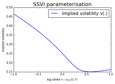 Figure 1
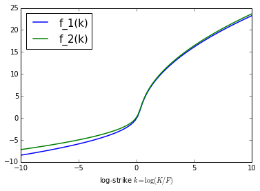 Figure 2
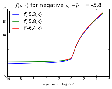 Figure 3
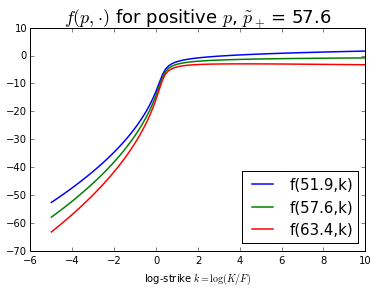 Figure 4
Peer Reviews
No public reviews on file for this paper yet. If you reviewed it on a platform where reviews are public (OpenReview, ICLR, NeurIPS, ICML), you can paste yours below so the community can read it here.
Videos
No videos yet. Explain this paper in a talk, walkthrough, or lecture? Add one.
Taxonomy
TopicsStochastic processes and financial applications · Financial Risk and Volatility Modeling · Stochastic processes and statistical mechanics
Moment generating functions and Normalized implied volatilities: unification and extension via Fukasawa’s pricing formula
Stefano De Marco111Ecole Polytechnique, CMAP, Université Paris-Saclay, France. [email protected], Claude Martini222Zeliade Systems, 56 rue Jean-Jacques Rousseau, Paris, France. [email protected]
We thank Masaaki Fukasawa and Jim Gatheral for stimulating discussions. We are much indebted with M. Fukasawa for raising our interest in this topic and for profound insights.
This PDF was obtained from an export from www.zanadu.ioZanadu.
1 Introduction
We consider an asset price at some fixed date . We denote the pricing (T-forward) measure, so that the price of a call option with maturity and strike is given by , where denotes the current price of the zero-coupon bond with maturity . We work with dimensionless quantities: we denote the forward log-strike, where denotes the forward price for maturity , and the dimensionless (or “total”) implied volatility. Recall that is defined for all by the equation \mathrm{Call_{BS}}(k,v(k))=\mathbb{E}\bigl{[}\bigl{(}\frac{S_{T}}{F}-e^{k}\bigl{)}^{+}\bigr{]}, where , is the standard normal cdf, and .
It is well-known that any (or convex) payoff with linear growth can be statically replicated with a strip of call and put options, so that its price can be written via Carr–Madan’s formula , where and denote put and call prices for the maturity , see e.g. [7, Eq (11.1)]. On the other hand, if the law of under is absolutely continuous with respect to the Lebesgue measure on , using the well-known Breeden-Litzenberger relations, one can write
[TABLE]
Applying the chain rule to the rightmost integrand in (1) leads to an integral formula containing Black-Scholes Greeks with respect to strike and volatility, and the derivatives of the implied volatility smile up to order two. A stream of literature [12, 7, 6, 2] studies the possibility of re-expressing Equation (1) in such a way that the derivatives of the implied volatility do not appear any more on the right hand side. This is a relevant feature in practice, because observed market data is (in any case) discrete. Such investigations required the introduction of the concept of normalizing transformation of the implied volatility smile, introduced by Chriss and Morokoff [3] and Matytsin [12] and formalized in the seminal work of Fukasawa [6], that we recall below.
One of the most important examples in this field is the following formula for the implied variance of the log contract333which coincides with the fair strike of the Variance Swap, under the assumption that follows a diffusion process. When and is the S&P500 stock index, the left hand side of (2) defines the (theoretical value) of at . , see Chriss and Morokoff [3] or Gatheral [7]:
[TABLE]
In (2), is the standard normal density, and is the inverse of the function (called second normalizing transformation)
[TABLE]
Similarly, the first normalizing transformation (used later on) is given by . Apart from its appealing compactness, the formula (2) is amenable for numerical approximations, notably in view of the use of Gauss-Hermite quadrature – see the discussions in [6, Remark 4.9] and Bergomi [2, p. 143]. Other examples of similar formulas include: other derivatives such as the contract (related to the Gamma Swap, see again [6] and Section 3 of this paper), and a formula for the characteristic function of due to Matytsin [12], see below. The important property that the map is actually invertible for any arbitrage-free implied volatility , implicitly assumed in the aforementioned works, was first proven by Fukasawa [6].
Matytsin’s formula for characteristic functions and Bergomi’s formula for .
Denote . Assuming that is differentiable, Matytsin [12] gives the following formula for the characteristic function of
[TABLE]
The proof of (3) is (only) sketched in Matytsin’s slides. Building on this work, Bergomi [2, Section 4.3.1] derives a formula for the moments of of order :
[TABLE]
where the “-normalized” implied volatility is defined in the following way: consider the convex interpolation
[TABLE]
of the two normalizing transformations and . We know from Fukasawa [6] that the two maps and are strictly increasing from to : therefore, so is , for every . Let bow be the inverse of on : is defined by
[TABLE]
(hence, with reference to Fukasawa’s notation, we have , ). Note we have the following nice interpretation of (4): in the Black-Scholes model, where is a geometric Brownian motion with constant volatility parameter , one has \mathbb{E}\bigl{[}\bigl{(}\frac{S_{T}}{F}\bigr{)}^{p}\bigr{]}=e^{\frac{1}{2}p(p-1)v^{2}}=\int_{\mathbb{R}}e^{\frac{1}{2}p(p-1)v^{2}}\phi(z)dz. Therefore, we can see Equation (4) as an extension of the pricing formula for power payoffs, from the Black-Scholes world to models with non-constant implied volatility.
The formulas (3) and (4) are the starting point of this work. As mentioned above, Bergomi [2] derives (4) from (3). Here, we will follow a different route: our starting point is the work of Fukasawa. We first extend the formula for expectations of functions of with polynomial growth given in [6, Theorem 4.6] to exponential functions – carrying out in details the plan addressed in [6, Remark 4.8]. This provides a formula for the generalized characteristic function on its analyticity domain, written directly in terms of the implied volatility smile. Matytsin’s (3) and Bergomi’s (4) formulas are embedded in this representation as special cases (along with a dual version of the first, and an extension to the complex plane of the second). By taking real values of , this formula allows to numerically evaluate the (finite) risk-neutral moments of the underlying asset price from the market smile – therefore identifying model-free quantities that can be used as targets in the calibration of a parametric model.
As addressed in [6, Remark 4.8], it is natural, when evaluating expectations of the form \mathbb{E}\bigl{[}\bigl{(}\frac{S_{T}}{F}\bigr{)}^{p}\bigr{]}, to exploit Lee’s moment formulas [10] relating the critical moments of to the asymptotic slopes of the implied volatility for large and small strikes. We stress that our approach here goes the other way round: we prove an integral representation for \mathbb{E}\bigl{[}\bigl{(}\frac{S_{T}}{F}\bigr{)}^{p}\bigr{]} without making use of Lee’s result. Then, as a by-product, we can deduce sharp bounds on the exponents that appear in the moment formulas.
The example of the SSVI parameterisation. Gatheral and Jacquier [8] propose the following parameterisation for total implied variance (the square of the dimensionless implied volatility ):
[TABLE]
where , and . The RHS of (6) provides a parameterisation of the whole implied variance surface, for every log-strike and every maturity . In the present setting, we are interested in parameterisations of a single arbitrage-free smile for a fixed maturity : for simplicity, we will therefore drop the index from the notation, and denote and . Important no-arbitrage properties of the SSVI model will be recalled in Section 7.
2 Extension of Fukasawa’s pricing formula
Our standing assumptions on the implied volatility are the following:
Assumption 2.1**.**
- (i)
* is twice differentiable on and for all .* 2. (ii)
**
Denote the law of under . It is classical that the second differentiability of is equivalent to the existence of a density with respect to Lebesgue measure for the restriction of to . Moreover, the strict positivity of is equivalent to the two conditions and , see [13]. In its turn, Assumption 2.1 (ii) is equivalent to . (In general, we have , see [14], [5].)
Remark 2.2**.**
Recall that for every from the arithmetic mean-geometric mean inequality, therefore we always have . Analogously, for every , hence . The limit of as is related to the arbitrage freeness of : indeed, is equivalent to the no-arbitrage condition . Therefore. always maps onto . Assumption 2.1 (ii) ensures that we have , so that is surjective, too.
Fukasawa [6] proves the following result:
Theorem 2.3** (Theorem 4.6 in [6]).**
Let be an absolutely continuous function with derivative of polynomial growth, and assume that there exists such that . Then,
[TABLE]
Analogously, if there exists such that , then \mathbb{E}\left[\frac{S_{T}}{F}\Psi\left(\log\frac{S_{T}}{F}\right)\right]=\int_{-\infty}^{+\infty}\bigl{[}\Psi(g_{1}(z))+\Psi^{\prime}(g_{1}(z))-\Psi^{\prime}(g_{2}(z))e^{g_{2}(z)}\bigr{]}\phi(z)dz.
Equation (7) can be proven starting from (1) and then applying judicious integration by parts, and change of variables by means of the transformations and . Important steps in this proof, see [6], are (i) ensuring the integrability of the involved integrands, and (ii) checking that the boundary terms arising from integration by parts do give zero contribution (point (ii) amounts to showing that , see Lemma A.2 in the Appendix).
Setting in (7) would give us a formula for the moment of of order . Unless , such a function falls outside the class of functions covered by Theorem 2.3. We therefore proceed to extend Theorem 2.3 to this setting.
2.1 Functions with exponential
growth
Define the two functions
[TABLE]
and set if . It is easy to see that and , for all . The expressions above of the functions arise from certain integrability conditions of the integrand in (7) when , as we will explain more precisely below. Now, if we denote
[TABLE]
the right, resp. left, critical exponent of (note we define to be positive), then Roger Lee’s moment formula [10] states that:
[TABLE]
where
[TABLE]
As pointed out in the introduction, in the present work we do not make use of Lee’s result in order to extend Equation (7) to functions with exponential growth. In other words, we do not use the information or at any point.
Example 2.4**.**
For the SSVI parameterisation (6) we have
[TABLE]
As we will recall in section 7.1 below, a necessary condition for no arbitrage is , so that .
The quantitative link between (7) and (10) can be highlighted with some simple calculations: assume (only within this paragraph) that the first equation in (11) hold as a limit, and that . Then, from the definition of and ,
[TABLE]
Using the definition of the maps , it is easy to see that Eq (13) implies a quadratic behavior of and for large :
[TABLE]
Now, a formal application of (7) to leads to \mathbb{E}\bigl{[}\bigl{(}\frac{S_{T}}{F}\bigr{)}^{p}\bigr{]}=\int_{\mathbb{R}}\bigl{[}pe^{(p-1)g_{1}(z)}+(1-p)e^{pg_{2}(z)}\bigr{]}\phi(z)dz. Applying (14), a straightforward calculation yields
[TABLE]
The last estimates above show that is precisely the threshold between Gaussian integrability (when ) or, on the contrary, exploding behavior (when ) for the two functions and inside the integral (for positive ). The analogous argument allows to show that is the threshold between integrability and explosion of the integrand for negative . Some more work (which we perform in the proof of Theorem 2.7 below) is required to study the asymptotic behavior of the linear combination , and to deal with the remaining cases .
Definition 2.5**.**
We say that a function has exponential growth of order for some if the function is bounded.
Lemma 2.6**.**
Let such that
[TABLE]
where are defined in (8), and let be an absolutely continuous function such that and have exponential growth of order . Then, the functions
[TABLE]
are integrable on .
With a view on Lemma 2.6, note that the bound for (resp. for ) entails
[TABLE]
Since is eventually positive for large , the estimate (16) follows from (resp. for sufficiently small). Therefore, for every ,
[TABLE]
For every function with exponential growth of order , we have and . Consequently, the estimates in (17) show that the functions in (15) are always integrable for every and for every arbitrage-free smile (regardless of the values of ).
Theorem 2.7**.**
Let such that
[TABLE]
where are defined in (8) and in (11). Let be an absolutely continuous function such that and have exponential growth of order . Then,
[TABLE]
In particular, for all ,
[TABLE]
The proofs of Lemma 2.6 and Theorem 2.7 are given in Appendix A. The formula (20) for the moments of was mentioned in the introduction of [6], the extension of Thm 2.3 to functions with exponential growth being implicitly assumed therein.
We stress once again that our proof of Theorem 2.7 does not make use of Lee’s result [10]. As an immediate consequence of Theorem 2.7, we have the following bounds:
Corollary 2.8**.**
Let be defined by (8) and by (9). Then
[TABLE]
In particular, if and if .
Proof.
From Equation (20), we have for all . The claim then follows from the definition of and . ∎
Remark 2.9**.**
Our proof of Theorem 2.7 in Appendix A is obtained essentially by rerunning the explicit computations linking the LHS to the RHS in (19), showing that i) all the required integrability conditions are met, and ii) that integration by parts produce zero boundary terms. Another approach to the proof of (20) would go as follows: apply Fukasawa’s result (Theorem 2.3 above) to the functions , which have polynomial growth for every . Under the assumption , this yields \mathbb{E}[\Psi_{n}(X_{T})]=\int\bigl{[}\bigl{(}1+\frac{pg_{2}(z)}{n}\bigr{)}^{n}-p\bigl{(}1+\frac{pg_{2}(z)}{n}\bigr{)}^{n-1}+p\bigl{(}1+\frac{pg_{1}(z)}{n}\bigr{)}^{n-1}e^{-g_{1}(z)}\bigr{]}\phi(z)dz. By monotone convergence, the left hand side converges to for every . On the other hand, if the RHS converges to \int\bigl{[}pe^{(p-1)g_{1}(z)}+(1-p)e^{pg_{2}(z)}\bigr{]}\phi(z)dz by dominated convergence, thanks to Lemma 2.6. This argument proves Eq (20) for every such that ; some additional work then allows to prove the inequalities and (we use a similar argument in Appendix A), and the claimed result then follows for every in (18).
Following our (alternative) proof in Appendix A, we get rid of the limitation (or ) from Theorem 4.6 in [6]. This is related to the growth condition we consider on the function , which is “one-sided”: while, in Definition 2.5, is allowed to grow faster than a polynome for large arguments (if, say, ), on the other side has to go to zero for (as opposed to the polynomial growth condition in [6, Theorem 4.6], which allows to diverge on both sides).
Remark 2.10** **(About the proof of the converse inequalities for
and , using Theorem 2.7).
The function p\mapsto M(p)=\mathbb{E}\bigl{[}\bigl{(}\frac{S_{T}}{F}\bigr{)}^{p}\bigr{]} in Theorem 2.7 is the bilateral Laplace transform of a probability measure on (the law of ). Its positive and negative abscissas of convergence are, respectively, and defined in (9); moreover, has a unique holomorphic extension to the strip .
Assume : then, would be a holomorphic extension of the function , defined on , to . If we prove that this is not possible – that is, that cannot be extended analytically to any neighbourhood of – then we would have shown by contradiction that , therefore by Lemma 2.8. The symmetric argument of course applies to the inequality .
It is not difficult to prove, using similar arguments to the proof of Theorem 2.7, that the function (as defined by the left hand side of Eq (20)) is infinite for every if the implied volatility slope has a limit. More precisely, we can show:
- •
Assume that exists. Then, for every .
- •
Assume that exists. Then, for every .
*Note we are not (yet) showing here that does not admit a holomorphic extension to a neighbourhood of or . Let us just observe, for the moment, that the proof of this statement (that we leave for future work) might not be so straightforward. We can see as a linear combination of Laplace transforms of positive functions, . Since the coefficients and have opposite signs as soon as or , even if each Laplace transform cannot be extended analytically above (or below ), the behavior of their linear combination is more subtle to study. *
2.2 Extension to the complex plane
We can extend Theorem 2.7 to the following
Proposition 2.11**.**
The identity
[TABLE]
holds for all with .
Proof.
By Lemma 2.6, Equation (20) defines a holomorphic function on . In its turn, the function is holomorphic on . From Theorem 2.7, these two functions coincide on the interval , therefore they also coincide on . ∎
3 Duality for normalized implied volatilities
In this section, we investigate the consequences of put-call duality on the normalized implied volatilities , .
Let us briefly recall the put-call duality relation and its (standard) consequences for the implied volatility . Let us drop the index from notation, and write , where is a positive random variable with . Consider the change of measure . Set (note that ). We look for a relation between the implied volatilities of under and under . We have:
[TABLE]
Consider now the particular case of the Black-Scholes model where , where is the Doleans–Dade exponential, a Brownian motion and . Then, the distributions of under and under are the same. The equality between the outermost terms in the above chain of equalities rewrites:
[TABLE]
where (resp. ) denotes the price of the Black-Scholes call (resp. put) option with strike , forward value , and total implied volatility . Now, by the definition of the implied volatility we have and \mathbb{E}^{\mathbb{P}}\bigl{[}\bigl{(}\frac{F^{2}}{K}-S\bigr{)}^{+}\bigr{]}=P_{\mathrm{BS}}\bigl{(}\frac{F^{2}}{K},F,V\bigl{(}\frac{F^{2}}{K}\bigr{)}\bigr{)}. Applying (22) and (23), we get
[TABLE]
therefore \hat{V}(K)=V\bigl{(}\frac{F^{2}}{K}\bigr{)} for all . In terms of (resp. ), this reads
[TABLE]
We immediately have the following:
Lemma 3.1**.**
Let (resp. ) the first and second normalizing transformations associated to (resp. to ). Let , , and the inverse function of for (and likewise for and ). Then
[TABLE]
and
[TABLE]
In particular
[TABLE]
Proof.
The first bullet point follows immediately from (24) and the definition of the normalizing transformations: , and the claim follows. The second bullet point is a direct consequence of the first: rewrites , therefore . Equations (25) are special cases for and (recall that, with our notation, ). ∎
Proposition 3.2**.**
Let (resp. ) the -normalized implied volatility associated to (resp. ), as defined in (5). Then,
[TABLE]
In particular, and .
Proof.
Applying (24) and Lemma 3.1, we have . The last claim is a special case of (26), recalling that, with our notation, , . ∎
As an example, using formula (2) for the price of the log contract and Proposition 3.2, we obtain the following formula for the implied variance of the contract (corresponding to the de-annualized fair strike of the Gamma Variance Swap in a diffusion model):
[TABLE]
which is formula (1.2) in [6].
Remark 3.3**.**
As another application of the duality (25), we can deduce the invertibility of the first normalizing transformation from the invertibility of the second (or vice-versa). Precisely, we have the following: the map (resp. ) is strictly increasing for every arbitrage-free smile if and only if (resp. ) is such.
Remark 3.4**.**
The formula (20) for the moments of is invariant under the duality transformations , and . This is consistent with Lemma 3.1: indeed, note that
[TABLE]
Equation (20) yields, for every ,
[TABLE]
Applying the identities and in Lemma 3.1, it is immediate to check that the rightmost term in the above equation coincides with , therefore with as expected.
4 Alternative representations and Matytsin’s
formula
The formula (21) is written in terms of the two normalizing transformations and . We can recast it into an equivalent formula containing only the normalized implied volatility and its derivative (or yet, a dual formula in terms of ). The original formula (3) of Matytsin [12] is a special case of this representation.
Recall the definition and the following relation between and : by definition, we have , which yields
[TABLE]
Analogously,
[TABLE]
Proposition 4.1**.**
For every with ,
[TABLE]
Proof.
Starting from (21), we have
[TABLE]
where we used the identity . By definition of and , we have , which yields
[TABLE]
for . Plugging (31) into (30), we obtain
[TABLE]
from which the claim follows using (27). ∎
We have the following dual formula:
Proposition 4.2**.**
For every with ,
[TABLE]
Proof.
Follows by mimicking the proof of Prop 4.1, now applying the identities and (28). ∎
Remark 4.3**.**
The two formulas (29) and (32) are the dual of each other: that is, they are related via the transformations , . In fact, instead of proving Equation (32), we could infer it from (29), applying the duality results of Section 3. This goes as follows: use Equation (29) to compute \hat{M}(1-p)=\mathbb{E}^{\hat{\mathbb{P}}}\bigl{[}\bigl{(}\frac{\hat{S}_{T}}{F}\bigr{)}^{1-p}\bigr{]} in terms of . Applying the identities from Remark 3.4 and from Proposition 3.2, we obtain (32).
Corollary 4.4**.**
Taking for in (29), we obtain Matytsin’s formula [12]
[TABLE]
Taking for in (32), we obtain the dual formula
[TABLE]
As an exercise, we can reobtain Chriss and Morokoff’s formula [3] for by computing .
5 Extension of Bergomi’s formula to ,
In this section, we follow Bergomi’s idea [2] of interpolating the two transformations and . When is real-valued, this procedure allows to turn Equation (20) into (yet) another formula for , now written in terms of the -normalized implied volatility : the result is the compact and elegant formula (4) (which is also self-dual, cf. Remark 5.3 below). Starting from Proposition 2.11, we can now extend Bergomi’s formula to the complex plane.
Note that we can extend the definition of the function to in the obvious way, setting for every . This gives
[TABLE]
so that the map is one-to-one from onto the following curve in the complex plane:
[TABLE]
Consequently, for every with , we can define the inverse of from to by
[TABLE]
where, with a slight abuse of notation, we still denote the support of the curve. Finally, we can extend the definition of the -normalized implied volatility to complex :
[TABLE]
so that .
Theorem 5.1**.**
For every in the strip ,
[TABLE]
where and the curve is defined in (34).
Proof.
In the proof of Prop. 4.1, we have shown that . Therefore, using (33),
[TABLE]
where we have used the identity in the second line. Now, Eqs (27) and (28) are easily generalized to , which yields . Plugging this last identity inside (36), after some straightforward simplifications, we obtain (35). ∎
Remark 5.2**.**
Theorem 5.1 shows that Matytsin’s formula (3) and Bergomi’s (4) can be written as line integrals of the same function on different curves in the complex plane. Bergomi’s formula is obtained setting in (35): in this case, . Matytsin’s formula is obtained (again) setting in (35): in this case, (recall that corresponds to Fukasawa’s ).
Re-injecting the expression of , formula (35) can of course be written as the following (less compact) integral on the real-line
[TABLE]
which does not require the notion of transformation and volatility for complex-valued and .
Remark 5.3**.**
Just as the Equation (20) we started from, the formulas (35) and (37) are also self-dual: they are invariant under the transformations .
The restriction in Theorem 5.1 is imposed by the invertibility requirement for the interpolated transformation . In the next section, we investigate the invertibility of this map for values of that lie outside . We will see that (apart from the trivial Black-Scholes case) there are examples of smiles for which the map remains strictly monotone on some interval (and possibly on the whole ) for all or all .
6 The invertibility of
We know (from the result of Fukasawa [6]) that the interpolated transformation associated to any arbitrage-free implied volatility is strictly increasing if is in . On the other hand, in the Black-Scholes model with constant volatility parameter , the map k\mapsto f(p,k)=\frac{k}{\sigma\sqrt{T}}+\Bigl{(}\frac{1}{2}-p\Bigr{)}\sigma\sqrt{T} is (linear, hence) trivially invertible, for every . It is natural, then, to wonder what happens in general – that is, if there are other cases where is invertible when lies outside , and if so, whether one can characterize (in terms of the smile, or of the underlying distribution) the values of for which this happens.
6.1 is surjective for every in an interval
larger than
A reasonable guess would seem to conjecture that is invertible when is between the critical exponents, . The following proposition shows that is actually surjective for every in an interval that is larger than .
Proposition 6.1**.**
Recall that . Define
[TABLE]
where if . We have resp. , where the inequalities are strict if , resp. . Moreover
if , then .
- -
if , then .
In particular, if , the map is surjective on .
Proof.
The comparison between and (resp. and ) is immediate to check. Let us, then, prove the statements about the limits of .
Assume . First note that, if , we have as . Then, assume . If , there is nothing more to prove, because in this case . If , then using estimate (47), for every we have
[TABLE]
for some . The condition entails . Therefore, when is sufficiently close to , the coefficient in front of in (38) is positive, so that .
The symmetric argument holds when . Let us provide the details: First, if , then as . Then, assume . Once again, if , there is nothing more to prove, because in this case . If , then using estimate (52), for every we have
[TABLE]
for some . The condition entails . Therefore, when is sufficiently close to , the coefficient in front of is negative, so that . ∎
6.2 Some results on the monotonicity of
In this section we show that there exist (non trivial, and practically interesting) situations where the map is strictly monotone for values of that lie outside . We start with the following lemma.
Lemma 6.2**.**
On the set , we have , for every .
On the set , we have , for every .
The first case in Lemma 6.2 is relevant in particular in Equity markets, where smiles on stock indices are often monotonically decreasing on the observed interval of strikes (in particular for larger maturities).
Proof.
We first focus on the case . Using the identities
[TABLE]
we have
[TABLE]
We know from [6, Lemma 2.6] that for all . The conclusion follows.
The case follows from duality (Section 3): by Lemma 3.1, we have , therefore , where is larger than . In the first part of the proof, we have shown that on . Since from Eq (24), we have , and the second claim follows. ∎
Proposition 6.3**.**
* If the implied volatility is decreasing, then and the function is invertible from to , for all .*
* If the implied volatility is increasing, then and the function is invertible from to , for all .*
Proposition 6.3 allows us to extend the definition of the normalized implied volatility in Eq (5) to every if we start from a decreasing smile (resp. to every if we start from an increasing smile). As an application:
Corollary 6.4**.**
The extended Bergomi’s formula (5.1) holds for all in case i) of Proposition 6.3, resp. in case ii).
Proof of Proposition 6.3.
Let us consider the first case ( is increasing). We have to prove the statement for , for we already know that is invertible for . It follows from Lemma 6.2 that is strictly monotone for every . Since, by assumption, has a finite limit for , we have , therefore . It then follows from Proposition 6.1 that is surjective on for every , and the claim is proved. The second case ( is decreasing) is proven in the same way, using Lemma 6.2 and Proposition 6.1 with . ∎
A class of smiles for which is not invertible when . We now exhibit a large class of implied volatilities (with finite critical moments, hence finite coefficients ) for which the function fails to be both monotone and surjective when is outside the interval . Consider the following assumption
[TABLE]
By de L’Hopital’s rule, implies as , therefore we have (11). Note that the SSVI parameterisation (6) with satisfies assumption (recall Eq (12)).
Using the definition of , it is straightforward to check that assumption (H) implies
[TABLE]
The limits of for are then easily assessed: the case is already considered in Proposition 6.1; if lies outside the closure of this interval, then both limits have the same sign:
[TABLE]
In particular we see that, being continuous, the map cannot be surjective on when .
Proposition 6.5**.**
Assume . Then, if or , the map is neither monotone, nor surjective.
More precisely: If (resp. ), there exist and such that is strictly increasing (resp. decreasing) on and strictly decreasing (resp. increasing) on .
A numerical example of the situation described in Proposition 6.5 will be given in the next section – see Figure 2.
Proof of Proposition 6.5.
The statement about the surjectivity of has already been proven above (recall (40)); we prove that is not monotone.
Let us first consider the case . The condition as implies that is negative on the half-line , for some . It follows from Lemma 6.2 that is strictly increasing on .
Using the first equation in (39), together with the identity , we have
[TABLE]
It follows from assumption that
[TABLE]
therefore
[TABLE]
It is immediate to see that . Consequently, if , it follows from (41) that is negative for large enough, and the claim on the intervals of monotonicity of is proven.
We can now deduce the claim in the case from duality: consider the dual implied volatility defined in Section 3. It follows from (24) and assumption (H) that as and as , so that (the duality transformation exchanges the right and left slopes of the smile). Denote the coefficient associated to , that is: . We know from Lemma 3.1 that . Since , then . In the first part of the proof, we have proven that is strictly increasing on the half-line for some , and strictly decreasing on for some , therefore the claim on the monotonicity of follows. ∎
In view of Propositions 6.1, 6.3 and 6.5, it seems reasonable to conjecture that the map is invertible if , and only if . Leaving the proof of this statement for future work, we numerically check this fact on an arbitrage-free SSVI parameterisation in the next section.
7 The case of the SSVI parameterisation
Recall the SSVI parameterisation (6), where, for fixed ,
[TABLE]
7.1 No-arbitrage conditions
Theorem 4.2 in [8] proves that the implied variance is free of arbitrage (for the given maturity ) if the following conditions are satisfied:
Condition 7.1**.**
[TABLE]
Moreover, [8, Lemma 4.2] shows that the condition is necessary. The inequality 2) in Condition 7.1 is sufficient, but not necessary.
We cross-check below that, under Condition 7.1, our standing Assumptions 2.1 (i) and (ii) on are (as one could expect) satisfied. We also further discuss the limiting case .
7.2 The limiting case and
checking Assumption 2.1 (ii) on
We show that the case and is not arbitrage-free. Therefore, if , Condition 7.1(1) (with strict inequality) is also necessary. When , we show that the case is ruled out by our Assumption 2.1 (ii) of zero mass at .
Assume . We separate the two cases and : assume first that . It is easy to see that . Then we can compute, for :
[TABLE]
The limit above contradicts the following property from [10, Lemma 3.1]: if is an arbitrage-free smile, there exists such that for every .444This property was subsequently improved to by Rogers and Tehranchi [13].
Now assume . The analogous computation for negative gives
[TABLE]
In general, a positive value of is not in contradiction with no-arbitrage: indeed, we know from [5, Propositions 2.4 and 2.5] that an arbitrage-free implied volatility satisfies
[TABLE]
where the right hand side is worth if (see also [4, Thm 3.6]). As discussed in the Introduction, our Assumption 2.1 (ii) on the coefficient is equivalent to , therefore as . Consequently, v^{2}(k)-2|k|=\bigl{(}v(k)-\sqrt{2|k|}\bigr{)}\bigl{(}v(k)+\sqrt{2|k|}\bigr{)} tends to as well, and the case and is ruled out by Assumption 2.1 (ii).
Finally, a slight modification of the computation above allows to see that, if , we have as with a=\frac{1}{2}\bigl{(}4-\theta\varphi(1+|\rho|)\bigr{)}>0, therefore Assumption 2.1 (ii) is satisfied when Condition 7.1(1) is in force.
7.3 Checking Assumption 2.1 (i) on
Denote . We can compute
[TABLE]
Note that the second equation shows that is a convex function. If , is identically equal to (so that this case corresponds to Black-Scholes implied volatility). Let us assume, then, . From the first equation in (43), if and only if . At this point, we have
[TABLE]
A straightforward computation shows that the function of in the RHS above is strictly positive, for any . This guarantees that .
Moreover, the argument of the square-root function in (6) being lower bounded by , we have (actually, ). Since , we also have that is . Overall, Assumption 2.1 (i) is also satisfied.
7.4 Numerical tests
It is immediate to check that the set of parameters
[TABLE]
satisfies Condition (7.1). Figure 1 shows the resulting SSVI implied volatility smile and the two corresponding transformations and , on a large interval .
Recall that . In Figure 2, we compute the values of the coefficients in Proposition 6.1, and plot the function for different values of . As predicted by Proposition 6.5, one can see (and we did check on the numerical values) that is not increasing anymore for large (resp. small) when is larger than (resp. is smaller than ). On the contrary, does appear to be strictly increasing (at least on the considered interval of log-strikes) for within the interval .
8 Recovering the Black-Scholes formula
Having derived formulas for the extended characteristic function of the log-price, prices of European options on can (also) be recovered with standard transform-based methods. As a consistency check, we show that the formula for a put option (the Black-Scholes formula) can be restored from Theorem 2.7. We assume and for simplicity. We apply the following inversion theorem (see e.g. [11]):
Theorem 8.1**.**
Denote the characteristic function of the log-price. Then, for every , the price of a put option with strike and maturity is given by:
[TABLE]
where
[TABLE]
Applying Theorem 8.1 and Proposition 2.11 we get, choosing and using :
[TABLE]
Using Fubini’s Theorem,
[TABLE]
or yet, after simplification:
[TABLE]
Set . Then
[TABLE]
where
[TABLE]
We show now:
Lemma 8.2**.**
If and , then .
If and , then .
If and , then .
If and , then .
Proof.
Consider first the case , and the rectangle defined by the real coordinates and and the imaginary coordinates wih positive and . By Cauchy residue formula, the integral of the function over this (clockwise) rectangle contour is equal to [math] if , or to the residue at the pole [math], which is , times because we go clockwise, if the pole [math] is inside the rectangle, i.e. if . Now take to : since is positive, the integral on the right segment goes to zero, and the integral on the bottom and top segments are absolutely convergent. By Lebesgue dominated convergence theorem, those integrals go to zero as goes to infinity. Since the remaining integral is exactly , we have proven the last two statements. The proof of the case is exactly the same, working with the real coordinates and instead, and running anticlockwise on the rectangle contour. ∎
Since , the contribution of the first term on the RHS of (46) is given by the case , so that
[TABLE]
For the second term, we are in the case , so that the contribution is
[TABLE]
Summing up, we have recovered the Black-Scholes formula for the put option:
[TABLE]
Appendix A Appendix
Proof of Lemma
We focus on the case . As explained above, the statement of the Lemma is true for every . Therefore, we can limit ourselves to , and assume .
By definition of , we have the following: for every , there exists such that for all . We claim that this implies
[TABLE]
It follows from (47) that
[TABLE]
which entails . On the other hand, using , we obtain for all , therefore for large enough. For such , we have
[TABLE]
and
[TABLE]
Recall that for every . Since by assumption, taking sufficiently close to , we have , too. Therefore, using the last two estimates above, we obtain that the functions in (15) are integrable at . Using the fact that as and , we obtain that the functions in (15) are also integrable at .
The case is proven analogously.
Proof of (47) : We proceed along the lines of [5, Lemma 2.6] (note that we are referring here to an ArXiv preprint: this lemma was not reported in the published version of the article). For every and , we have
[TABLE]
where the last inequality holds because the arithmetic mean is larger than the geometric mean. Estimate (47) then follows by choosing (which in fact provides the optimal lower bound in (48)). ∎
A.1 Proof of Theorem 2.7
We first prove a weaker version of Theorem 2.7:
Proposition A.1**.**
Assume
[TABLE]
Then, Equation (19) holds for every absolutely continuous function such that and have exponential growth of order .
In order to prove Proposition A.1, we need the following intermediate result.
Lemma A.2**.**
Assume that satisfies (49), and let be a function with exponential growth of order . Then, the function is integrable on , and satisfies .
In the proof of Lemma A.2, we will make use of the identity
[TABLE]
which can easily be derived from Black-Scholes formula and the definition of , \mathrm{Call_{BS}}(k,v(k))=\mathbb{E}\bigl{[}\bigl{(}\frac{S_{T}}{F}-e^{k}\bigr{)}^{+}\bigr{]}. Using the identity , we also have the equivalent formulation
[TABLE]
Remark A.3**.**
It follows from expression (50) that , in particular this quantity is bounded, so that the condition holds for functions going to zero at infinity.
Proof of Lemma
A.2.
In what follows, denotes a positive constant that can change from line to line, but does not depend on nor on any other parameter. Let be of exponential growth of order .
Using the boundedness of from Eq (50), we have . Therefore, if , and this function is integrable in a neighborhood of . On the other hand, using again Eq (50), the bound for , and the bound on Mill’s ratio for , we have
[TABLE]
For the second term, note that entails as , for every (for a proof of this fact, see [9, Lemma 4.4]). It follows that, if , and that this function is integrable in a neighborhood of . Overall, the conclusion of Lemma A.2 is true for every and every function of exponential growth of order (regardless of the values of ).
According to the first bullet point, we can limit ourselves to . Assume that is in the interval (49). It follows from Eq (50) and estimate (47) that, for every ,
[TABLE]
By assumption, . Choosing sufficiently close to , we have , too (in the particular case , we can make arbitrarily small by taking small enough).
For the second term in the last line, note that the right critical moment satisfies , see again [9, Lemma 4.4]. Therefore, for every , as . Taking , we can conclude that and that is integrable in a neighborhood of .
The analogous argument holds for the left side behavior of : let us provide the details for completeness. From the first bullet point, we can assume . By definition, for every , there exists such that for all . It follows that
[TABLE]
In order to prove (52), note that for every and
[TABLE]
from which we obtain by choosing . Then, (52) follows from .
Consequently, if is in the interval (49), using Eq (51) and estimate (52), for every we have
[TABLE]
By assumption, . Choosing sufficiently close to , we have , too. For the second term in the last line, we use the property [9, Lemma 4.4], which entails for every . Taking , we conclude that and that is integrable at .
Putting the three bullet points together, we have shown that Lemma A.2 holds for any value of . ∎
Proof of Proposition A.1
We follow the lines of [6, Theorems 4.6 and 4.4]. Denote the LHS of (19): . Using the identity , we have
[TABLE]
Integrating by parts, applying Lemma A.2 and using the identity , we get
[TABLE]
It follows from Eqs (53) and (54) that . Now recall that, under the assumption that is twice differentiable, the density function of at the point is given by
[TABLE]
where we have used the identities and, again, . Applying (55), we obtain
[TABLE]
therefore Equation (19) is proved under condition (49) on . ∎
We finally have to strengthen Proposition A.1 into Theorem 2.7. If we know that and , this is immediate. Recall anyhow that our intention here is not to make use of Lee’s result [10], therefore these bounds need to be proved.
The key ingredient will be the following result from the theory of Laplace transforms. Let such that a.e. Define and denote the abscissa of convergence of , where . Then, defines a holomorphic function on .
Lemma A.4** (Theorem 2.7.1 in [1]).**
Let such that a.e. Assume that . Then, cannot be extended to a holomorphic function on a neighbourhood of .
Lemma A.4 allows to prove the bounds we need in order to conclude.
Lemma A.5**.**
* and .*
Proof.
We focus on the first inequality, . Assume . We have , where is the density of (which exists under Assumption 2.1 (i) on the implied volatility ). From Proposition A.1, the identity
[TABLE]
holds on . By definition of , . On the other hand, is holomorphic on the half-plane , and is holomorphic on the strip by Lemma 2.6. In other words, the function is a holomorphic extension of to the strictly larger strip , contradicting Lemma A.4. The second inequality is proven analogously. ∎
As pointed out above, the proof of Theorem 2.7 is now immediate.
Proof of Theorem 2.7 Lemma A.5 implies and . Equation (19) then follows from Proposition A.1. Equation (20) is (19) for the function .
The reference list from the paper itself. Each links out to its DOI / PubMed record.
- 1[1] W. Arendt, C. Batty, M. Hieber, and F. Neubrander , Vector-valued Laplace Transforms and Cauchy Problems , Monograph in Mathematics 96, Springer Basel, second ed., 2011.
- 2[2] L. Bergomi , Stochastic Volatility Modeling , Chapman and Hall/CRC, 2016.
- 3[3] N. Chriss and W. Morokoff , Market risk for volatility and variance swaps , Risk, 1 (October 1999), pp. 609–641.
- 4[4] S. De Marco, C. Hillairet, and A. Jacquier , Shapes of implied volatility with positive mass at zero . Forthcoming in SIAM J. Financ. Math. https://arxiv.org/abs/1310.1020, 2013.
- 5[5] M. Fukasawa , Normalization for implied volatility . Preprint Ar Xiv, https://arxiv.org/abs/1008.5055, 2010.
- 6[6] , The normalizing transformation of the implied volatility smile , Mathematical Finance, 22 (2012), pp. 753–762.
- 7[7] J. Gatheral , The Volatility Surface: A Practitioner’s Guide , Wiley Finance, 2006.
- 8[8] J. Gatheral and A. Jacquier , Arbitrage-free svi volatility surfaces , Quantitative Finance, 14 (2014), pp. 59–71.