Alternative steady states in random ecological networks
Yael Fried, Nadav M. Shnerb, David A. Kessler

TL;DR
This paper investigates the number of stable, uninvadable states in large, random ecological networks, revealing exponential growth with species number under certain conditions and linking it to network clique structures.
Contribution
It introduces a model connecting stable states in ecological networks to maximum cliques in near-complete graphs, especially in the weak competition and high variance limit.
Findings
Number of stable states grows exponentially with species in symmetric networks.
Asymmetry in competition reduces the number of stable states to a constant order.
Numerical simulations support the applicability to continuous competition distributions.
Abstract
In many natural situations one observes a local system with many competing species which is coupled by weak immigration to a regional species pool. The dynamics of such a system is dominated by its stable and uninvadable (SU) states. When the competition matrix is random, the number of SUs depends on the average value of its entries and the variance. Here we consider the problem in the limit of weak competition and large variance. Using a yes/no interaction model, we show that the number of SUs corresponds to the number of maximum cliques in a network close to its fully connected limit. The number of SUs grows exponentially with the number of species in this limit, unless the network is completely asymmetric. In the asymmetric limit the number of SUs is . Numerical simulations suggest that these results are valid for models with continuous distribution of competition terms.
Click any figure to enlarge with its caption.
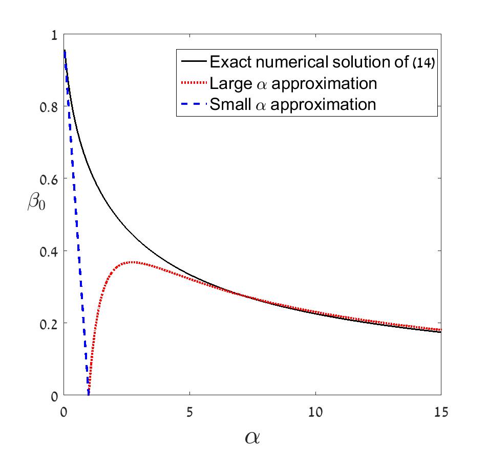 Figure 1
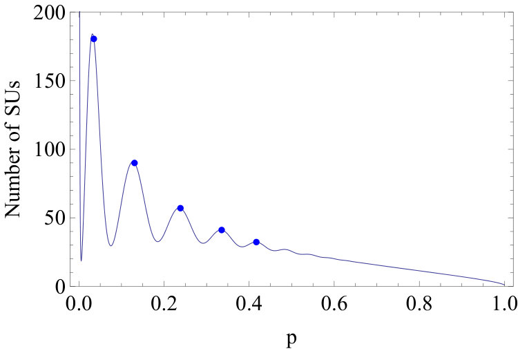 Figure 2
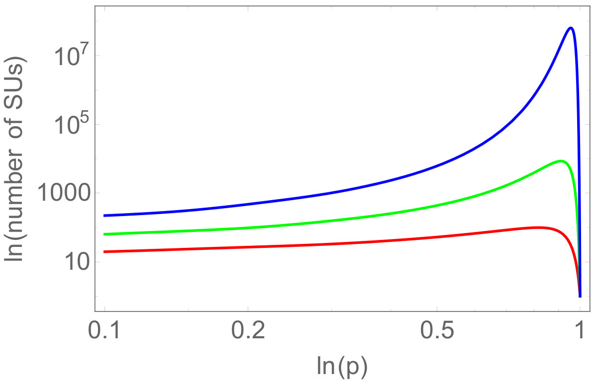 Figure 3
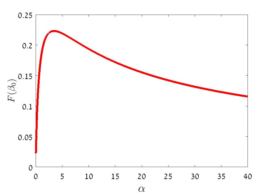 Figure 2
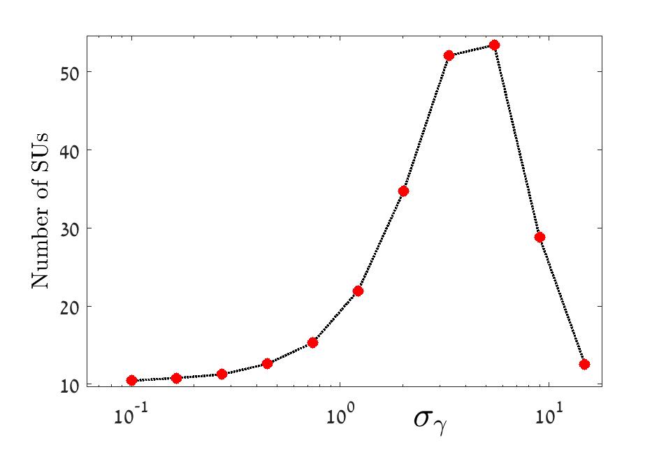 Figure 4
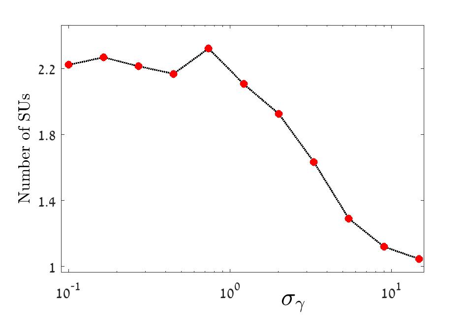 Figure 6
Peer Reviews
No public reviews on file for this paper yet. If you reviewed it on a platform where reviews are public (OpenReview, ICLR, NeurIPS, ICML), you can paste yours below so the community can read it here.
Videos
No videos yet. Explain this paper in a talk, walkthrough, or lecture? Add one.
Alternative steady states in random ecological networks
Yael Fried
Department of Physics, Bar-Ilan University, Ramat-Gan IL52900, Israel
Nadav M. Shnerb
Department of Physics, Bar-Ilan University, Ramat-Gan IL52900, Israel
David A. Kessler
Department of Physics, Bar-Ilan University, Ramat-Gan IL52900, Israel
Abstract
In many natural situations one observes a local system with many competing species which is coupled by weak immigration to a regional species pool. The dynamics of such a system is dominated by its stable and uninvadable (SU) states. When the competition matrix is random, the number of SUs depends on the average value of its entries and the variance. Here we consider the problem in the limit of weak competition and large variance. Using a yes/no interaction model, we show that the number of SUs corresponds to the number of maximum cliques in a network close to its fully connected limit. The number of SUs grows exponentially with the number of species in this limit, unless the network is completely asymmetric. In the asymmetric limit the number of SUs is . Numerical simulations suggest that these results are valid for models with continuous distribution of competition terms.
I Introduction
The richness of ecological communities poses a prolonged theoretical challenge. Focusing on guilds of many species competing for a common resource (and neglecting, for the moment, processes like predation or mutualism) the main problems are two. First, the competitive exclusion principle Gause (1934); Hardin (1960) suggests that the result of competition for a single limiting resource is the extinction of all except the fittest speices, and that in the presence of a few limiting resources the equilibrium number of species is smaller than or equal to the number of resources Tilman (1982). Second, even if the number of limiting resources is large, May May (1972) pointed out that if the niche overlap between species is substantial the chance of a system of species to admit a stable equilibrium decreases exponentially with . May’s result is based on the spectral properties of random stability matrices. Practically, it implies that to achieve a stable coexistence of more than 6-8 species one has to fine-tune the competition parameters in an unrealistic manner.
However, in many situations the (inter and intra) specific dynamics takes place on local patches, which are coupled by migration to each other or to a regional pool. Accordingly, many ecological models are focused on the dynamics of a local patch, putting aside the global stability problem. A mainland-island model MacArthur (1967); Losos and Ricklefs (2010) is the simplest scenario considered in this context: a set of local populations of different species are competing with each other and the island is exposed to weak migration from a static pool of species on the mainland. The structure of the community on the island reflects a balance between local extinctions and colonization by immigrants from the mainland. Extinctions may be either deterministic, due to the pressure that a species suffers from its competitors (or from the local environment), or stochastic, caused by the random nature of the birth-death process Kessler and Shnerb (2007); Ovaskainen and Meerson (2010) possibly superimposed on the effect of environmental variations Lande et al. (2003); Danino et al. (2016).
In a recent work Kessler and Shnerb (2015), Kessler and Shnerb suggested a classification of the qualitative features of the community on the island. Four different “phases” were identified.
- I.
Full coexistence: If the interspecific competition is weak (say, if different species use essentially different resources) any species in the mainland may invade the island and establish a finite population, so all species are present on the island. Local extinctions still occur but if the local populations in steady state are large, these events are rare and transient. Technically speaking, the deterministic (i.e., noise-free) model allows for a stable fixed point with all the species coexisting. 2. II.
Partial coexistence: As the competition among species grows, the species’ abundances decay as they feel more pressure from other species. Since the competition matrix is heterogenous, some species feel more pressure than others, and the deterministic model eventually allows for a stable fixed point for a finite subset containing of the species. The other species on the mainland cannot invade the island, i.e., their growth rate at low densities on the island is negative. 3. III.
Disordered: When the competition increases even further, *and the competition matrix is not symmetric *(meaning that species 1 may put a lot of pressure on species 2 but species 2 puts much less pressure on species 1, say), the system may not have an attractive fixed point at all or, even if it have one, its basin of attraction will be very narrow. In the presence of noise, the system fails to converge to an equilibrium state and instead it shows intermittent behavior with many long excursions that reflect high-dimensional chaotic/periodic trajectories. 4. IV.
Alternative steady states: Finally, when the competition terms are large, there will be a number of different subsets of the species which are both stable and uninvadable. For example, if the interspecific competition is extremely large and the island is colonized by a single species, all other mainland species cannot invade, so one needs to wait for a rare stochastic extinction in order to see species turnover. If the competition is not so strong, subsets of more than one species play the same role: species within the subset interact only weakly so they may live happily together, but other species cannot invade.
The aim of this paper is to discuss this last phase, which is characterized by strong competition and alternative steady states. The immediate motivation for this discussion comes from a recent paper by Fisher and Mehta Fisher and Mehta (2014), who suggested that in this phase the dynamics of the island exhibits a glass transition: with weak noise/immigration the system is trapped for most of the time in one of the SUs, while when stochastic effects are strong it behaves like a “liquid” and its dynamics is closer to the disordered phase discussed above. In Fisher and Mehta (2014), a version of the symmetric competition model with strong interaction was mapped into a well-known physical model for glassy behavior, the random energy model Derrida (1981).
Technically, the appearance of a glass transition in the random energy model is related to the exponential increase of the number of local minima with the system size (here, the number of mainland species, ). When both the energy and the entropy increase linearly with the system size, a glass transition appears at finite temperature (level of noise). Therefore, it is natural to investigate the scaling of the number of SUs on an island with the number of species. In fact, this problem is considered by ecologists for many years Gilpin and Case (1976); Lischke and Löffler (2017).
Recently, we have studied this problem and derived a few exact results Fried et al. (2016). Using a version of the model we call the Binomial model, we have mapped the problem of counting SUs to that of finding the number of maximal cliques in a random network. We showed that in a particular parameter regime the number of SUs is not exponential; it goes like for symmetric networks, and like for (fully) asymmetric networks.
Here we are going to analyze the very same model in a different parameter regime, which includes the case where the competition is weak and the heterogeneity is strong (this is the case considered in Fisher and Mehta (2014) and Bunin (2016), see discussion). We will show that in this regime the number of SUs indeed increases exponentially with , if the system is not fully asymmetric. On the other hand, for the asymmetric system (see the definitions below) the number of SUs in this regime is order one. We also show how to make a connection between this weak competition regime and the results obtained for strong competition in Fried et al. (2016), and provide some intuitive argument.
This paper is organized as follows. In the next section we summarized the results of Fried et al. (2016); we present the generalized competitive Lotka-Volterra model (GCLV) and our simplified, Binomial model, and show how to map SUs to maximal cliques, arriving at the formula of Bollobás and Erdös Bollobás and Erdös (1976). In the next two sections we present our main result, the number of SUs, as calculated from this formula, for the symmetric and the asymmetric case. We also present numerical computations showing that the results of the Binomial model also describe the qualitative behavior of the more realistic Gamma model. Finally we discuss the works of Refs. Fisher and Mehta (2014) and Bunin (2016) and the relevance of the results presented herein and in these papers to realistic ecological networks.
II The model
To get oriented, we start with a system of two competing species without noise and immigration. The GCLV reads
[TABLE]
where is the abundance of each of the species. This system is characterized by the competition matrix
[TABLE]
where the intraspecific density dependence (a decrease in the growth rate with abundance, manifested in the diagonal term) was taken to be one and is not part of the matrix. The stress put upon species 1 by species 2 is and the stress put upon 2 by 1 is . is a rough measure for the niche overlap, or total strength of competition in the system. measures the heterogeneity of the competition matrix, i.e., it tells us how much the species differ from each other in their response to an increase in the density of a competitor. We consider a model as symmetric if for any pair of species, and as asymmetric if there is no correlation between and .
A steady solution for (1) in which both and are non-negative is called a feasible solution (we cannot allow negative densities). If both densities are positive and the solution is stable, we called it a coexistence solution. Such a solution for (1) exists as long as , meaning that, for a given level of niche overlap the system becomes less stable as the heterogeneity grows. This basic logic holds also in more diverse systems.
For a system of many competing species the GCLV is:
[TABLE]
The mean of the terms of the competition matrix,
[TABLE]
reflects the overall strength of the competition in the system. The variance of these entries, , is the simplest measure for its heterogeneity. To emphasize these properties we will factor out the average from the competition matrix, so the GCLV takes the form,
[TABLE]
where .
May’s analysis May (1972) of the complexity-stability problem is based on the observation that a linear stability features of a feasible solution of (3) yields an random matrix which is similar to the interaction matrix. For such a state to be stable all the eigenvalues of this matrix should be negative. However, a random matrix with on the diagonal and off diagonal terms with mean zero and variance has its eigenvalues between and , so a feasible solution for (3) is almost surely unstable when , the number of species, is above . The applicability of this argument to purely competitive systems requires some more discussion, since the main problem in these systems is to ensure feasibility Rozdilsky and Stone (2001); Kessler and Shnerb (2015), but the main insight turns out to be valid here as well.
In this paper, as in Fried et al. (2016), we are interested in the features of the system way above this “May limit”, i.e., when and the system supports alternative steady states. What we would like to know is how many stable and uninvadable (SU) subsets of the species exist, i.e., how many -subsets of the species satisfy the following two conditions:
Stability and feasibility: Eq. (3), when limited to a specific size subset, , yields a time independent solution for which for all of the species in , where is the equilibrium density of the -th species in the subcommunity. 2. 2.
Uninvadability: Eq. (3), when applied to all absent species and linearized around the fixed point for and for , yields negative growth rates for all .
We are interested in the SU enumeration problem for a random matrix, so we would like to draw the s from a uniform, positive semi-definite, distribution with a mean one and a given variance Fisher and Mehta (2014); Kessler and Shnerb (2015). For our numerics we have used the Gamma distribution for this purpose, and denote this as the Gamma model. A matrix (for simplicity the examples are given for the symmetric case) may look like,
[TABLE]
.
To map this model to the maximum clique problem, we treat an alternative model, the Binomial (yes/no) model, where all the elements of the matrix (in the asymmetric case; the pair in the symmetric case) either are strictly zero (with probability ) or (with probability ) are equal to a finite constant , so the interaction matrix takes the form, say,
[TABLE]
The Gamma and the Binomial model have the same competition strength, , if
[TABLE]
The variance of the matrix elements of the Binomial model is given by,
[TABLE]
For the symmetric model, if is large enough, each pair of species and is either non-interfering, , or mutually exclusive. Accordingly, as explained in Fried et al. (2016), the SU problem has a geometrical interpretation. For a graph in which each node represent a species and each pair of non-interfering species is connected by an edge, a stable state corresponds to a subset of nodes such that the induced subgraph is complete. For this stable state to be uninvadable any vertex that is not a part of the clique is required to have at least one mutually exclusive species in the clique, i.e., that the clique is maximal such that it cannot be extended by including any other connected vertex. Accordingly, for large the number of SUs is equal to the number of maximal cliques of the corresponding graph.
In Fried et al. (2016) we showed that, as long as is , the growth of the number of maximal cliques, with is not exponential, and in fact for a symmetric system it grows as
[TABLE]
where Clearly, the expression (6) must fail when the value of is close to one, since implies and . On the other hand when we reach an extreme stabilization and the system has only one stable uninvadable state, . In order to clarify the behavior of the system in this limit, in the next two sections we will find a formula for in the limit , where and .
III The symmetric case
In this section we consider the symmetric version of the binomial model. Every pair of species is noninterfering () with probability and have symmetric competition () with probability . We assume that is large such that no pair of competing species is allowed on the island (if they are interacting, then they are mutually exclusive), and a species cannot invade the island in the presence of one of its competitors. Accordingly, each maximal clique of the network is a stable and uninvadable state.
To get the basic intuition for the results we derive in this section, let us consider the case , i.e., all species are noninteracting. Clearly, in this case there is only one maximal clique - the one with all the species.
Now let us break the link between, say, species 1 and 2, so . The number of maximal cliques is now two: species 1 and all the species and the set . Breaking the next link (without loss of generality, between 3 and 4) doubles the number of maximal cliques and so on. Hence, the number of maximal cliques grows exponentially as decreases, until we start to break more than one link per node. Since there are links in the system, this will happen when the number of broken links is . Accordingly, one expects that, when the deviation of from one is , the number of SUs will be exponentially large in .
Bollobás & Erdös Bollobás and Erdös (1976) showed that the number of maximal cliques of size in a random graph of nodes is given by
[TABLE]
In Fried et al. (2016), we performed the sum over , giving the behavior of , Eq. (6), when is not too close to unity.
Now let us find the leading asymptotic behavior of the sum (7) when is small, of order . More precisely, we define
[TABLE]
where and are both . With these definitions, (7) reads
[TABLE]
In the large limit, the expression (9) may be written as,
[TABLE]
Since for , both and are large, we can approximate the combinatorial factor using Stirling’s formula, giving
[TABLE]
Accordingly,
[TABLE]
where
[TABLE]
The total number of SUs is the sum over of , which is translated to an integral over of (12). This integral may be approximated via Laplace’s method, as has a maximum in the range . We denote the location of this maximum by , which depends on and satisfies
[TABLE]
The graph of is depicted in Fig. 1. Then, to leading order, the total number of SUs, , is given to leading order by
[TABLE]
so that indeed the number of SUs increasing exponentially with in this parameter range. Here we will have an interest only in the controlling factor, so we focus on . For general , this needs to computed numerically, with the results shown in Fig. 2. We see that rises from 0 at , reaches a maximum and then decreases slowly for large . The behavior at large and small is accessible to analysis. For small , we see from Fig. 1 that is close to unity and thus to leading order in , we have
[TABLE]
so that and . For large , since is small but is large, the dominant balance of terms for large is
[TABLE]
We can exactly solve this equation using an auxiliary variable , , in terms of which , as can be directly verified by substituting into the equation. This implicit approximate solution is correct to order for large . If we try to produce an explicit solution from this, we run into correction terms like and the convergence is super-slow. Nevertheless, a simple rough approximation is
[TABLE]
up to corrections of , which is correct to better than for . We can now approximate for large , where the term is dominant, and so
[TABLE]
Our result connects directly with our previous result, Eq. (6), when is . Remember the relation between and , as becomes large, moves away from the region close to unity, and so
[TABLE]
as expected.
In the opposite limit, when is very small, say, (so ), , and the exponential term of (15), , is unity at and grows exponentially with , as discussed above.
These three regimes are depicted in Figure 3. As opposed to the case where is (or is ) considered in Fried et al. (2016), where the growth is type, when is the growth is exponential while if is the number of SUs is close to one. In figure 4 we show that the same qualitative behavior is observed in the corresponding symmetric Gamma model Fried et al. (2016).
The asymmetric Network
Unlike the symmetric case where , in an asymmetric system and are drawn independently from a given distribution. In this section we consider the Binomial model in this case.
The strong competition phase of the asymmetric Binomial interaction model allows for three types of relationships between species and . As in the symmetric case, it may happen that , so the species are non-interfering, and , meaning that for large enough the two species are mutually exclusive. The asymmetry allows for a third, dominance, relationship at large : if , species may invade but the opposite process is forbidden. Accordingly, may be a member of a maximal clique only if another species in this clique is uninvadable by .
In the asymmetric Binomial model, we define to be the chance that a single entry of the interaction matrix is zero. The argument presented at the beginning of the last section here yields a completely different answer. Starting from and breaking one link (say, between 1 and 2), implies that 1 can invade 2 but 2 cannot invade 1, so the number of maximum cliques remains one. This will be the case until we hit both links between two specific species, and again this will happen only when is . Accordingly, at the asymmetric case we expect that the number of SUs for close to one will be .
By extending this argument, one can develop some intuition for the generic case which is neither symmetric nor asymmetric. In general one may expect that the stress species 1 suffers from 2 is not exactly the same as the stress species 2 suffers from 1, but that they are related to each other. For example, if there is some niche overlap between species 1 and 2, but the niche of 1 is wider than the niche of 2, one expects , but their values are correlated.
Naively, one may guess that symmetry is a “fragile” property, so any deviation from perfect symmetry will send the system to the equivalence class of the asymmetric model. However, our argument allows us to realize that the opposite is true. As long as the system allows for a finite fraction of symmetric links, the breaking of each of them doubles the number of maximal cliques when the system is very close to its complete graph limit. Accordingly, as long as there is some symmetry in the problem ( is positively correlated with ) one should expect an exponentially large number of SUs when is , although the coefficient of in the exponent falls along with the degree of correlation. As we shall see below, the result in the purely asymmetric case reflects a “miraculous” cancelation of terms, so this turns out to be the fragile case.
In Ref. Fried et al. (2016), we extended the Bollobás-Erdös formula to the asymmetric case, showing that the number of SUs satisfies,
[TABLE]
Interestingly, the only difference between (21) and (7) is the factor of 2 in the second term, reflecting the fact that for a collection of species to be noninterfering one needs all the s to be zero in the symmetric case, while in the asymmetric case and are picked at random so the number of independent links is doubled. As we shall see, this innocent looking modification has highly nontrivial consequences.
Implementing the method used for the symmetric case, one finds,
[TABLE]
where,
[TABLE]
As before, this pair of formulas appear to suggest that, as long as both and are , the number of SUs is exponential in . However, we shall see that in this case and the actual large-N asymptotic turns out to be non-exponential.
The equation for now reads
[TABLE]
Surprisingly, one can find an exact solution to this equation,
[TABLE]
where is the Lambert W function, defined by . Plugging this into , we find that vanishes identically. This implies that the first contribution from the Laplace integral is (instead of being exponential in ) so we should repeat the exercise from its starting point, keeping all the terms (omitting only and other small terms).
in the controlling factor of (22) then takes the form,
[TABLE]
To continue, let us write as,
[TABLE]
where is given in (The asymmetric Network) and
[TABLE]
Evidently, the main contribution in the large limit still comes from given in (25) and,
[TABLE]
meaning that there is no exponential growth of the number of maximal cliques with .
Now we can implement the Laplace integral scheme to (22) (the sum over is converted to an integral over ) to obtain,
[TABLE]
so
[TABLE]
In the limit where is considered in Fried et al. (2016) the width of the Gaussian in the integration of (30) is , meaning that only a single large term in the sum of over contributes (see Fig. 5). In such a case there is no contribution from the integration around the maximum, and the number of cliques is
[TABLE]
as shown in Fried et al. (2016).
The behavior of the number of SUs in different regimes of the Binomial model is depicted in Figure 5, and the results of the corresponding Gamma model are shown in Figure 6.
IV Discussion
In this paper we have studied the number of stable and uninvadable states in an ecological network. We assumed a local community which is coupled to a regional species pool. In the local community the particular level of competition between any given pair of species was drawn at random.
Many empirical ecological networks (in particular food webs Drossel et al. (2001) and networks with mutualistic interactions Suweis et al. (2013)) were shown to admit a nontrivial structure (like modularity or nestedness) so their description as random networks is problematic. Still, we believe that the analysis presented here is relevant to various aspects of the general problem. First, there are less evidence, as far as we know, for a general structure in systems of competing species (see, e.g., Volkov et al. (2009)). Second, even if the mainland interactions are structured, there is no a priori reason to assume that this is the case on the island. A third point (which is complementary to the second) is that, when the interactions are inferred from empirical studies of local communities, one would like to understand what aspects of these interactions are the result of the restriction of a regional system with a (possibly) different structure to its SUs.
The model considered here is characterized by three parameters: the number of species in the regional pool , the mean value of the off-diagonal entries of the competition matrix and the parameter that reflects the heterogeneity of the competition terms, . In the Binomial model , so in the limit when ,
[TABLE]
In the works of Mehta and Fisher Fisher and Mehta (2014) and Bunin Bunin (2016) the average value of an (off diagonal) interaction matrix term and the variance of these terms both are taken to be of order . This parameter regime is right on the border of the regime defined by May’s stability criteria mentioned above. Translating this to the notations of our paper, one has , say (when is ), hence . So the regime of parameters covered by the limit of the Binomial model (with order one) includes the regime considered in Fisher and Mehta (2014); Bunin (2016) as a special case.
The main outcome of the analysis presented here and in Fried et al. (2016) is that the number of SUs grows exponentially with if is , and the matrix in not purely asymmetric. If is order one, or in the case of an asymmetric competition terms, the growth is subexponential, ranging from dependency to sublinear growth. This implies that, as long as an exponential number of SUs is required for a glass transition (as suggested by the analogy with the random energy model presented in Fisher and Mehta (2014)), such a transition occurs only in the regime of very weak competition and very large systems.
When ecologists consider high-diversity assemblages and try to understand the forces that shape their structure, they usually have in mind systems like tropical trees Ter Steege et al. (2013), coral reef Connolly et al. (2014) or plankton Stomp et al. (2011). In these cases the level of niche overlap between species is evidently quite high, as all these species are using the same set of a few key resources, more or less in the same manner. Accordingly, one should expect these systems to be in the regime where the interaction terms of the competition matrix are (see, e.g. the recent study Carrara et al. (2015)), where the number of species in an SU scales logarithmically with Fried et al. (2016), the number of SUs is subexponential, and there is no glass transition.
To the best of our understanding, the parameter regime considered in Fisher and Mehta (2014); Bunin (2016) and here corresponds to a completely different scenario. This is the case of a community with many species but with strong niche partitioning (say, many bird species with different beak size, eating different kinds of food) that still have weak competition between species (due to some overlap in the type of food they are eating, weak nest site competition or due to predation by a common predator). Most ecologist feel that the coexistence of many different species in such a scenario needs no explanation (since the main issue they consider is the competitive exclusion principle) but in fact there is still a theoretical problem, namely May’s complexity-diversity relationship, meaning that even a community with very weak interactions will collapse when the number of species is large. Here we have shown that in this case one should expect to see a local community with species ( is order one), and possibly some kind of a glass transition. The relevance of this theoretical framework to empirical systems appears to be an open problem.
The reference list from the paper itself. Each links out to its DOI / PubMed record.
- 1Gause (1934) G. F. Gause, The struggle for existence (Williams and Wilkins, Baltimore, 1934).
- 2Hardin (1960) G. Hardin, Science 131 , 1292 (1960).
- 3Tilman (1982) D. Tilman, Resource competition and community structure (Princeton Univ. Press, 1982).
- 4May (1972) R. M. May, Nature 238 , 413 (1972).
- 5Mac Arthur (1967) R. H. Mac Arthur, The theory of island biogeography , Vol. 1 (Princeton University Press, 1967).
- 6Losos and Ricklefs (2010) J. Losos and R. Ricklefs, Ecology 91 , 2806 (2010).
- 7Kessler and Shnerb (2007) D. A. Kessler and N. M. Shnerb, Journal of Statistical Physics 127 , 861 (2007).
- 8Ovaskainen and Meerson (2010) O. Ovaskainen and B. Meerson, Trends in ecology & evolution 25 , 643 (2010).