Atomic Norm Minimization for Modal Analysis from Random and Compressed Samples
Shuang Li, Dehui Yang, Gongguo Tang, and Michael B. Wakin

TL;DR
This paper formulates modal analysis as an atomic norm minimization problem, enabling efficient recovery of modal parameters from limited and compressed sensor data, with theoretical bounds on sample complexity and extensions to noisy and multiple measurement scenarios.
Contribution
It introduces a novel atomic norm minimization approach for modal analysis from compressed samples and establishes sample complexity bounds, including for random temporal compression and MMV settings.
Findings
Atomic norm minimization can recover modal parameters efficiently.
Sample complexity decreases as the number of sensors increases.
Extensions to noisy data and multiple measurement vectors are provided.
Abstract
Modal analysis is the process of estimating a system's modal parameters such as its natural frequencies and mode shapes. One application of modal analysis is in structural health monitoring (SHM), where a network of sensors may be used to collect vibration data from a physical structure such as a building or bridge. There is a growing interest in developing automated techniques for SHM based on data collected in a wireless sensor network. In order to conserve power and extend battery life, however, it is desirable to minimize the amount of data that must be collected and transmitted in such a sensor network. In this paper, we highlight the fact that modal analysis can be formulated as an atomic norm minimization (ANM) problem, which can be solved efficiently and in some cases recover perfectly a structure's mode shapes and frequencies. We survey a broad class of sampling and compression…
Click any figure to enlarge with its caption.
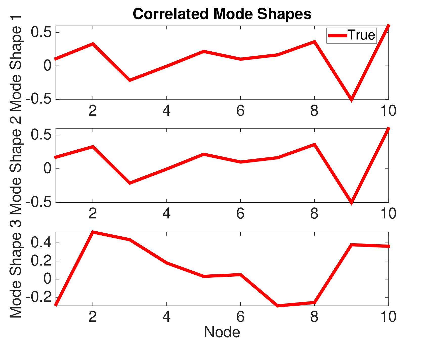 Figure 1
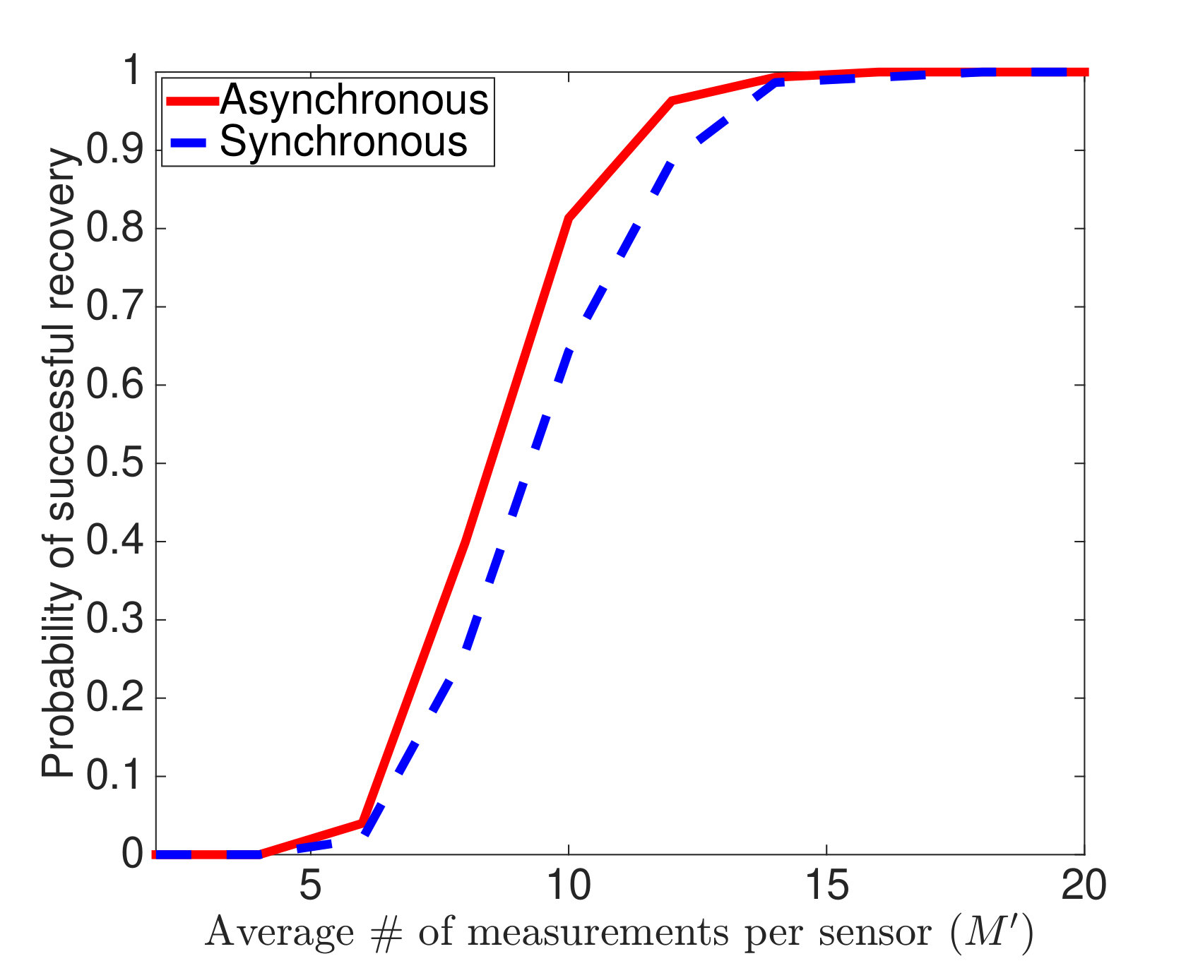 Figure 2
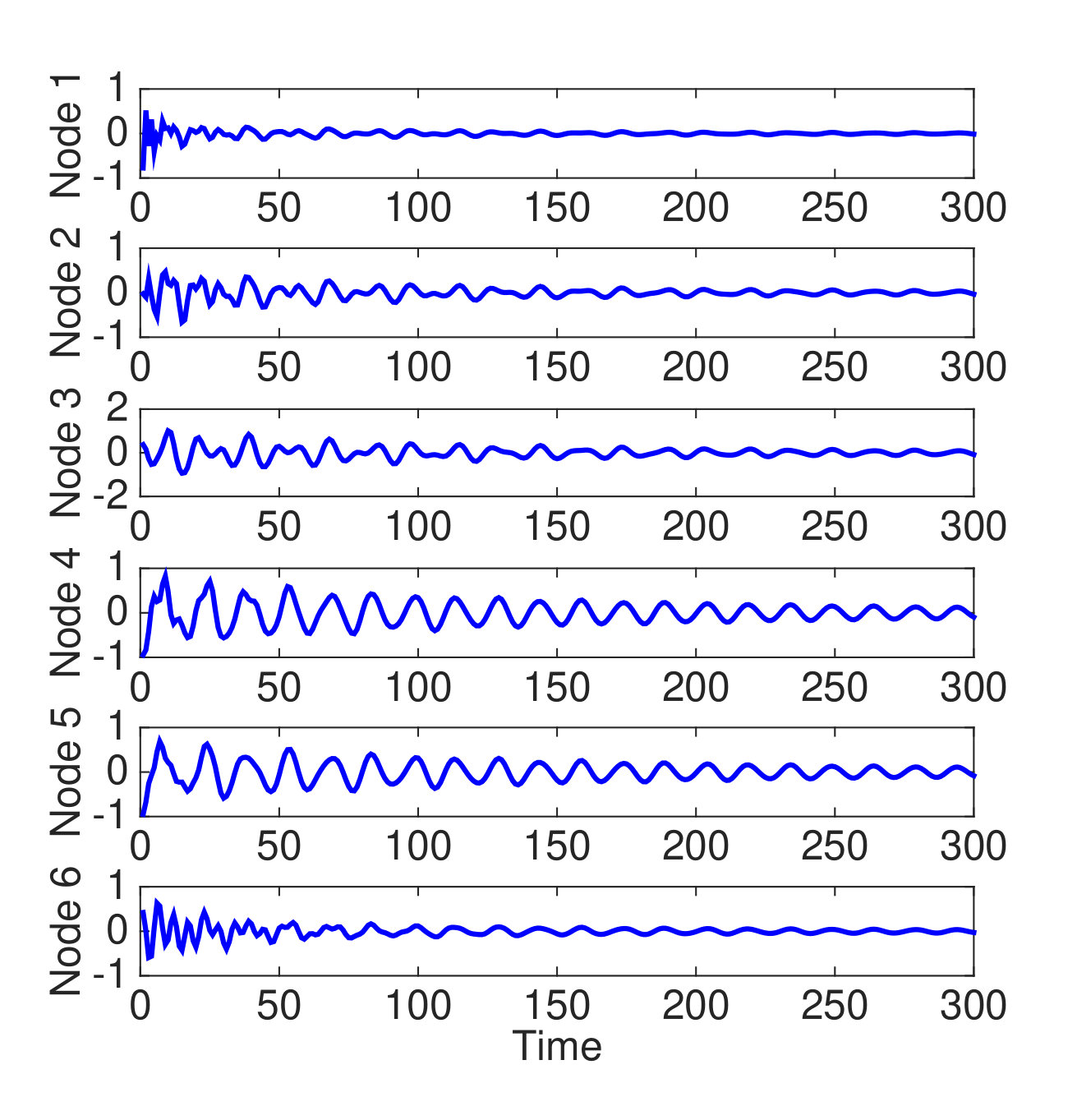 Figure 3
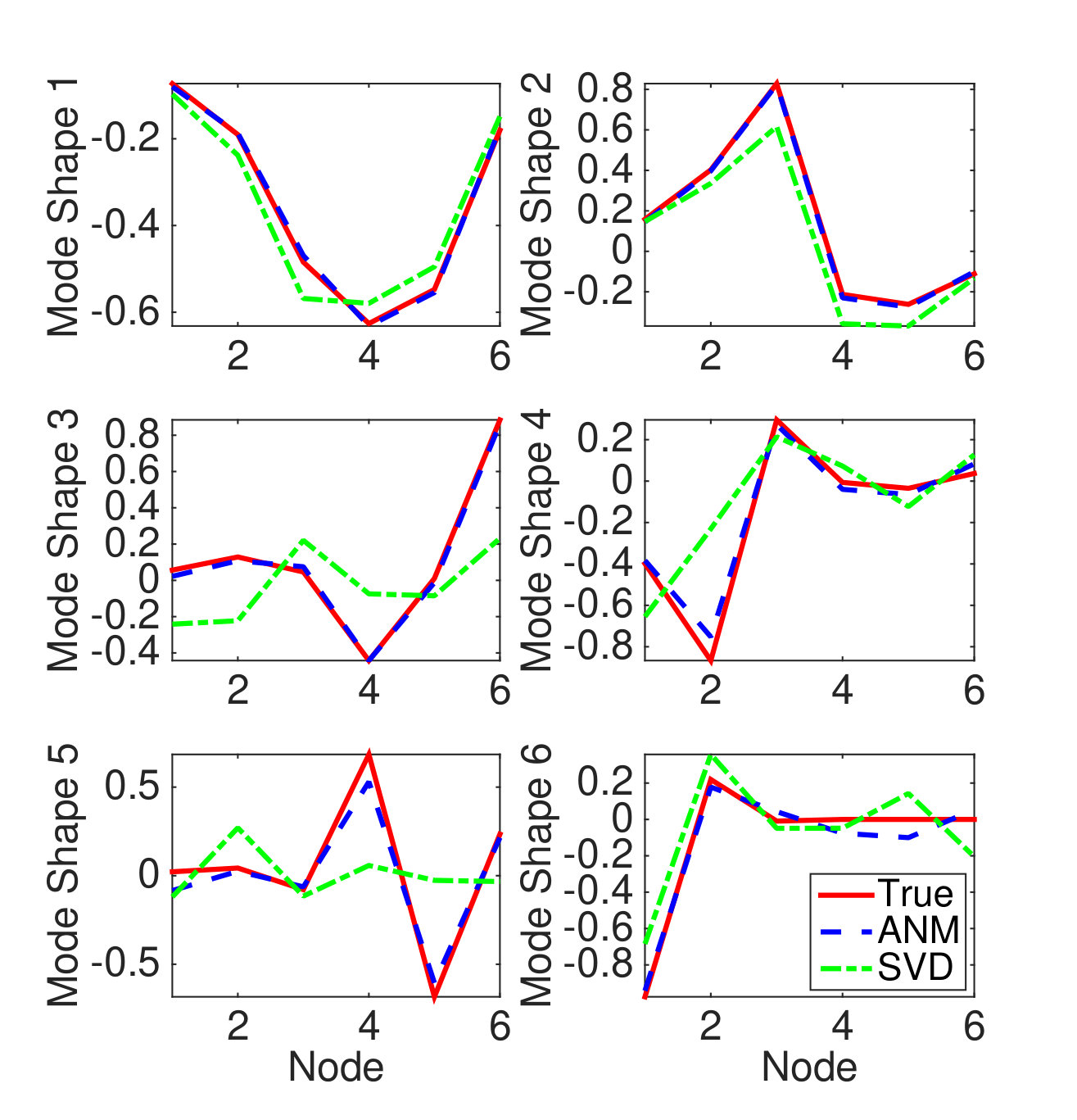 Figure 4
 Figure 5
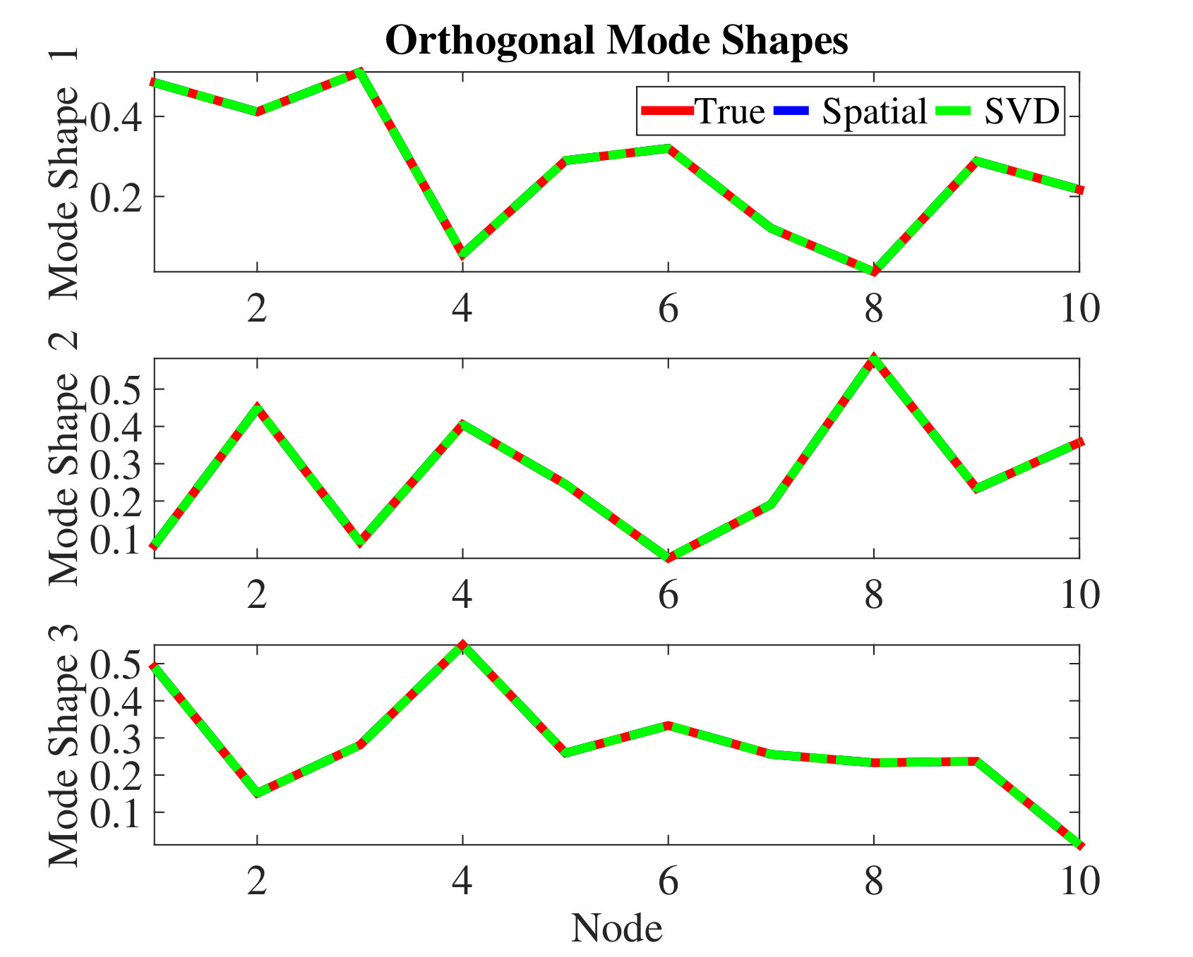 Figure 6
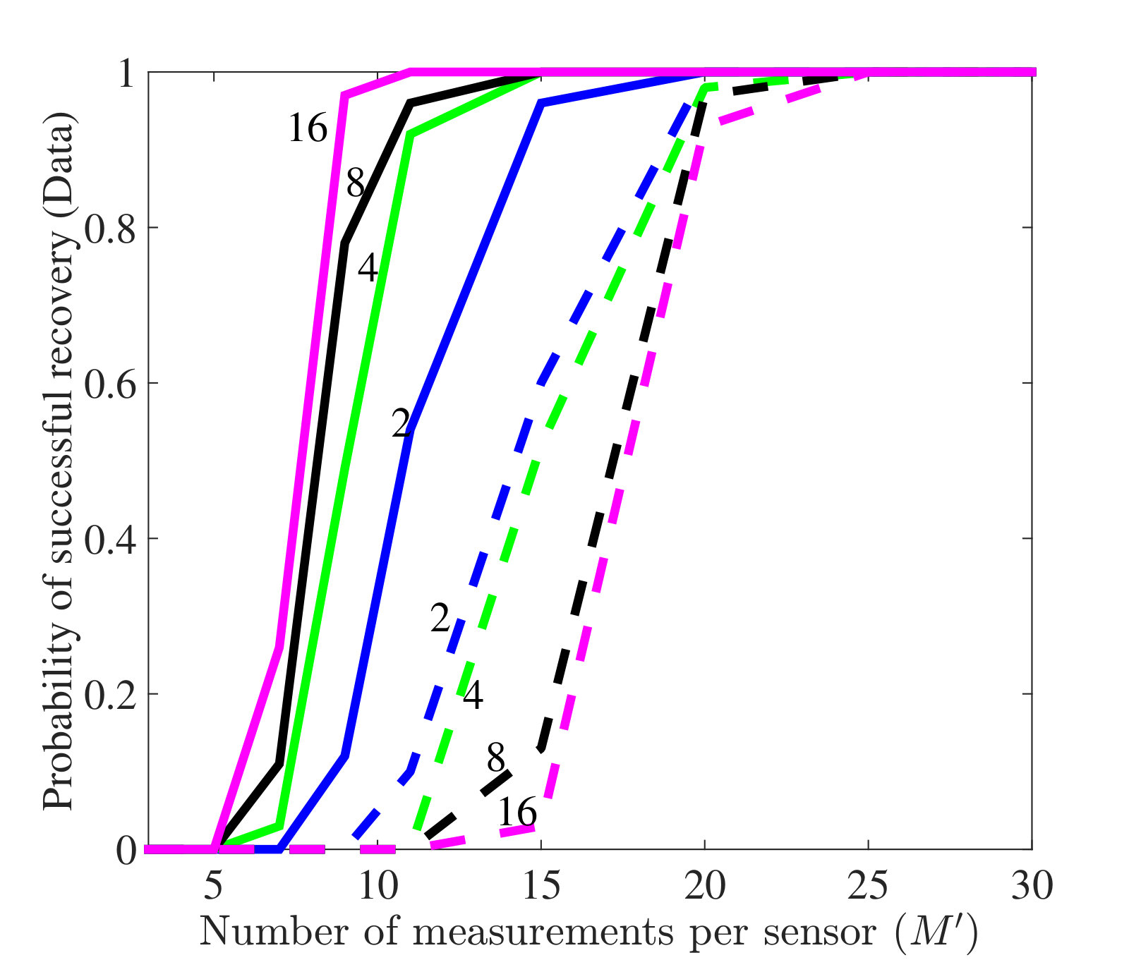 Figure 7
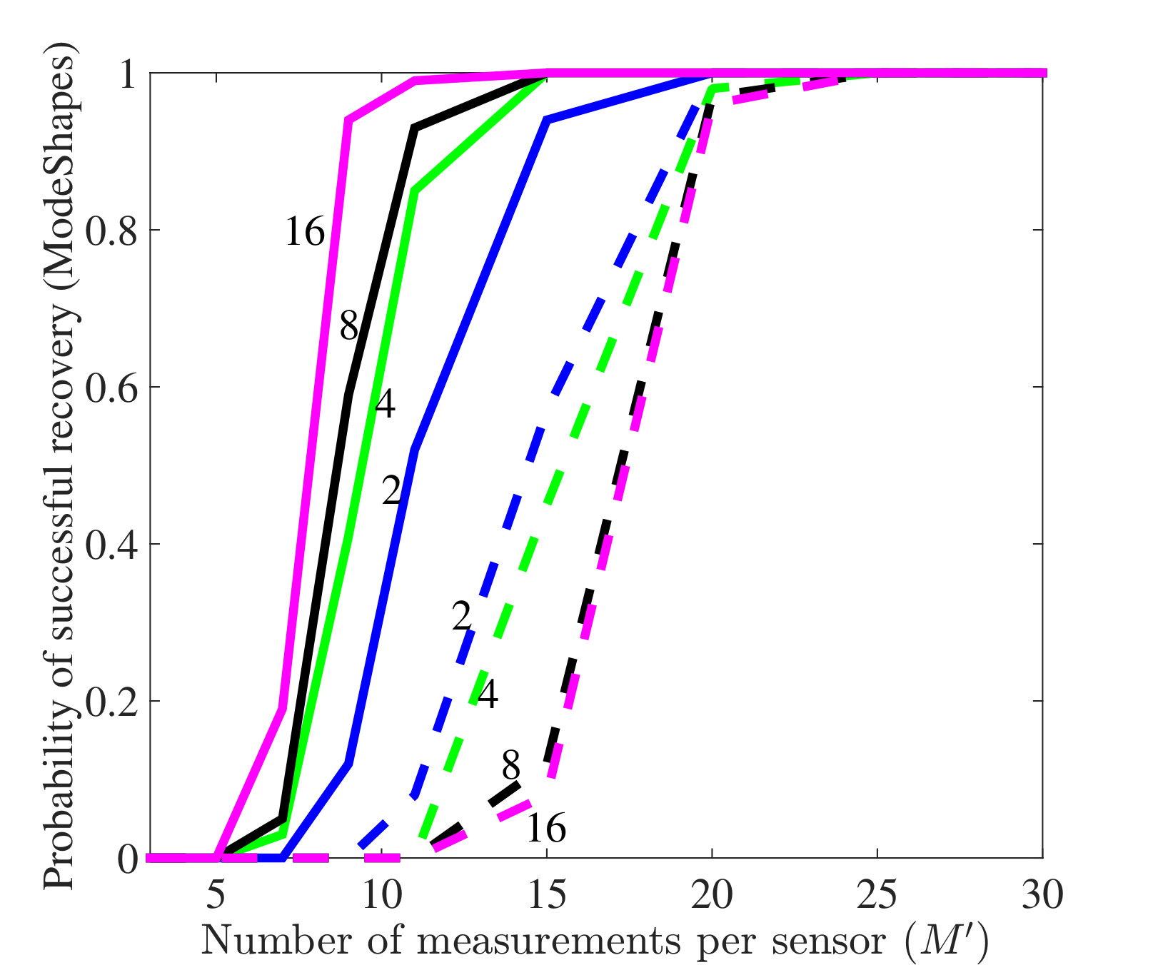 Figure 8
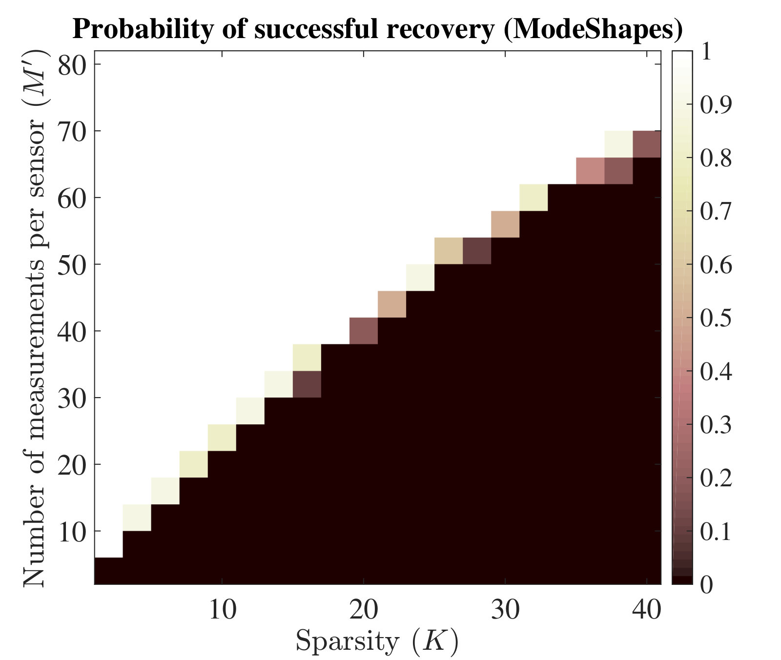 Figure 9
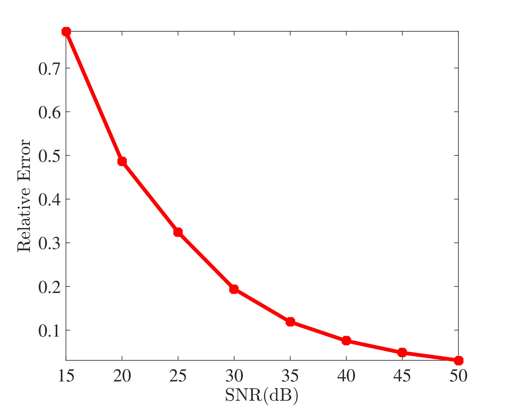 Figure 10
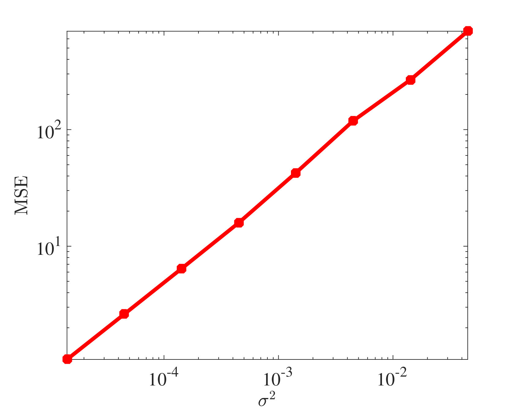 Figure 11
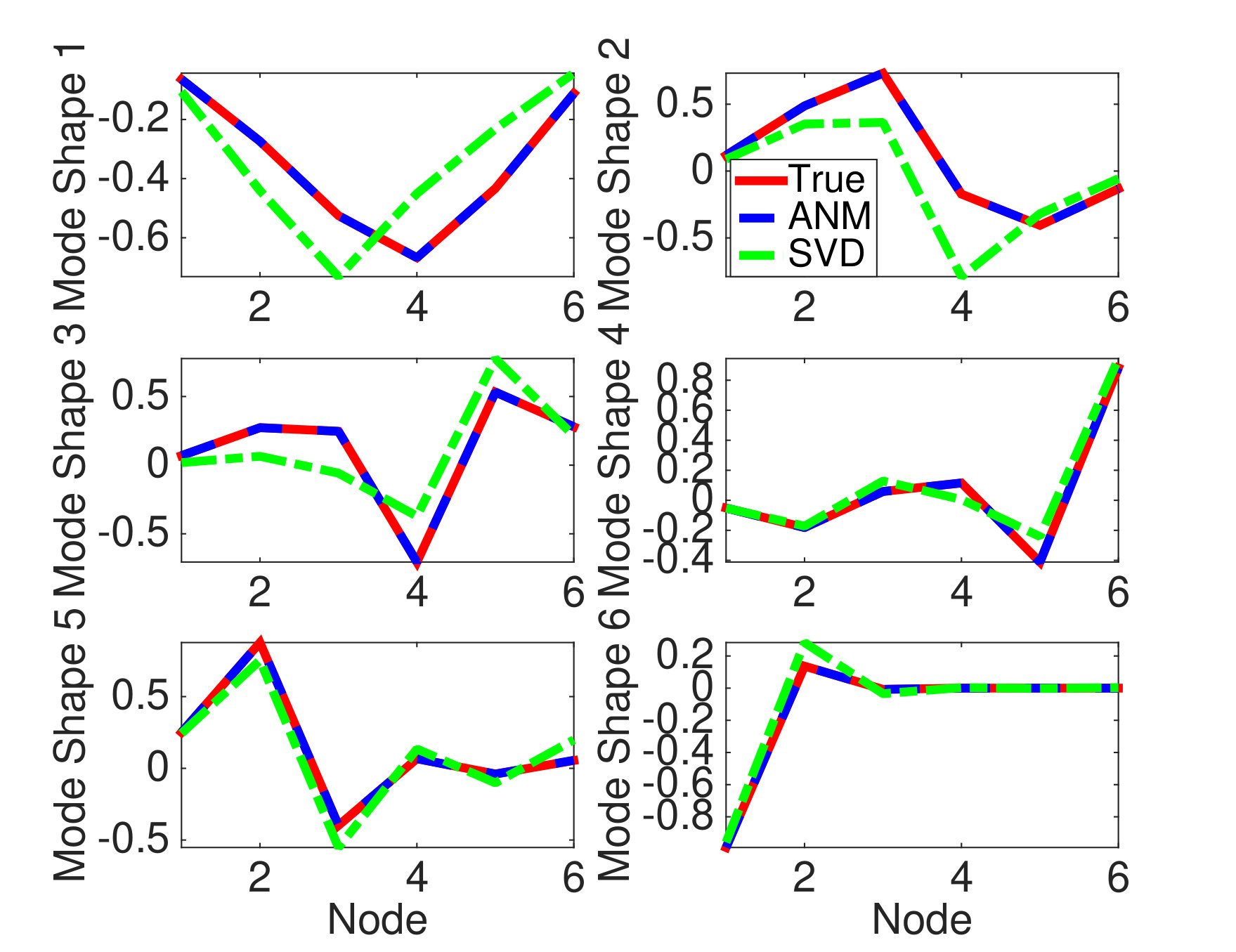 Figure 12
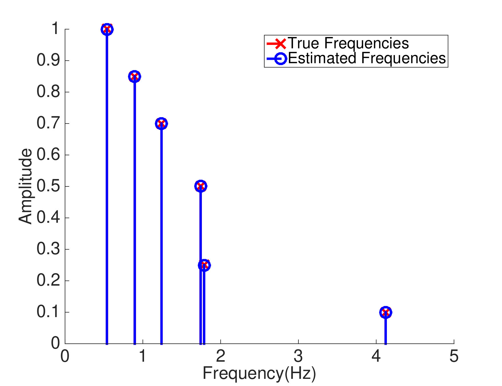 Figure 13
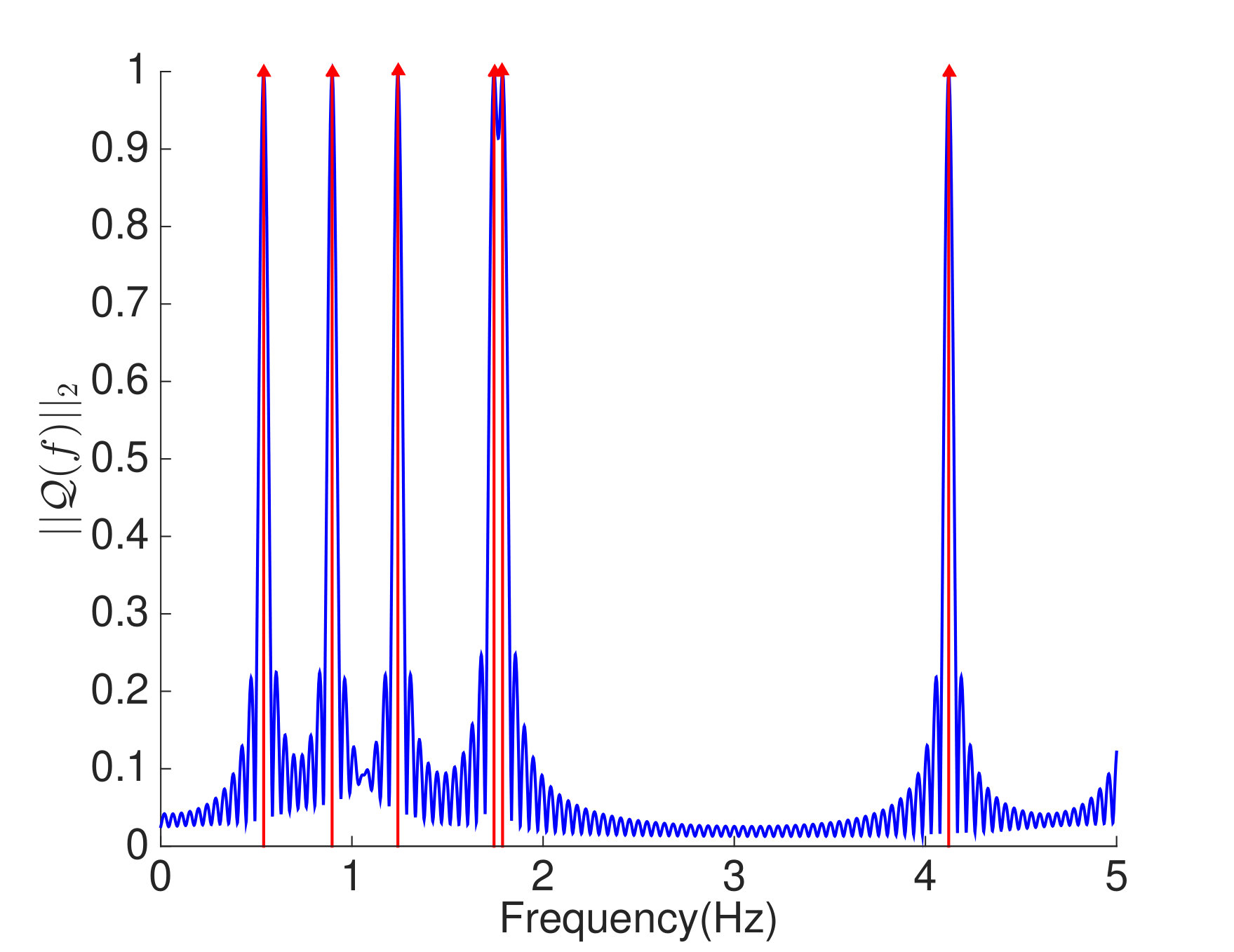 Figure 14
Peer Reviews
No public reviews on file for this paper yet. If you reviewed it on a platform where reviews are public (OpenReview, ICLR, NeurIPS, ICML), you can paste yours below so the community can read it here.
Videos
No videos yet. Explain this paper in a talk, walkthrough, or lecture? Add one.
Atomic Norm Minimization for Modal Analysis
from Random and Compressed Samples
Shuang Li, Dehui Yang, Gongguo Tang, and Michael B. Wakin Department of Electrical Engineering, Colorado School of Mines. Email: {shuangli,dyang,gtang,mwakin}@mines.edu
Abstract
Modal analysis is the process of estimating a system’s modal parameters such as its natural frequencies and mode shapes. One application of modal analysis is in structural health monitoring (SHM), where a network of sensors may be used to collect vibration data from a physical structure such as a building or bridge. There is a growing interest in developing automated techniques for SHM based on data collected in a wireless sensor network. In order to conserve power and extend battery life, however, it is desirable to minimize the amount of data that must be collected and transmitted in such a sensor network. In this paper, we highlight the fact that modal analysis can be formulated as an atomic norm minimization (ANM) problem, which can be solved efficiently and in some cases recover perfectly a structure’s mode shapes and frequencies. We survey a broad class of sampling and compression strategies that one might consider in a physical sensor network, and we provide bounds on the sample complexity of these compressive schemes in order to recover a structure’s mode shapes and frequencies via ANM. A main contribution of our paper is to establish a bound on the sample complexity of modal analysis with random temporal compression, and in this scenario we prove that the required number of samples per sensor can actually decrease as the number of sensors increases. We also extend an atomic norm denoising problem to the multiple measurement vector (MMV) setting in the case of uniform sampling.
1 Introduction
Modal analysis is the process of estimating a system’s modal parameters such as its natural frequencies, mode shapes, and damping factors. One application of modal analysis is in structural health monitoring (SHM), where a network of sensors may be used to collect vibration data from a physical structure such as a building or bridge. The vibration characteristics of a structure are captured in its modal parameters, which can be estimated from the recorded displacement data. Changes in these parameters over time may be indicative of damage to the structure. Modal analysis has been widely used in civil structures [1], space structures [2], acoustical instruments [3], and so on.
Due to the considerable time and expense required to perform manual inspections of physical structures, and the difficulty of repeating these inspections frequently, there is a growing interest in developing automated techniques for SHM based on data collected in a wireless sensor network. For example, one could envision a collection of battery-operated wireless sensors deployed across a structure that record vibrational displacements over time and then transmit this information to a central node for analysis. In order to conserve power and extend battery life, however, it is desirable to minimize the amount of data that must be collected and transmitted in such a sensor network [4].
In this paper, we highlight the fact that modal analysis can be formulated as an atomic norm minimization (ANM) problem, which can be solved efficiently and in some cases recover perfectly a structure’s mode shapes and frequencies. We survey several possible protocols for data collection, compression, and transmission, and we review the sampling requirements in each case. ANM generalizes the widely used -minimization framework for finding sparse solutions to underdetermined linear inverse problems [5]. It has recently been shown to be an efficient and powerful way for exactly recovering unobserved time-domain samples and identifying unknown frequencies in signals having sparse frequency spectra [6, 7, 8], in particular when the unknown frequencies are continuous-valued and do not belong to a discrete grid. Sampling guarantees have been established both in the single measurement vector (SMV) scenario [6, 9] and in the multiple measurement vector (MMV) scenario under a joint sparse model [10, 7]; these results characterize the number of uniform or random time-domain samples to achieve exact frequency localization as a function of the minimum separation between the unknown frequencies. In this sense, by achieving exact recovery, ANM can completely avoid the effects of basis mismatch [11, 12, 13] which can plague conventional grid-based compressive sensing techniques.
To provide context in this paper, we survey a broad class of sampling and compression strategies that one might consider in a physical sensor network, and we provide bounds on the sample complexity of these compressive schemes in order to recover a structure’s mode shapes and frequencies via ANM. In total, we consider five measurement schemes:
- •
uniform sampling, where vibration signals at each sensor are sampled synchronously at or above the Nyquist rate and transmitted without compression to a central node,
- •
synchronous random sampling, where vibration signals at each sensor are sampled randomly in time (as a subset of the Nyquist grid), but at the same time instants at each sensor,
- •
asynchronous random sampling, where vibration signals at each sensor are sampled randomly in time (as a subset of the Nyquist grid), at different time instants at each sensor,
- •
random temporal compression, where Nyquist-rate samples are compressed at each sensor via random matrix multiplication, before transmission to a central node, and
- •
random spatial compression, where Nyquist-rate samples are compressed en route to the central node.
Note that all sensors share the same Nyquist grid in each of these measurement schemes.
Modal analysis is a particular instance of the joint sparse frequency estimation problem, which has also been commonly studied in the context of direction-of-arrival (DOA) estimation [14]. Some conventional methods for joint sparse frequency estimation, such as MUSIC [15], can identify frequencies using a sample covariance matrix as long as a sufficient number of snapshots is given. However, as noted in [10], these methods usually assume that the source signals are spatially uncorrelated and their performance would decrease with source correlations. ANM does not have this limitation. Moreover, joint sparse frequency estimation techniques such as MUSIC do not naturally accommodate the sort of randomized sampling and compression protocols that we consider in this paper.
In this work, we explain how the results from [7, 10] can be interpreted in the context of exactly recovering a structure’s mode shapes and frequencies from uniform samples, synchronous random samples, and asynchronous random samples. These random sampling results have an unfortunate scaling, however, in that the number of samples per sensor actually increases as the number of sensors increases; intuition and simulations suggest that the opposite should be true. A main contribution of our paper, then, is to establish a bound on the sample complexity of modal analysis with random temporal compression, and in this scenario we prove that the required number of samples per sensor can actually decrease as the number of sensors increases. A similar phenomenon—that the estimation accuracy increases as the number of snapshots increases—occurs in covariance fitting methods for DOA estimation [14]. We also explain how our previous work [16] on super-resolution of complex exponentials from modulations with unknown waveforms can be used to establish a bound on the sample complexity of modal analysis with random spatial compression. For the noisy case, we extend the SMV atomic norm denoising problem in [17, 18] to an MMV atomic norm denoising problem in the case of uniform sampling. We derive theoretical guarantees for this MMV atomic norm denoising problem. Although we focus on modal analysis to put our analysis and simulations in a specific context, our results can apply to joint sparse frequency estimation more generally.
The remainder of this paper is organized as follows. In Section 2, we provide some background on modal analysis and on the atomic norm. In Section 3, we formulate our problem, and we characterize the ability of ANM to exactly recover a structure’s mode shapes and frequencies under each of the above five measurement schemes. We also provide a bound on the performance of ANM in the case of noisy, uniform samples. In Section 4, we present simulation results to illustrate some of the essential trends in the theoretical results and to demonstrate the favorable performance of ANM. We prove our main theorems in Section 5, and we make some concluding remarks in Section 6. The Appendix provides supplementary theoretical results.
2 Background
2.1 Modal analysis
For an degree-of-freedom linear time-invariant system [19], the second-order equations of motion which represent the dynamic behavior of the system can be formulated as
[TABLE]
where , and denote the mass, damping, and stiffness matrices, respectively. In this equation, represents a length- vector of displacement values at time , and represents the excitation force at the nodes. We will assume that each of the displacement values is associated with a wireless sensor node that can sample, record, and transmit that displacement value; as an example, one could equip each of the six boxcars shown in Fig. 1 with a displacement sensor.
As a simplification and as in [20], we consider systems in free vibration, where the forcing input and the system vibrates freely in response to some set of initial conditions.111One can also consider modal analysis with forced vibration [21, 22, 23, 24], when external forces such as an earthquake, wind, or vehicle loadings are applied. In this case, the general solution to (2.1) takes the form [25]
[TABLE]
where are a collection of mode shape vectors whose span characterizes the set of possible displacement profiles of the structure, and are modal responses in the form of monotone exponentially-decaying sinusoids:
[TABLE]
Here, and are determined by the initial conditions, and the number of nonzero amplitudes corresponds to the number of active modes. The parameters , , and denote the th damping ratio, the natural frequency, and the damped frequency, respectively, and these parameters along with the mode shapes are intrinsic properties of the system determined by the mass, damping, and stiffness matrices. Modal analysis refers to the identification of these parameters—particularly the mode shapes, damping ratios, and frequencies—from observations of the displacement vector .
In recent years, blind source separation (BSS) based methods have become very popular in modal analysis. The authors in [26] and [27] propose a new modal identification algorithm based on sparse component analysis (SCA) to deal with even the underdetermined case where sensors may be highly limited compared to the number of active modes. In [28], a novel decentralized modal identification method termed PARAllel FACtor (PARAFAC) based sparse BSS (PSBSS) method is proposed. Independent component analysis (ICA) is a powerful method to solve the BSS problem. Yang et al. present an ICA based method to identify the modal parameters of lightly and highly damped systems, even in cases with heavy noise and nonstationarity [29]. Despite the favorable empirical performance of these methods, few of them have been supported by theoretical analysis. In this paper, inspired by promising recent work in line spectrum estimation, we provide theoretical support for ANM as a powerful technique for modal analysis.
Meanwhile, over the past decade, the development of compressive sensing (CS) has highlighted the possibility of capturing essential signal information with sampling rates much lower than the Nyquist rate [30, 31, 32]. Exploring the possibility of using CS in modal analysis, Park et al. provide a theoretical analysis of a singular value decomposition (SVD) based technique for estimating a structure’s mode shapes in free vibration without damping [20]. The work in [20] builds upon a previous observation [33] that with a sufficiently large number of samples, the SVD technique can identify the mode shapes of systems with uniformly distributed mass (which leads to mutually orthogonal mode shapes) and light or no damping; as such, the results in [20] are limited to the assumption that the mode shapes are mutually orthogonal, which is not satisfied for general systems. In a more recent work, Yang et al. propose a BSS based method that can identify non-orthogonal mode shapes from video measurements [34]. The same group also develops another BSS based method to identify modal parameters from uniformly sub-Nyquist (temporally-aliased) video measurements [35]. Another recent work [36] also presents a new method based on a combination of CS and complexity pursuit (CP) to solve the modal identification problem.
In a very recent paper [9], Heckel and Soltanolkotabi consider solving a generalized line spectrum estimation problem with convex optimization. In particular, they recover a data vector from its compressed measurements using an ANM formulation that has been mentioned in [5]. Several different classes of random sensing matrices are considered for obtaining the measurements. The result for Gaussian random matrices in [9] can be viewed as a special case of our modal analysis result for random temporal compression (Theorem 3.4), where we have multiple measurement vectors and use a different sensing matrix for each measurement vector. Our analysis is inspired by their proof.
Finally, Lu et al. [37] propose a concatenated ANM approach for joint recovery of frequency sparse signals under a certain joint sparsity model. This problem differs from ours in the signal model, and the paper [37] does not establish theoretical bounds on the sample complexity.
2.2 The atomic norm
Frequency estimation from a mixture of complex sinusoids is a classical problem in signal processing. As mentioned in the introduction, ANM has recently been considered as a technique for solving this problem, both in the SMV () and MMV () scenarios. Under the right conditions, ANM can achieve exact frequency localization, avoiding the effects of basis mismatch which can plague grid-based techniques. In Section 3, we survey various formulations of the ANM problem that can be used with the various compressive measurement protocols for modal analysis. All of these formulations rely on the same core definition of an atomic norm, which is established in [7, 10] and repeated here.
Suppose each column of an data matrix is a spectrally sparse signal with distinct frequency components and denoted as
[TABLE]
Here, the vector
[TABLE]
corresponds to a collection of samples of a complex exponential signal with frequency . Note that we use “” and “” to denote transpose and conjugate transpose, respectively.
As shown in [7] and [10], one can define an atomic set to represent such a data matrix with each atom defined as
[TABLE]
where , with . The corresponding atomic set can be defined as
[TABLE]
The atomic norm of is then defined as
[TABLE]
where is the convex hull of . This atomic norm is equivalent to the solution of the following semidefinite program (SDP):
[TABLE]
where is the Hermitian Toeplitz matrix with the vector as its first column. denotes the trace of a square matrix. The proof of this SDP form can be found in [6, 7].
The dual norm of is defined as
[TABLE]
where is known as the dual polynomial. Above, corresponds to the real inner product between two matrices.
3 Main Result
3.1 Preliminaries
As in [20], we assume the structure has no damping () and that the real-valued displacement222Although we refer to displacement data in this work, the ANM method can also be applied to acceleration data. In particular, the ground truth acceleration signal vector will have the same form as (3.1) but with a different set of amplitudes . signal has been converted to its complex analytic form, which can be accomplished by using the Hilbert transform in practice [38, 39]. In this case, the ground truth displacement signal vector can be written as
[TABLE]
which is a superposition of complex sinusoids. Here, , , and are the complex amplitudes, frequencies, and mode shapes, respectively. We assume without loss of generality that the mode shapes are normalized333Equation (3.1) will hold with any choice of normalization for the mode shapes, as any rescaling of can be simply absorbed into . Any such renormalization can be applied after the Euclidean-normalized mode shapes are recovered and thus does not affect our results. A certain “mass normalization” is desired in some applications. Employing mass normalization requires either knowledge of the mass matrix or extra experiments [40]. such that . As in Section 2.1, denotes the number of sensors. Thus, is the displacement signal at the th sensor.
Because we assume that is an analytic signal, all .444It would not be difficult to extend our analysis to the case where the frequencies in (3.1) can be negative or positive: one would set and , which yields discrete frequencies , which is equivalent to the interval . Define . If one were to take regularly spaced Nyquist samples of at times
[TABLE]
where , and then stack the signal from the th sensor as the th column of a data matrix , one would have
[TABLE]
where with being the phase of the complex amplitude , are the discrete frequencies, are sampled complex exponentials as defined in (2.2), and are the atoms defined in (2.3). The ability to express as a linear combination of atoms from the atomic set inspires the use of ANM to recover from partial information, as we discuss below.
3.2 Modal analysis for noiseless signals
In this section, we survey a broad class of sampling and compression strategies that one might consider in a physical sensor network, and we provide bounds on the sample complexity of these compressive schemes in order to recover a structure’s mode shapes and frequencies via ANM.
The performance of ANM in these various scenarios will depend on the minimum separation of the discrete frequencies ’s, which is defined to be
[TABLE]
where is understood as the wrap-around distance on the unit circle.
We also note that, because each complex mode shape vector is multiplied by a complex amplitude in our model (3.1), recovery of these mode shapes and amplitudes is possible only up to a phase ambiguity. We denote our estimated mode shapes as and measure recovery performance using the absolute inner product . Because and are both normalized, achieving corresponds to exact recovery of the mode shape up to the unknown phase term.
3.2.1 Uniform sampling
As a baseline, we begin by considering a conventional data collection scheme, in which samples from each sensor are collected uniformly in time with sampling rate . In this case, the data matrix , defined in (3.3), is fully observed. In this section, we assume the samples are collected without noise; Section 3.3 revisits the uniform sampling scheme in the case of noisy samples.
To identify the mode shapes and frequencies in this scenario, it can be useful to consider the following ANM formulation:
[TABLE]
Although this problem has a trivial solution (namely , which is already available), solving this problem in a certain way can reveal information about the mode shapes and frequencies. In particular, (3.4) is equivalent to the following SDP
[TABLE]
Certain approaches to solving this SDP555In practice, one can use the CVX software package [41]. will return the dual solution directly. From this, following Proposition 1 in [7], one can formulate the dual polynomial to identify the frequencies and mode shapes. In particular, one can identify the frequencies by localizing where the dual polynomial achieves . Note that the data matrix can also be rewritten as
[TABLE]
Then, using the estimated data matrix and estimated frequencies , one can solve a least-squares problem to estimate the complex amplitudes and mode shapes:
[TABLE]
where denotes the pseudoinverse of the matrix . Because the true mode shapes are assumed to be normalized, we normalize the estimated mode shapes by setting and .
The following theorem is adapted from Theorem 4 in [10].
Theorem 3.1**.**
[10]** Assume the data matrix shown in (3.3) is obtained by uniformly sampling the displacement signal vector in time with a sampling interval . If the number of samples from each sensor satisfies
[TABLE]
then ANM perfectly recovers all frequencies and all mode shapes up to a phase ambiguity, i.e., .
This theorem indicates that more measurements are needed at each sensor for perfect recovery as the minimum separation decreases, i.e., as the true frequencies become closer to each other.666The resolution limit is commonly encountered in atomic norm minimization. A recent work [42] proposes a reweighted atomic norm minimization algorithm that can improve upon this resolution limit. As noted in Section 2.1, Park et al. [20] have provided a theoretical analysis of an SVD based technique for modal analysis. That work also considers uniform sampling and provides a bound on that is similar to what is required in (3.5). However, the analysis in [20] is limited to the case where the true mode shapes are mutually orthogonal, a condition that we do not require here. Moreover, the SVD guarantees apply only to approximate recovery of the mode shapes; as confirmed in Theorem 3.1, ANM can offer exact recovery of both the mode shapes and frequencies.
3.2.2 Synchronous random sampling
As a first alternative to conventional uniform sampling, we now consider the case where vibration signals at each sensor are sampled randomly in time, but at the same time instants at each sensor. We refer to this data collection scheme as synchronous random sampling.
To be specific, we suppose that the random sample times are chosen as a subset of the Nyquist grid; thus, the random samples are merely a subset of a collection of uniform samples. Equivalently, we suppose that we observe (which is defined in (3.3)) on a set of indices with and , where is defined in (3.2). Thus, each column of is observed at the same times, indexed by .
Denoting the observed matrix as , the ANM problem can be formulated as
[TABLE]
which is equivalent to the following SDP
[TABLE]
As in Section 3.2.1, one can solve the above SDP, obtain the estimated frequencies from the dual polynomial, and recover the mode shapes and amplitudes by solving a least-squares problem.
The following theorem from [10] shows that we can recover and estimate the frequencies accurately with high probability.
Theorem 3.2**.**
[10]** Suppose the data matrix is observed on the index set , with selected uniformly at random as a subset of . Assume that are independent random vectors with , chosen independently of the fixed amplitudes . That is, each is sampled independently from a zero-mean distribution on the complex hyper-sphere; this distribution may vary with . If , then there exists a numerical constant such that
[TABLE]
is sufficient to guarantee that we can exactly recover via (3.6) and perfectly recover the frequencies and mode shapes up to a phase ambiguity with probability at least .
The above theorem indicates that the number of measurements needed from each sensor for perfect recovery scales almost linearly with the number of active modes . The number of random samples per sensor also increases logarithmically with , the number of underlying uniform samples in . The lower limit on is similar to what appears in Theorem 3.1 for the uniform sampling case. Thus, the total duration over which the signals must be observed does not change. However, what is significant is that in many cases the lower bound on will be smaller than , which confirms that in general during this time span it is not necessary to fully sample the uniform data matrix ; sensing and communication costs can be reduced by randomly subsampling this matrix.
Because its derivation relies on concentration arguments such as Hoeffding’s inequality, Theorem 3.2 does assume the mode shapes to be generated randomly, which is not physically plausible. Moreover, this result actually requires the number of measurements per sensor to increase (albeit logarithmically) as the number of sensors increases. However, intuition suggests that the opposite should be true: the signals share a common structure (analogous to a joint sparse model [43] in distributed compressive sensing), and observing more signals gives more information about this common structure.
It is reasonable to expect that one will actually need fewer measurements per sensor as the number of sensors increases. This is supported by simulations (not shown in this paper), and it remains an open question to support this with theory for the case of synchronous random sampling.777After the initial submission of this manuscript, [44] has appeared as a complement to [10] and improves upon the sample complexity in Theorem 3.2 under a different random assumption on the mode shapes.
3.2.3 Asynchronous random sampling
We now consider the case where vibration signals at each sensor are sampled randomly in time, but at different time instants at each sensor. We refer to this data collection scheme as asynchronous random sampling. To be specific, suppose that we observe on the indices . This observation model allows each column of to be observed at different times, all of which are still restricted to be drawn from the uniform sampling grid , defined in (3.2).
Recovery of the full data matrix from asynchronous random samples is analogous to the conventional matrix completion problem. This problem can be solved using ANM with the same formulation as in (3.6) but with replaced by . The following theorem from [7] shows that one can again recover and estimate the frequencies and mode shapes accurately with high probability.888An explicit proof of Theorem 3.3, which concerns MMV ANM, is not included in [7]. We do note that essentially the same conclusion holds if one applies SMV ANM and uses a union bound over the sensors.
Theorem 3.3**.**
[7]** Suppose the data matrix is observed on the index set , which is selected uniformly at random. Assume the signs are drawn independently from the uniform distribution on the complex unit circle (and independently of the fixed amplitudes ) and that . Then there exists a numerical constant such that
[TABLE]
is sufficient to guarantee that we can exactly recover via (3.6) and exactly recover the frequencies and mode shapes up to a phase ambiguity with probability at least .
Up to small differences in the logarithmic factors, the total number of samples required in Theorem 3.3 is comparable to the number of sensors times the number of samples per sensor required in Theorem 3.2. Many of the same comments on the theorem apply here, including the use of a (different) randomness assumption on the mode shapes, and the fact that the required average number of measurements per sensor again increases logarithmically as the number of sensors increases. Again, the lower limit on is similar to what happens in Theorem 3.1, and so the total duration over which the signals must be observed does not change. However, during this time span the requisite number of asynchronous random samples may be far lower than the number of uniform samples demanded by the Nyquist rate.
Comparing the logarithmic terms in the right hand sides of (3.7) and (3.8), we do see that the measurement requirement is slightly stronger for asynchronous random sampling than for synchronous random sampling. However, simulations (e.g., Fig. 3(b)) indicate that the opposite may be true. It remains an open question to support this with theory.
3.2.4 Random temporal compression
Inspired by alternatives to random sampling that have been considered in CS, we now consider the case where the displacement signal at each sensor is compressed via random matrix multiplication before being transmitted to a central node. We refer to this as random temporal compression. This compression strategy was also considered in [20], which provided a theoretical analysis of an SVD based technique for modal analysis.
Let be the th column of the data matrix , and let be a compressive matrix generated randomly with independent and identically distributed (i.i.d.) Gaussian entries. At each sensor, assume that we compute the measurements
[TABLE]
At the central node, the problem of recovering the original data matrix from the compressed measurements can be formulated as
[TABLE]
which is equivalent to
[TABLE]
As in Section 3.2.1, one can solve the above SDP, obtain the estimated frequencies from the dual polynomial, and recover the mode shapes and amplitudes by solving a least-squares problem. We have the following result.
Theorem 3.4**.**
Suppose are independently drawn random matrices with i.i.d. Gaussian entries having mean zero and variance . Assume that the true frequencies satisfy the minimum separation condition
[TABLE]
Then there exists a numerical constant such that if
[TABLE]
* is the unique optimal solution of the ANM problem (3.9) and we can exactly recover the frequencies and mode shapes up to a phase ambiguity with probability at least .*
We prove Theorem 3.4 in Section 5.2, extending analysis from Theorem 2 in [9], which concerned the SMV () version of this problem.
From Theorem 3.4, we see that modal analysis is possible in the random temporal compression scenario using a number of measurements per sensor that scales linearly with the number of active modes . One logarithmic term remains in this bound (3.11), while some of the other logarithmic terms appearing in (3.7) and (3.8) have disappeared. Expressing the failure probability as for easier comparison with Theorems 3.2 and 3.3, we see that when
[TABLE]
exact recovery of the mode shapes and frequencies is possible with probability at least . In the first term inside this expression, the number of measurements per sensor actually decreases as the number of sensors increases, a contrast with Theorem 3.2 and 3.3 where the opposite trend holds. We note that the benefit of increasing the number of sensors comes from the fact that in the setup of Theorem 3.4, each sensor uses a different measurement matrix . When the second term in (3.12) dominates, the number of measurements per sensor still does not increase with . Similar to the random sampling schemes, the total duration over which the signals must be observed does not change, but within this time span significant compression may be possible.
Also in contrast with Theorems 3.2 and 3.3, Theorem 3.4 requires no randomness assumption on the mode shapes. This allows for its use in practical scenarios, where in general mode shapes will not be generated randomly. It would be interesting to remove the randomness condition from Theorems 3.2 and 3.3; we leave this as a question for future work.
3.2.5 Random spatial compression
As a final strategy to compress the data matrix, we consider the scenario where each sensor modulates its sample value by a random number at each time sample, then the sensors transmit these values coherently to the central node, where the modulated values add to result in a single measurement vector. As discussed in [45], such randomized spatial aggregation of the measurements can be achieved as part of using phase-coherent analog transmissions to the base station. This strategy is sometimes referred to as compressive wireless sensing; we refer to it as random spatial compression.
In random spatial compression, the collected measurements can be expressed as
[TABLE]
where and is the th canonical basis vector. This allows us to formulate the modal analysis problem as an ANM problem:
[TABLE]
which is equivalent to
[TABLE]
As in Section 3.2.1, one can solve the above SDP, obtain the estimated frequencies from the dual polynomial, and recover the mode shapes and amplitudes by solving a least-squares problem. The following theorem follows from our previous work [16] on super-resolution of complex exponentials from modulations with unknown waveforms.
Theorem 3.5**.**
[16]** Suppose we observe the data matrix with the above random spatial compression scheme. Assume that the random vectors are i.i.d. samples from an isotropic and incoherent distribution (see [16] for details). Also, suppose that are drawn i.i.d. from the uniform distribution on the complex unit sphere and that the minimum separation condition (3.10) is satisfied. Then there exists a numerical constant such that999Note that the bound in (3.14) contains on both sides. One could remove from the right hand side using the Lambert W-function as in [46, (64)–(66)]. Here, we prefer the form in (3.14) for simplicity and to highlight the relationship between and .
[TABLE]
is sufficient to guarantee that we can exactly recover via (3.13) and exactly recover the frequencies and mode shapes up to a phase ambiguity with probability at least .
In random spatial compression, the central node receives exactly one compressed measurement at each time instant. Thus, the number of time samples equals the total number of compressed measurements. Thus, Theorem 3.5 states that it is sufficient for the total number of compressed measurements to scale essentially linearly with (as long as (3.10) is also satisfied). Since is the number of active modes and is the number of sensors (and thus the length of each unknown mode shape), the number of unknown degrees of freedom in this problem scales with . In this sense, the result in Theorem 3.5 compares favorably with those in Theorems 3.2, 3.3, and 3.4. Theorem 3.5 does require a randomness assumption on the mode shapes.
We note that, in some applications, once (3.10) is satisfied (which imposes a lower bound on that is comparable to what appears in Theorems 3.1–3.4), it could be the case that (3.14) is also satisfied. In this case, the same uniform data matrix that suffices for perfect recovery according to Theorem 3.1 can be completely compressed in the spatial dimension, reducing the total number of samples from to . Thus, significant savings may be possible in structures where the number of sensors is large. Indeed, up to the point where (3.14) becomes a stronger condition than (3.10), one could continue adding sensors without increasing the requisite number of compressed samples.
3.3 Modal analysis for noisy signals
In this section, we revisit the uniform sampling scenario where a data matrix is fully observed, but we now consider the case where the samples are corrupted by additive white Gaussian noise. While the analysis in this section may be of its own independent interest, it is also used in our proof of Theorem 3.4.
We consider observations of the form , where the entries of satisfy , and we consider the following atomic norm denoising problem:
[TABLE]
The theorem below provides an upper bound on the recovery error in Frobenius norm and is proved in Section 5.3.
Theorem 3.6**.**
Suppose the true data matrix is given as in (3.3) with the true frequencies satisfying the minimum separation condition (3.10). Given the noisy data , where the entries of are i.i.d. complex Gaussian random variables which satisfy , the estimate obtained by solving the atomic norm denoising problem (3.15) (with regularizing parameter and with chosen sufficiently large) will satisfy
[TABLE]
with probability at least for a numerical constant .
Corollary 3.1**.**
Under the assumptions of Theorem 3.6, the estimate obtained by solving the atomic norm denoising problem (3.15) (with regularizing parameter and with chosen sufficiently large) will satisfy
[TABLE]
Note that Theorem 3.6 provides a bound which extends the SMV case in [18] to the MMV case. Corollary 3.1 is a direct consequence of Theorem 3.6 and is proved in Section 5.4. The above MMV atomic norm denoising problem (3.15) is also considered in [7]. However, there the authors provide only an asymptotic bound on .
4 Simulation Results
In this section, we present some experiments on synthetic data to exhibit the performance of ANM based modal analysis in the various sampling and compression scenarios.101010We use ADMM [7] to solve the atomic norm denoising problem in Section 4.5. All other simulations are implemented with CVX [41]. We use the modal assurance criterion (MAC) to evaluate the quality of recovered mode shapes, which is defined as
[TABLE]
where is the th estimated mode shape and is the th true mode shape.111111To correctly pair the recovered mode shapes with the true ones, we assume the true frequencies are in ascending order, and we adopt the same convention for the estimated frequencies. A value of would indicate perfect recovery of the true mode shape. We consider mode shape recovery to be a success if for all . We consider data matrix recovery to be a success if .
4.1 Uniform sampling
As mentioned in Section 3.2.1, the full data, uniform sampling case has previously been considered in [10]. In this experiment, we compare the ANM based algorithm with the SVD based algorithm from [20] on a simple 6-degree-of-freedom boxcar system. The boxcar system is shown in Fig. 1. We consider this undamped system under the context of free vibration. The system parameters are set as follows: the masses are kg, and the stiffness values are , , , N/m. Thus, the mass, damping and stiffness matrices in (2.1) are given as , , and
[TABLE]
respectively. The true mode shapes and natural frequencies of this system can be obtained from the (normalized) generalized eigenvectors and square root of the generalized eigenvalues of the stiffness matrix and mass matrix . In particular, the true frequencies are , , , , , and Hz. We collect uniform samples from this system with sampling interval , where . The amplitudes are set as , , , , and . We apply both ANM and SVD to the obtained data matrix to identify the modal parameters of this boxcar system. (Note that the SVD based algorithm only estimates the mode shapes and not the frequencies.) Figure 2(a) shows how the dual polynomial from ANM can be used to localize the frequencies. In particular, we identify the frequencies by identifying where the dual polynomial achieves . The true frequencies and estimated frequencies are presented in Fig. 2(b). The estimated mode shapes from the two algorithms are illustrated in Fig. 2(c). As mentioned in Section 2.1, the SVD based algorithm can only return mode shape estimates that are mutually orthogonal (in fact they are orthogonal singular vectors of the data matrix). The true mode shapes in this experiment are not orthogonal, which hampers the performance of the SVD. The ANM algorithm is not restricted to returning orthogonal mode shape estimates, and in this experiment it recovers the mode shapes perfectly. In particular, the MAC for AMN is , while the MAC for SVD is .
In this experiment, the minimum separation . Theorem 3.1 guarantees that perfect recovery is possible via ANM when . We see perfect recovery in this simulation with uniform samples.
In the following sections, for convenience we will use random mode shapes and/or discrete frequencies to test the ANM based algorithms.
4.2 Asynchronous vs. synchronous random sampling
In this experiment, we compare the performance of asynchronous and synchronous random sampling in a case where the mode shapes are randomly generated but also correlated.121212We generate the first and third mode shapes randomly with i.i.d. Gaussian entries and then normalize. The second mode shape is generated by slightly perturbing the first mode shape and then normalizing. An example of such correlated mode shapes is shown in Fig. 3(a). (Only the first two mode shapes are correlated.) The true discrete frequencies are set to , , and . We collect uniform samples from each sensor. However, from these, on average, we keep only random samples from each sensor, where the value for ranges from to . In the case of synchronous random sampling, we keep exactly samples from each sensor at the same times. In the case of asynchronous random sampling, we generate uniformly at random, with .
Other parameters are set the same as in Section 4.1. We perform 300 trials (each with a new set of mode shapes) for each value of . Figure 3(b) shows that when compared with synchronous sampling, asynchronous random sampling needs fewer observed measurements to achieve the same probability of successful recovery. This observation is reasonable (given the additional diversity in the asynchronous observations) but stands in contrast with the relative difference between the theoretical bounds in Theorems 3.2 and 3.3. More work may be needed to theoretically characterize the performance difference between asynchronous and synchronous random sampling.
4.3 Random temporal compression
In the next set of experiments, we generate a series of random matrices to compress a set of uniform samples at each sensor. In the first experiment, we recover the data matrix and mode shapes both jointly (via the MMV approach from (3.9)) and separately (by solving separate SMV problems) to show the advantage of joint recovery. We choose between and and perform 100 trials for each value of . We use random mode shapes, all generated with i.i.d. Gaussian entries and then normalized. The true discrete frequencies are set to , , and , giving a separation of , which is slightly smaller than the separation condition prescribed in (3.10). Figures 4(a), (b) show the probability of successful recovery for the data matrix and mode shapes, respectively, when we use separate ANM (dashed lines) and joint ANM (solid lines). The number on each line denotes the number of sensors used in the experiments. It can be seen that joint recovery outperforms separate recovery significantly. Moreover, these results also indicate that the number of sensors has an important effect on the performance of joint recovery. In particular, for a given number of measurements , the probability of successful joint recovery will increase as the number of sensors increases, which is consistent with our theoretical analysis. In contrast, the probability of successful separate recovery will decrease.
In the second experiment, we set the number of sensors to be and investigate the minimal number of measurements per sensor needed for perfect joint recovery with various numbers of active modes . The true mode shapes are generated randomly and we set . For each value of , we randomly pick discrete frequencies from a frequency set , where . The amplitudes are chosen randomly from the uniform distribution between [math] and . It can be seen in Fig. 4(c) that the minimal number of measurements needed by each sensor for perfect recovery does scale roughly linearly with the number of active modes , as indicated in Theorem 3.4.
4.4 Random spatial compression
Using the same parameters as in Section 4.2, we simulate the random spatial compression strategy with ANM based modal analysis and compare to the SVD algorithm studied in [20], which we apply to a full data matrix. We generate mode shapes randomly, testing both orthogonal mode shapes and correlated mode shapes. It can be seen from Fig. 5(a), (b) that the SVD based method performs poorly when the mode shapes are correlated. However, the proposed ANM based algorithm performs well in both cases. Note that although SVD based method performs very well when the mode shapes are orthogonal, this is using samples while the ANM based algorithm uses only spatially compressed measurements to recover both the mode shapes and the frequencies.
4.5 Noisy data
Finally, we simulate the atomic norm denoising problem presented in Section 3.3. We assume the entries of are i.i.d. random variables from the distribution . We set the signal-to-noise ratio (SNR) between and dB, which corresponds to values of between and . We perform 50 trials for each value of , with random mode shapes in each trial. The regularization parameter is set to with and . Other parameters are set the same as in Section 4.2. We define and as the mean square error (MSE) and relative error, respectively. It can be seen in Fig. 6(a) that the MSE is linearly correlated with , which is consistent with the theory in Section 3.3. We also present Fig. 6(b) to illustrate how the relative error behaves with different noise levels.
5 Proofs
In this section, we will prove Theorem 3.4, Theorem 3.6, and Corollary 3.1. Some proof techniques are inspired by the work in [5, 9, 17, 18].
5.1 Convex analysis
We first review some basic concepts from convex analysis [47]. A set is a cone if
[TABLE]
where is a nonnegative constant. is a convex cone if
[TABLE]
holds for any and . The polar cone of a cone is
[TABLE]
The tangent cone and normal cone at with respect to the scaled unit ball are defined as
[TABLE]
and
[TABLE]
respectively. Note that the tangent cone is the set of descent directions of the atomic norm at . The normal cone is the polar cone of the tangent cone and vice-versa.
Let be a subset of , where denotes the unit sphere. Then, the Gaussian width of is
[TABLE]
where is a Gaussian matrix with i.i.d. entries from the distribution .
5.2 Proof of Theorem 3.4
We start by showing that the number of measurements needed for perfect recovery can be lower bounded with a Gaussian width in Section 5.2.1. Then, we upper bound the Gaussian width with the expectation of the recovery error obtained from the atomic norm denoising problem (3.15) in Section 5.2.2.
5.2.1 Bounding with a Gaussian width
It can be shown that the ANM problem in (3.9) is equivalent to the following optimization problem
[TABLE]
In particular, the above equivalent optimization problem can be obtained by eliminating the equality constraints in (3.9). Let with . It can be seen that the two optimization problems are equivalent.
Let . With a slight abuse of notation, we define
[TABLE]
as a set of matrices with columns belonging to the null space of the corresponding sensing matrix. We also define a block diagonal matrix corresponding to a matrix as
[TABLE]
Inspired by [5], we have the following proposition which gives us an optimal condition for exact recovery.
Proposition 1**.**
* is the unique optimal solution to the ANM (3.9) if and only if*
[TABLE]
Proof.
On one hand, if is the unique optimal solution, then holds for all . It follows that . Thus, we can get
On the other hand, if , then, for all , i.e., we have . Thus, is the unique optimal solution. ∎
Define , where . It can be seen that is a subset of the unit sphere. According to Proposition 1, to show that is the unique optimal solution to (3.9), we hope to demonstrate that holds for any , i.e.,
[TABLE]
which will hold if
[TABLE]
Therefore, we need to show
[TABLE]
where , and as is defined in (5.6). Note that we have since is in a subset of the unit sphere.
Next, we will show that holds for all with high probability. It then follows that is the unique optimal solution of ANM (3.9).
Theorem 5.1**.**
Let be a random matrix with i.i.d Gaussian entries which satisfy . Let be a subset of . For all , define as (5.6). Then, we have
[TABLE]
where and is the Gaussian width of defined in (5.1).
Remark 5.1**.**
The above theorem is based on Gordon’s work [48], and provides us a lower bound for the minimum gain of the operator restricted to a set . The proof of this theorem is given in Appendix A.1.
Corollary 5.1**.**
Let be a random matrix with i.i.d. Gaussian entries which satisfy . Define as a subset of the unit sphere. Then, is the unique optimal solution of ANM (3.9) with probability at least if
[TABLE]
Remark 5.2**.**
Corollary 5.1 is an immediate consequence of Theorem 5.1. It can be seen that the number of measurements needed for exact recovery can be lower bounded by a Gaussian width. The proof details (presented in Appendix A.2) are based on a Gaussian concentration inequality [49].
5.2.2 Bounding the Gaussian width
This section is dedicated to finding an upper bound on . First, we define the mean-square distance of a set as
[TABLE]
Inspired by the work in [5] and [9], we have
[TABLE]
where the first two inequalities follow from Proposition 3.6 in [5] and Jensen’s inequality, respectively. The third equality and last inequality can be found in equation (67) in [9] while the last equality comes from Theorem 1.1 in [50]. Note that is the polar cone of , as defined at the beginning of Section 5.1. Here, is the solution to the MMV atomic norm denoising problem (3.15) with being the regularization parameter. With the inequality given in (3.17), we have
[TABLE]
which implies
[TABLE]
Thus, plugging (5.8) into (5.7), we can get (3.11) and finish the proof of Theorem 3.4. ∎
5.3 Proof of Theorem 3.6
In this section, we prove Theorem 3.6 by extending the results in [17] and [18] to the MMV case. For the SMV case, it is shown in [17] that a good choice of the regularization parameter can achieve accelerated convergence rates. Inspired by their choice of the regularization parameter, we use
[TABLE]
in the MMV atomic norm denoising problem (3.15). Here, is some constant which ultimately must be set large enough to enable the proof of Lemma 5.6, and is a complex Gaussian matrix. To set , we need to find an upper bound for .
5.3.1 Bounding
Lemma 5.1**.**
Let be a random matrix with i.i.d. complex Gaussian entries from the distribution . Then, there exists a numerical constant such that
[TABLE]
Proof.
According to the definition of the dual atomic norm in (2.6), we have
[TABLE]
where the polynomial is defined as
[TABLE]
For all we have
[TABLE]
by using the mean value theorem and Bernstein’s inequality for polynomials [51]. By letting take any of the values , we have
[TABLE]
It follows that
[TABLE]
where the last inequality holds if . Then, we get
[TABLE]
and
[TABLE]
Define
[TABLE]
for . It can be seen that is complex Gaussian variable satisfying since the entries of satisfy . Then, we have
[TABLE]
where the last inequality uses the result that , see Lemma 5 in [17].
Choosing gives
[TABLE]
Note that is a constant which belongs to when is large. ∎
5.3.2 Bounding
Now, we can set the regularizing parameter in the MMV atomic norm denoising problem (3.15) as for some . Then
[TABLE]
holds with high probability. In particular, we have the following lemma.
Lemma 5.2**.**
[TABLE]
Proof.
As is shown in (5.9), letting , we have
[TABLE]
It can be seen that is stochastically upper bounded by a zero-mean Gaussian random variable with variance [9]. Then, for any , we have
[TABLE]
Let , we can get
[TABLE]
where the first inequality comes from the union bound. ∎
The following lemma derived from convex analysis provides optimality conditions for to be the solution of (3.15).
Lemma 5.3**.**
(Optimality Conditions): is the solution of (3.15) if and only if
, 2. 2.
.
Define an atomic measure as
[TABLE]
with . Then, we have
[TABLE]
Similarly, the recovered data can be represented as
[TABLE]
for some measure . Define the difference measure as . Then, the error matrix is given as
[TABLE]
It follows that
[TABLE]
where is defined as a vector-valued error function. Here,
[TABLE]
are defined as the th near region corresponding to and the far region, respectively.
With a little abuse of notation, we define
[TABLE]
It turns out that
[TABLE]
if the bound condition in (5.10) holds. The last inequality also follows from the first optimality condition in Lemma 5.3.
Next, we extend Lemmas 1, 2 and 3 in [18] to our MMV case and then bound the energy of the error matrix.
Lemma 5.4**.**
Since each entry of the vector-valued error function is an order- trigonometric polynomial, we have
[TABLE]
with
[TABLE]
The proof of Lemma 5.4 is given in Appendix A.3.1.
Lemma 5.5**.**
There exist some numerical constants and such that
[TABLE]
The proof of Lemma 5.5 is given in Appendix A.3.2.
Lemma 5.6**.**
For some sufficiently large , set the regularizing parameter as . Then there exists a numerical constant such that
[TABLE]
holds if .
The proof of Lemma 5.6 is given in Appendix A.3.3.
Using the above three lemmas, we have that
[TABLE]
holds if is sufficiently large and if . It follows from Lemma 5.2 that the above recovery error bound holds with probability at least . Thus, we finish the proof of Theorem 3.6. ∎
5.4 Proof of Corollary 3.1
As mentioned in the previous sections, once we set , then
[TABLE]
holds with probability at least , which implies that the error bound in (3.16) holds with probability at least .
Note that
[TABLE]
where is an indicator function. Theorem 3.6 implies that
[TABLE]
which can be proved with the definition of expectation. Also, by the Cauchy-Schwarz inequality, we have
[TABLE]
where the last inequality follows from the following lemma and Lemma 5.2.
Lemma 5.7**.**
[TABLE]
Combining (5.15), (5.16), and (5.17) completes the proof of Corollary 3.1. Now, we are left with proving Lemma 5.7.
Proof.
To prove Lemma 5.7, we first prove the following lemma.
Lemma 5.8**.**
There exists some numerical constant such that the energy of the error matrix can be upper bounded with
[TABLE]
Proof.
The optimality of implies
[TABLE]
which is equivalent to
[TABLE]
Since , we have
[TABLE]
Then, the inequality (5.19) becomes
[TABLE]
which implies
[TABLE]
We have used Parseval’s theorem in the last equality. Moreover,
[TABLE]
Combining (5.20) and (5.21) and using the Cauchy-Schwarz inequality, we get
[TABLE]
As a consequence, we have
[TABLE]
where the last inequality follows from as is shown in (A.12). This completes the proof of Lemma 5.8. ∎
Now, continuing the proof of Lemma 5.7, note that is a distribution with degrees of freedom. It follows that
[TABLE]
Then, with Lemma 5.8, we have
[TABLE]
By taking the square root, we obtain (5.18). This completes the proof of Lemma 5.7. ∎
6 Conclusion
ANM can be used for modal analysis under a variety of different spatio-temporal sampling and compression schemes. In the noiseless case, theoretical analysis shows that perfect recovery of mode shapes and frequencies is possible under certain conditions. In particular, a minimum separation condition is required for all of the theorems in Section 3.2: to distinguish any closely spaced pair of frequencies, it is necessary to observe the signals over a long time span, regardless of whether or how the samples are compressed.
While compression does not allow the observation time span to be shortened, it does allow the number of samples to be reduced. Using synchronous random sampling, asynchronous random sampling, and random temporal compression, for example, exact recovery of mode shapes and frequencies is possible when the average number of samples per sensor is roughly proportional to the number of active modes. Using random spatial compression, exact recovery is possible when the total number of compressed measurements scales with the number of degrees of freedom.
Currently, the theoretical results for random sampling and for random spatial compression require randomness assumptions on the mode shapes and, for random sampling, indicate that the performance worsens as the number of sensors increases. Removing and improving these aspects of the results would be worthy of further study. Another open question is to theoretically characterize the performance improvements of asynchronous random sampling over synchronous random sampling.
Damping and external forces may be present in practical scenarios. In this work, we have focused on developing a theoretical foundation for the idealized model of free vibration without damping. Extending the ANM framework and analysis to accommodate damping and forced inputs are interesting questions for future work. We do note, however, that although our theory has focused on systems with no damping, ANM can empirically work well even on systems with slight proportional damping. To show this, we repeat the uniform sampling experiment on the 6-degree-of-freedom system but with damping. For simplicity, we only consider proportional damping of the form with and . Here, we change the stiffness values to N/m in order to slightly increase the minimum separation of true frequencies. The other parameters are the same as in Section 4.1. Similarly, the true mode shapes and undamped natural frequencies of this system are obtained from the (normalized) generalized eigenvectors and square root of the generalized eigenvalues of and . In particular, the true undamped natural frequencies are Hz. The damping ratios of this system are , and the true damped natural frequencies are given as . In particular, Hz. The true amplitudes are set as . In order to make the experiment as close to realistic as possible, we first collect real-valued uniform samples from this system with sampling interval , where . We then compute the Hilbert transform of these real-valued samples to obtain the analytic samples. To eliminate border effects, we perform ANM only on the first analytical samples.
The damped real-valued uniform samples and the reconstructed mode shapes are presented in Figure 7. Although the input signals contain damping, we use the conventional undamped version of ANM to estimate the frequencies and the mode shapes. It can be seen that ANM still performs much better than SVD in general since the true mode shapes are not mutually orthogonal. In particular, the MAC for ANM is (0.9996, 0.9986, 0.9825, 0.9129, 0.8452, 0.9579), while the MAC for SVD is (0.9882, 0.9380, 0.8726, 0.7288, 0.9435, 0.7547). In addition, the estimated frequencies are Hz. Although the ANM algorithm returns reasonably accurate estimates, because it does not explicitly account for damping, it cannot perfectly recover the mode shapes and frequencies. We leave the development of such a damped ANM algorithm to future work.
Finally, in the noisy case, we have extended the SMV atomic norm denoising problem to an MMV atomic norm denoising problem and derived non-asymptotic theoretical bounds for the recovery error. While this analysis may be of its own independent interest, it is also used in our proof of Theorem 3.4.
7 Acknowledgements
The authors would like to thank Zhihui Zhu and Qiuwei Li at the Colorado School of Mines for many helpful discussions on the proof of Theorem 3.4. This work was supported by NSF grant CCF-1409258, NSF grant CCF-1464205, and NSF CAREER grant CCF-1149225. Preliminary versions of this work were presented at IEEE ICMEW 2016 [52] and IEEE ICASSP 2017 [53].
Appendix A Appendix
A.1 Proof of Theorem 5.1
This proof is modified from [48]. For , , define two Gaussian processes
[TABLE]
Here, and are random matrices with i.i.d. entries from the distribution . For all , , it can be shown that
[TABLE]
The first inequality holds since
[TABLE]
Then, by [48] we have
[TABLE]
which is equivalent to
[TABLE]
Since , using Cauchy-Schwarz inequality, we have
[TABLE]
Plugging (A.2) into (A.1) gives
[TABLE]
Moreover, we have
[TABLE]
where the last inequality uses the result that the expected length of an -dimensional Gaussian random vector is lower bounded by [5], [48]. ∎
A.2 Proof of Corollary 5.1
First, we will show that the following function
[TABLE]
is Lipschitz with respect to the Frobenius norm with constant 1.
Define a function with and . The gradient of is
[TABLE]
Thus, using the mean value theorem, we can get
[TABLE]
So, the function is Lipschitz with respect to the Frobenius norm with constant 1. According to Lemma 2.1 in [54], we can conclude that is also Lipschitz with respect to the Frobenius norm with constant 1.
The Gaussian concentration inequality for Lipschitz functions provided in [49] implies that
[TABLE]
holds for any . Using Theorem 5.1, we can get
[TABLE]
Thus, we can choose such that
[TABLE]
which is equivalent to
[TABLE]
So, we can let
[TABLE]
which means that we need
[TABLE]
Thus, we can choose
[TABLE]
to satisfy the above condition (A.3). Moreover, if , we have
[TABLE]
Taking , the proof for Corollary 5.1 is finished. ∎
A.3 Proof of key lemmas in Section 5.3.2
To prove these lemmas, we need the following theorem, which is an extension of Theorem 4 in [18].
Theorem A.1**.**
Let be a set of vectors with unit norm. For any satisfying the minimum separation condition (3.10) , there exists a vector-valued trigonometric polynomial satisfying the following properties for some .
For each , with . 2. 2.
In each near region , there exist constants and such that
[TABLE] 3. 3.
In the far region, i.e., , there exists a constant such that
[TABLE]
Proof.
Proposition 5.1 and inequality (47) in [10] guarantee the first and third statements. The second statement can be proved by following the proof strategies in Section 2.4 of [55] and Appendix A of [56]. ∎
In the remainder of this section, we will prove the three key lemmas presented in Section 5.3.2.
A.3.1 Proof of Lemma 5.4
We define as a set containing the true frequencies. Recall that the near region corresponding to and the far region are defined in (5.12). Using the Cauchy-Schwarz inequality, we have
[TABLE]
where is defined in (5.13).
Let be any vector with unit norm. Define
[TABLE]
which is a trigonometric polynomial with degree . According to Bernstein’s inequality for polynomials [51], we have
[TABLE]
Note that
[TABLE]
which implies
[TABLE]
Using a similar argument, we can get
[TABLE]
Note that the Taylor expansion of at is
[TABLE]
for some . It follows that
[TABLE]
Plugging in Bernstein’s inequality (A.9), we have
[TABLE]
Note that the left hand side of the above inequality is equal to
[TABLE]
Denoting , we have
[TABLE]
Finally, we can obtain
[TABLE]
We have plugged in and used the triangle inequality to get the first inequality. Substituting (A.7) and (A.10) into (5.11), we can obtain (5.14). ∎
A.3.2 Proof of Lemma 5.5
Let be the dual polynomial as in [10]. Then, we have
[TABLE]
where . The first and second inequalities follow from the triangle inequality and the Cauchy-Schwarz inequality, respectively. In this work, we use the dual polynomial constructed in [10] of the form
[TABLE]
where is the squared Fejér kernel. All the and are vectors. Define , with being the th column of . Denote and . It is shown in [10] that
[TABLE]
for some numerical constants and . Then, we have
[TABLE]
For the last inequality, we have used the results and , which can be found in Appendix C of [18].
Now, we can bound as
[TABLE]
We have used the triangle inequality and the Cauchy-Schwarz inequality in the last two inequalities. We also use the fact that and set , then use the boundary condition presented in (A.5) to get the last inequality. Note that the first term can be upper bounded with
[TABLE]
where the last equality follows from Parseval’s theorem and the last inequality is a direct result from inequalities (A.11) and (A.12). As a consequence, we have that
[TABLE]
holds for some numerical constant . Similarly, we can bound in such a way. ∎
A.3.3 Proof of Lemma 5.6
Denote as the projection of the difference measure on the support set . Set as the dual polynomial in Theorem A.1. To avoid confusion with the traditional definition of total variation (TV) norm, we use in this work to denote an extension of traditional TV norm. Then, we have
[TABLE]
where is the complement set of on . Using (A.6) and (A.4), the integration over the far region can be bounded by
[TABLE]
and the integration over can be bounded by
[TABLE]
Therefore, we can get
[TABLE]
which implies
[TABLE]
Since is the solution of the MMV atomic norm denoising problem (3.15), we have
[TABLE]
As a consequence, we obtain
[TABLE]
by elementary calculations. It follows that
[TABLE]
Then, similar to Lemma 5.4, we have
[TABLE]
Here, the last inequality follows from and Lemma 5.5. As a consequence, we have
[TABLE]
which implies
[TABLE]
Combining (A.13) and (A.14), we get
[TABLE]
Thus, Lemma 5.6 is proved under the assumption that is large enough with respect to the constants appearing in (A.15). ∎
The reference list from the paper itself. Each links out to its DOI / PubMed record.
- 1[1] A. Cunha and E. Caetano, “Experimental modal analysis of civil engineering structures,” Sound and Vibration , vol. 40, no. 6, pp. 12–20, 2006.
- 2[2] D. C. Kammer, “Sensor placement for on-orbit modal identification and correlation of large space structures,” Journal of Guidance, Control, and Dynamics , vol. 14, no. 2, pp. 251–259, 1991.
- 3[3] K. D. Marshall, “Modal analysis of a violin,” The Journal of the Acoustical Society of America , vol. 77, no. 2, pp. 695–709, 1985.
- 4[4] S. O’Connor, J. Lynch, and A. Gilbert, “Compressed sensing embedded in an operational wireless sensor network to achieve energy efficiency in long-term monitoring applications,” Smart Materials and Structures , vol. 23, no. 8, p. 085014, 2014.
- 5[5] V. Chandrasekaran, B. Recht, P. A. Parrilo, and A. S. Willsky, “The convex geometry of linear inverse problems,” Foundations of Computational Mathematics , vol. 12, no. 6, pp. 805–849, 2012.
- 6[6] G. Tang, B. N. Bhaskar, P. Shah, and B. Recht, “Compressed sensing off the grid,” IEEE Transactions on Information Theory , vol. 59, no. 11, pp. 7465–7490, 2013.
- 7[7] Y. Li and Y. Chi, “Off-the-grid line spectrum denoising and estimation with multiple measurement vectors,” IEEE Transactions on Signal Processing , vol. 64, no. 5, pp. 1257–1269, 2016.
- 8[8] Z. Yang and L. Xie, “Continuous compressed sensing with a single or multiple measurement vectors,” in IEEE Workshop on Statistical Signal Processing (SSP) , pp. 288–291, 2014.