When is selfish routing bad? The price of anarchy in light and heavy traffic
Riccardo Colini-Baldeschi, Roberto Cominetti, Panayotis Mertikopoulos, and Marco Scarsini

TL;DR
This paper investigates how the inefficiency of selfish routing, measured by the price of anarchy, varies with traffic levels, showing convergence to optimality in many cases and providing explicit convergence rates.
Contribution
It provides theoretical conditions under which the price of anarchy approaches 1 in congestion games, including explicit convergence rates for polynomial cost functions.
Findings
Price of anarchy can stay away from 1 for all traffic levels in some networks.
For polynomial costs, the price of anarchy converges to 1 in both light and heavy traffic.
The convergence follows a power law with explicitly computable degree.
Abstract
This paper examines the behavior of the price of anarchy as a function of the traffic inflow in nonatomic congestion games with multiple origin-destination (O/D) pairs. Empirical studies in real-world networks show that the price of anarchy is close to 1 in both light and heavy traffic, thus raising the question: can these observations be justified theoretically? We first show that this is not always the case: the price of anarchy may remain a positive distance away from 1 for all values of the traffic inflow, even in simple three-link networks with a single O/D pair and smooth, convex costs. On the other hand, for a large class of cost functions (including all polynomials), the price of anarchy does converge to 1 in both heavy and light traffic, irrespective of the network topology and the number of O/D pairs in the network. We also examine the rate of convergence of the price of…
Click any figure to enlarge with its caption.
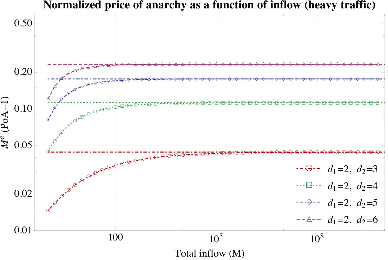 Figure 1
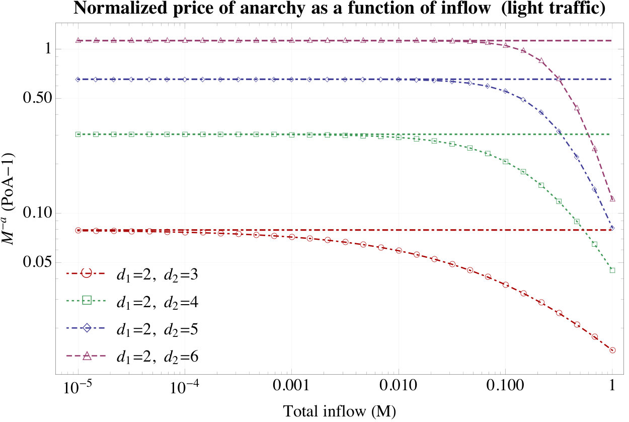 Figure 2
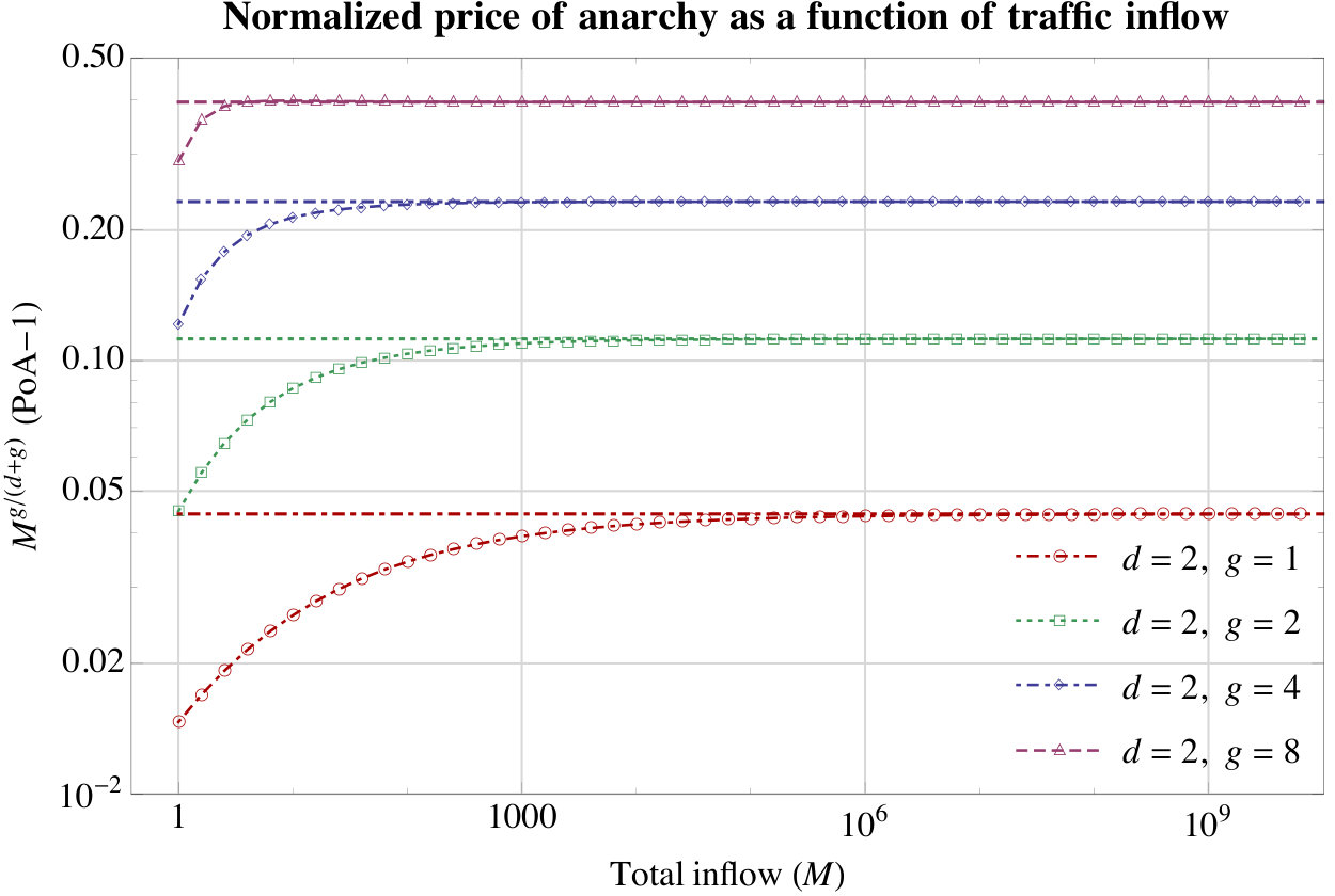 Figure 3
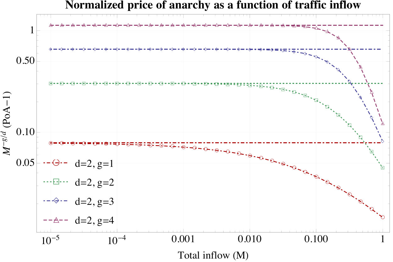 Figure 4
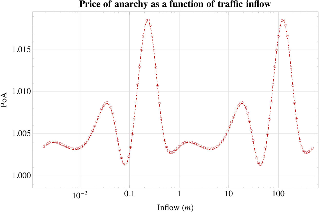 Figure 5
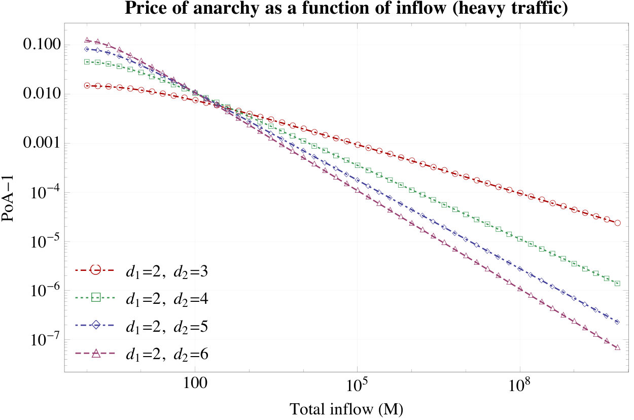 Figure 6
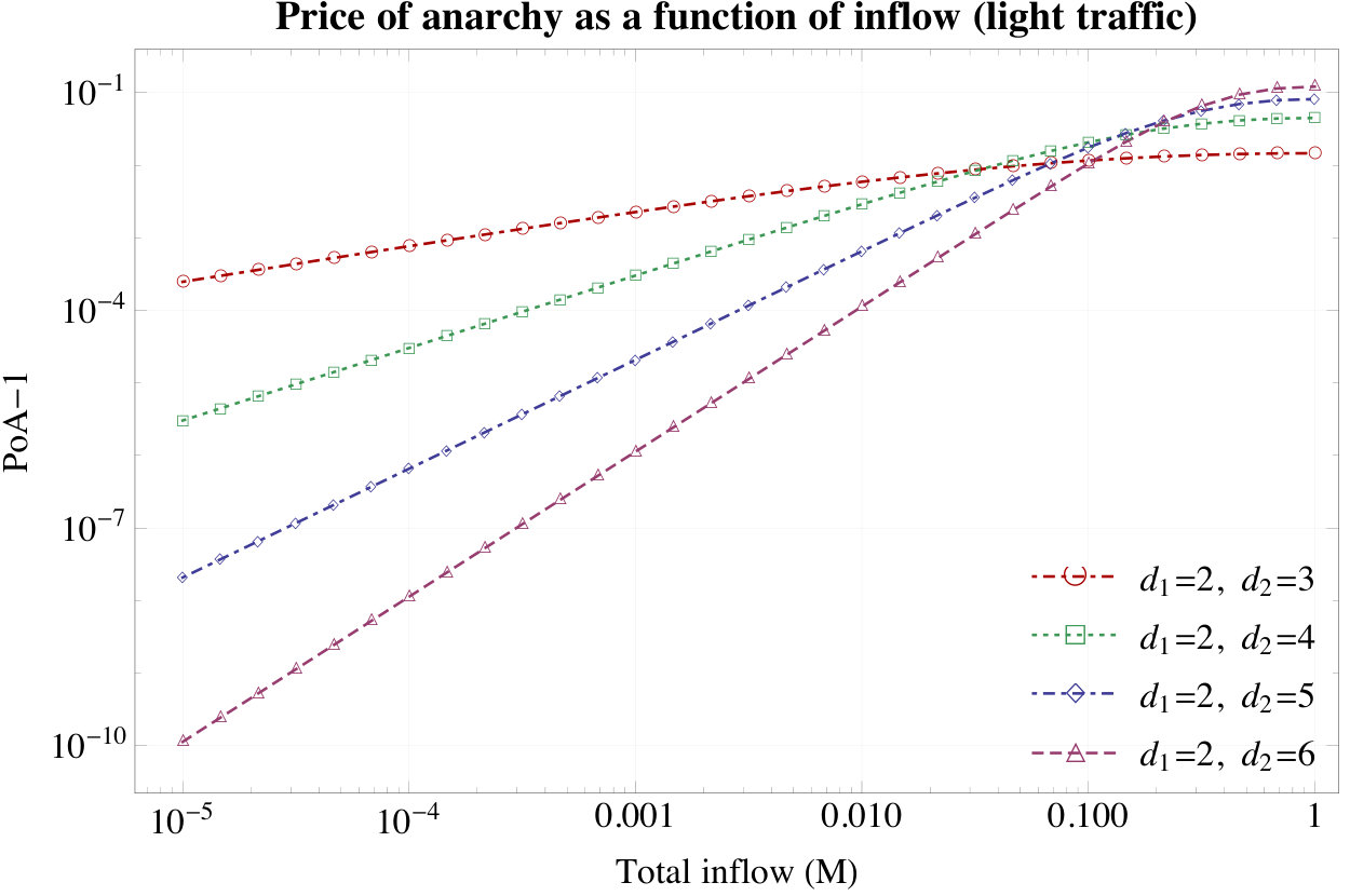 Figure 7
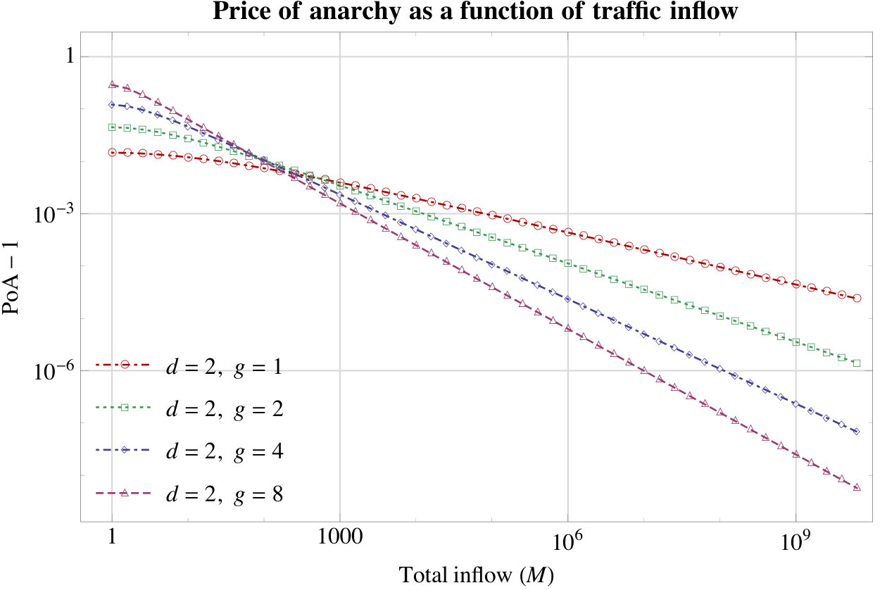 Figure 8
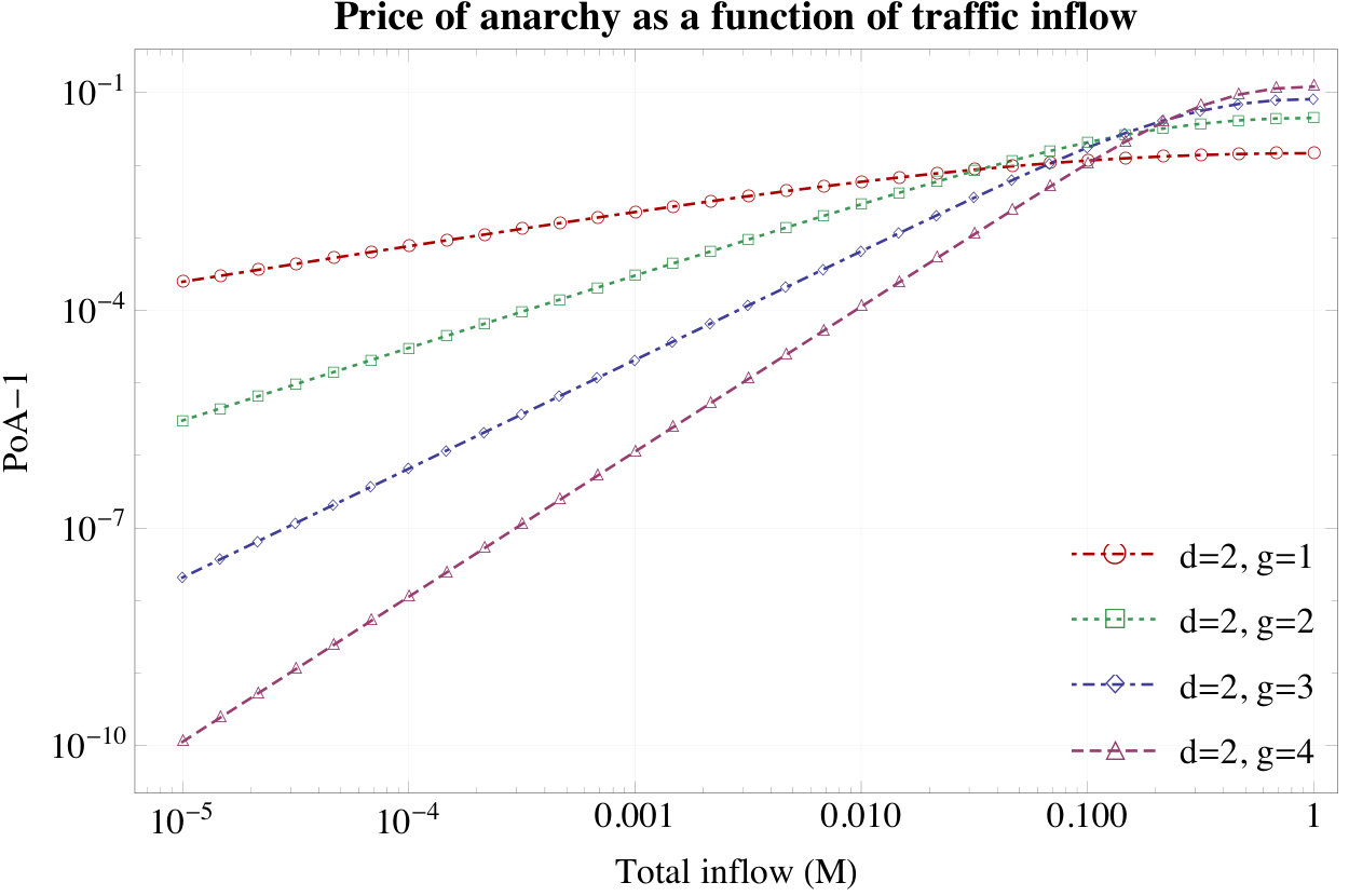 Figure 9
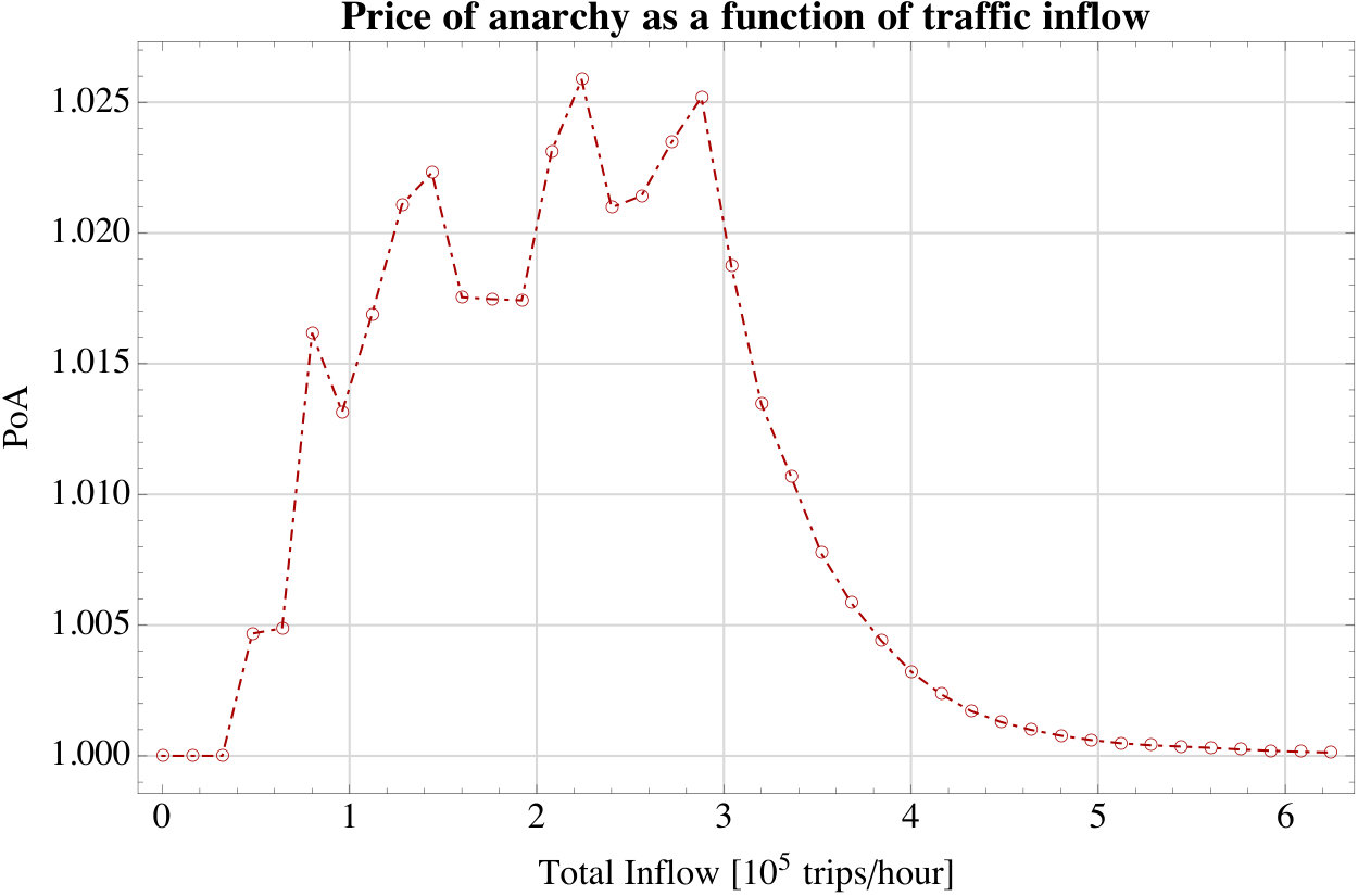 Figure 10
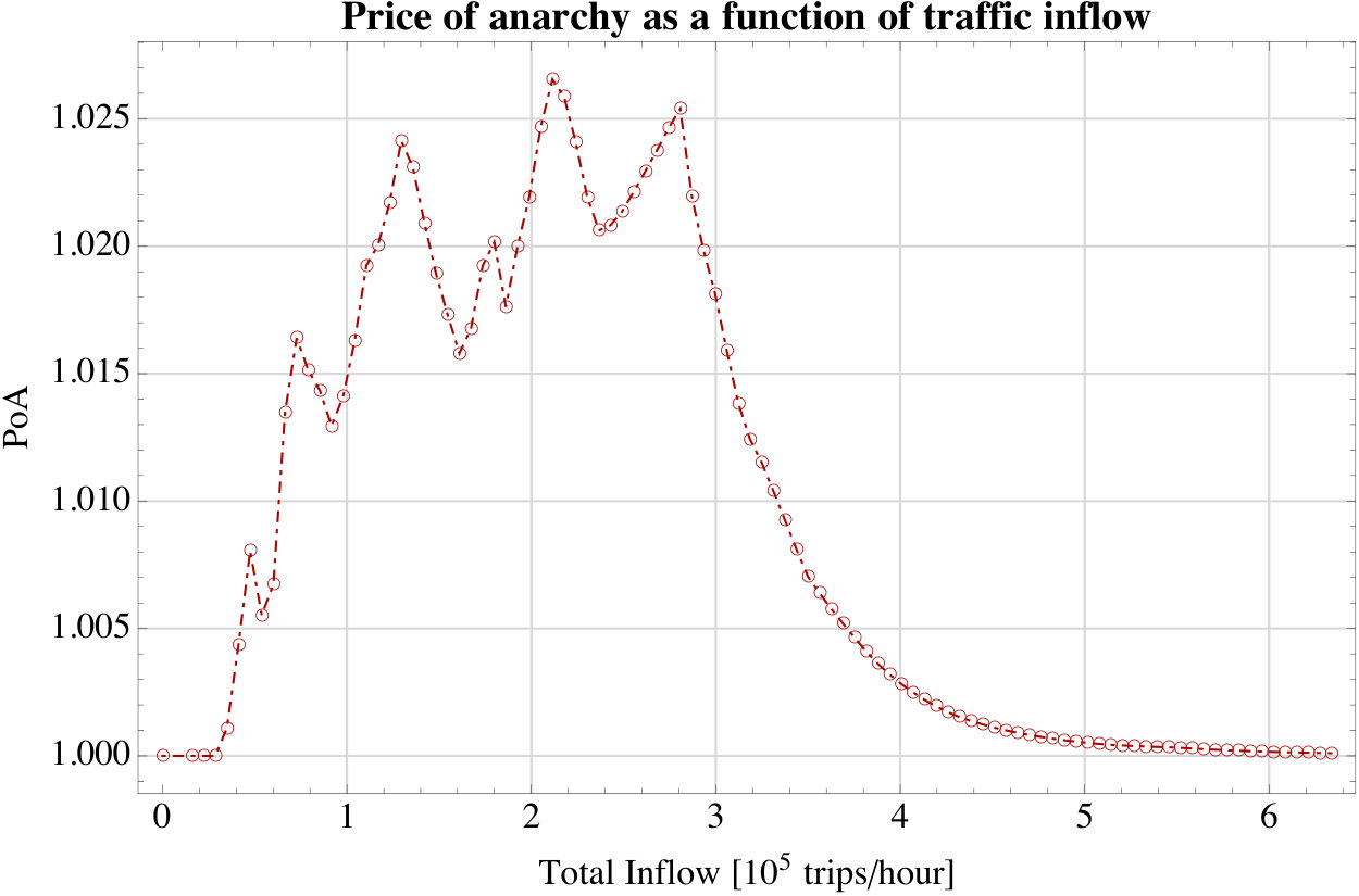 Figure 11
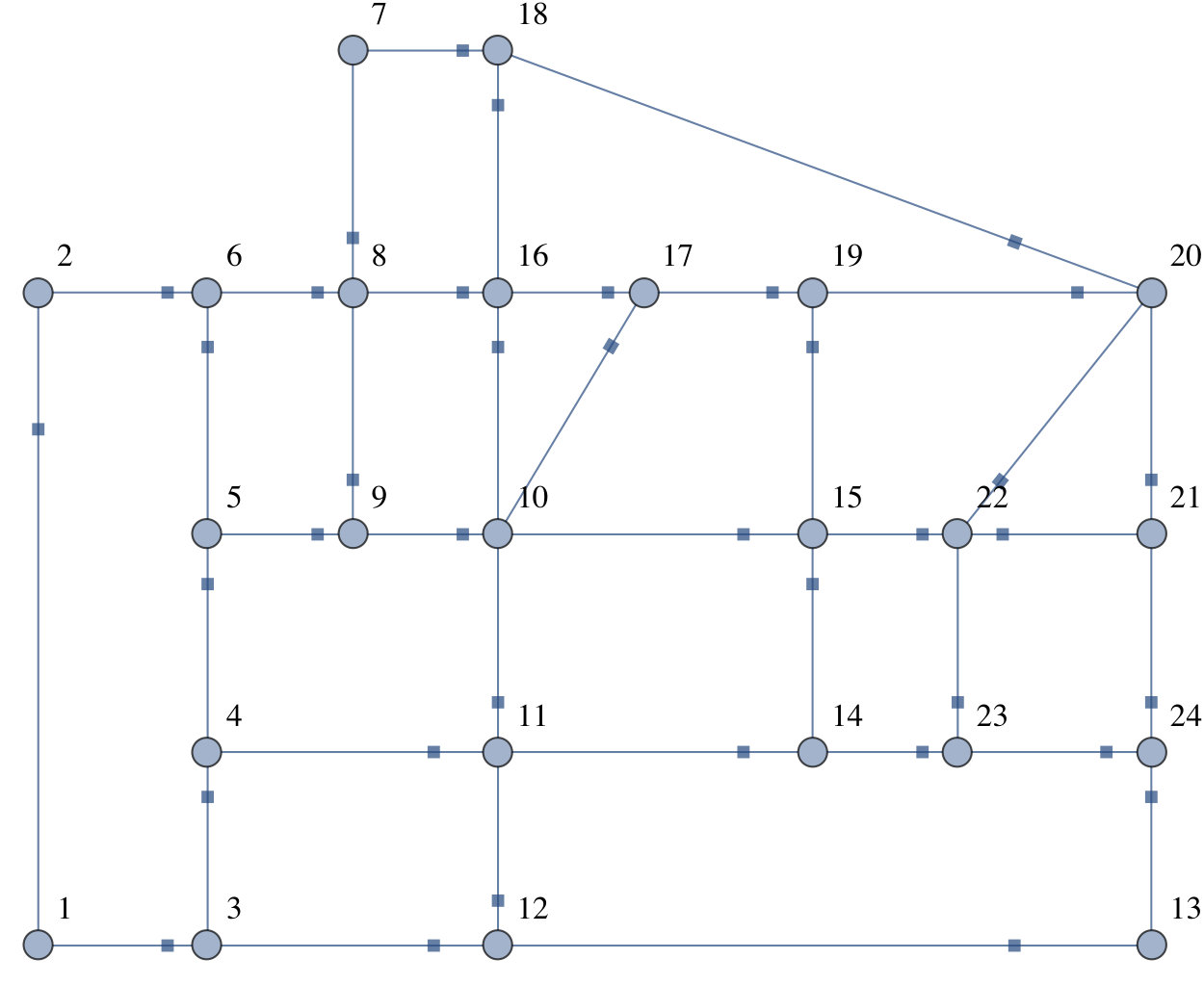 Figure 12
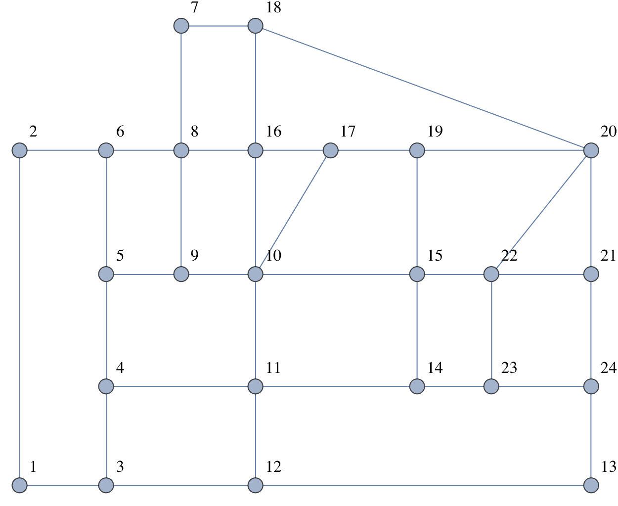 Figure 13
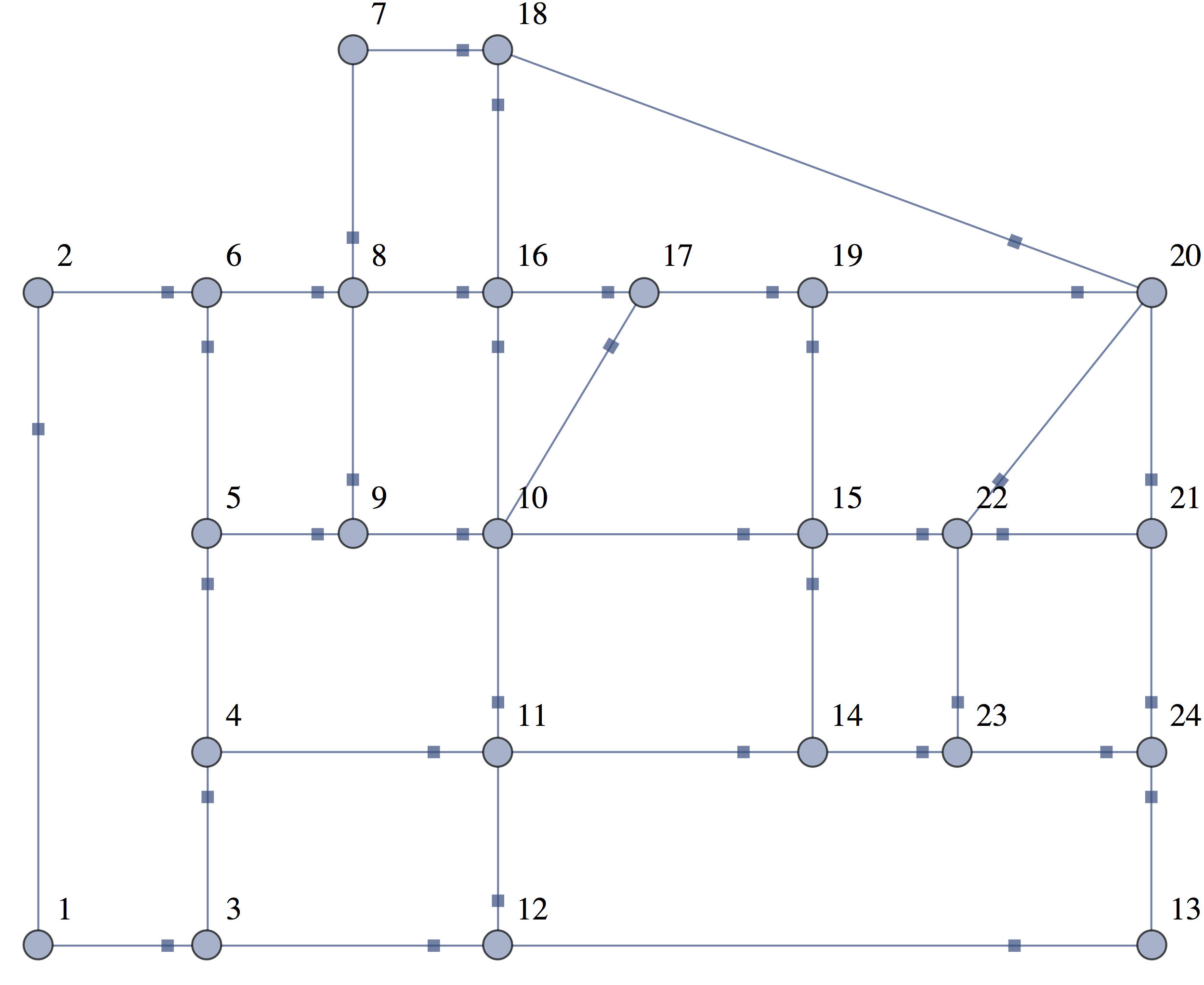 Figure 14
Peer Reviews
No public reviews on file for this paper yet. If you reviewed it on a platform where reviews are public (OpenReview, ICLR, NeurIPS, ICML), you can paste yours below so the community can read it here.
Videos
No videos yet. Explain this paper in a talk, walkthrough, or lecture? Add one.
When is selfish routing bad?
The price of anarchy in light and heavy traffic
Riccardo Colini-Baldeschi*∗*
∗ Core Data Science Group, Facebook Inc., 1 Rathbone Place, London, W1T 1FB, UK.
,
Roberto Cominetti*‡*
‡ Facultad de Ingeniería y Ciencias, Universidad Adolfo Ibáñez, Santiago, Chile.
,
Panayotis Mertikopoulos*§*
§ Univ. Grenoble Alpes, CNRS, Inria, LIG, F-38000 Grenoble, France.
and
Marco Scarsini*¶*
¶ Dipartimento di Economia e Finanza, LUISS, Viale Romania 32, 00197 Roma, Italy.
Abstract.
This paper examines the behavior of the price of anarchy as a function of the traffic inflow in nonatomic congestion games with multiple origin-destination (O/D) pairs. Empirical studies in real-world networks show that the price of anarchy is close to in both light and heavy traffic, thus raising the question: can these observations be justified theoretically? We first show that this is not always the case: the price of anarchy may remain a positive distance away from for all values of the traffic inflow, even in simple three-link networks with a single O/D pair and smooth, convex costs. On the other hand, for a large class of cost functions (including all polynomials), the price of anarchy does converge to in both heavy and light traffic, irrespective of the network topology and the number of O/D pairs in the network. We also examine the rate of convergence of the price of anarchy, and we show that it follows a power law whose degree can be computed explicitly when the network’s cost functions are polynomials.
Key words and phrases:
Nonatomic congestion games; price of anarchy; light traffic; heavy traffic; regular variation.
2010 Mathematics Subject Classification:
Primary 91A13; secondary 91A43, 91A80.
We thank an anonymous reviewer of an earlier conference version of this paper for suggesting one of the examples with variable inflows in Section 6.
This research benefited from the support of the FMJH Program PGMO under grant HEAVY.NET and from the support of EDF, Thales, and Orange. R. Colini-Baldeschi and M. Scarsini are members of GNAMPA-INdAM. R. Cominetti and P. Mertikopoulos gratefully acknowledge the support and hospitality of LUISS during a visit in which this research was initiated. R. Cominetti’s research is also supported by FONDECYT 1130564 and Núcleo Milenio ICM/FIC RC130003 “Información y Coordinación en Redes.” P. Mertikopoulos was partially supported by the ECOS/CONICYT Grant C15E03 and the Huawei HIRP Flagship project ULTRON. P. Mertikopoulos and M. Scarsini also gratefully acknowledge the support and hospitality of FONDECYT 1130564 and Núcleo Milenio “Información y Coordinación en Redes.”
“Traffic congestion is caused by vehicles, not by people in themselves.”
— Jane Jacobs, The Death and Life of Great American Cities
1. Introduction
Almost every commuter in a major metropolitan area has experienced the frustration of being stuck in traffic. At best, this might mean being late for dinner; at worst, it means more accidents and altercations, not to mention the vastly increased damage to the environment caused by huge numbers of idling engines.
To name but an infamous example, China’s G110 traffic jam in August 2010 brought to a standstill thousands of vehicles for 100 kilometers between Hebei and Inner Mongolia. The snarl-up lasted twelve days and resulted in drivers being unable to move for more than 1 kilometer per day, reportedly spending up to five days trapped in the jam. Not caused by weather or a natural disaster, this massive -day tie-up was instead laid at the feet of a bevy of trucks swarming on the shortest route to Beijing, thus clogging the highway to a halt (while ironically carrying supplies for construction work to ease congestion). This, therefore, raises the question: how much better would things have been if all traffic had been routed by a social planner who could calculate (and enforce) the optimum traffic assignment?
In game-theoretic terms, this question boils down to the inefficiency of Nash equilibria that are not Pareto optimal. The most widely used quantitative measure of this inefficiency is the so-called price of anarchy (PoA): introduced by *Koutsoupias and Papadimitriou, * (1999) and so dubbed by *Papadimitriou, * (2001), the price of anarchy is simply the ratio of the social cost of the least efficient Nash equilibrium divided by the minimum achievable social cost. By virtue of this straightforward definition, deriving worst-case bounds for the price of anarchy has given rise to a vigorous literature at the interface of operations research, economics and computer science, often leading to surprising and counter-intuitive results.
In the context of network congestion, *Pigou, * (1920) was probably the first to note the inefficiency of selfish routing, and his elementary two-road example with a price of anarchy (PoA) of is one of the two prototypical examples thereof. The other example is due to *Braess, * (1968), and consists of a four-road network where the addition of a zero-cost segment makes things just as bad as in the Pigou case. These two examples were the starting point for *Roughgarden and Tardos, * (2002) who showed that the price of anarchy in (nonatomic) routing games with affine costs may not exceed . On the other hand, if the network’s cost functions are polynomials of degree at most , the price of anarchy may become as high as , implying that selfish routing can become arbitrarily bad in networks with polynomial costs (*Roughgarden, *, 2003).
By this token, and given the typically nonlinear relation between traffic loads and travel times, the intervention of a central planner seems necessary in order to regain some degree of efficiency. At the same time however, these worst-case instances are typically realized in networks with delicately tuned traffic loads and costs: if a network operates beyond this regime, it is not clear whether the price of anarchy remains high. In view of this, our aim in this paper is to examine the asymptotic behavior of the price of anarchy at both ends of the congestion spectrum: light and heavy traffic.
Using both analytical and numerical methods, a very recent study by *O’Hare et al., * (2016) suggests that the price of anarchy is usually close to for both high and low traffic, and it fluctuates in the intermediate regime (typically exhibiting multiple local maxima). In a similar setting, *Monnot et al., * (2017) used a huge dataset on commuting students in Singapore to estimate the so-called “stress of catastrophe”: this majorant of the ordinary price of anarchy was estimated to a value between and , suggesting that the actual value of the price of anarchy in Singapore is lower (and definitely below the worst-case bound of the Pigou/Braess examples).
All this leads to the following natural questions:
- a)
Under what conditions does the price of anarchy converge to in light/heavy traffic? 2. b)
Do these conditions depend on the network topology, its cost functions, or both? 3. c)
Can general results be obtained for networks with multiple O/D pairs? 4. d)
When these conditions are satisfied, how fast is this convergence?
1.1. Our contributions
Our first result is a cautionary tale: we show that the price of anarchy may oscillate between two bounds strictly greater than for all values of the traffic inflow, even in simple parallel-link networks with a single O/D pair (cf. Fig. 1). The cost functions in our example are convex and differentiable, so neither convexity nor smoothness seem to play a major role in the efficiency of selfish routing. Moreover, our construction only involves a three-link network, so such phenomena may arise in any network containing such a three-link component.
Heuristically, the reason for this irregular – and, perhaps, counter-intuitive – behavior is that the growth rate of the network’s cost functions exhibits higher-order oscillations which persist at any scale, in both light and heavy traffic. To dispense with such pathologies, we focus on networks whose cost functions are asymptotically comparable to a benchmark function which is itself assumed to be regularly varying (cf. Definition 4.1). In so doing, we obtain a classification of the network’s edges, paths, and O/D pairs as fast, slow or tight relative to the chosen benchmark. Then, thanks to this classification, we obtain the following general result: If the routing cost of the “most costly” O/D pair in the network behaves like the benchmark, the network’s price of anarchy converges to in both light and heavy traffic.
Polynomial cost functions satisfy all of the above requirements, leading to the comprehensive asymptotic principle:
*In networks with polynomial costs,
the price of anarchy becomes under both light and heavy traffic.*
In other words, a benevolent social planner with full control of traffic assignment would not do any better than selfish agents in conditions of high or low congestion. In particular, only if the traffic falls in an intermediate regime can there be a substantial gap between optimum and equilibrium states.
To assess how wide this intermediate regime might be in practice, we also examine the speed at which the price of anarchy converges to as a function of the traffic inflow. Specializing to networks with polynomial costs, we find that in both regimes the convergence follows a power law with respect to the total traffic inflow, and we derive explicit sharp estimates for the corresponding rates.
1.2. Related work
Establishing worst-case bounds for the price of anarchy under different conditions has been a staple of the literature on congestion games ever since the seminal result of *Roughgarden and Tardos, * (2002). In words, this result states that in networks with affine costs the price of anarchy is no higher than , independently of the network topology and/or the number of O/D pairs in the network. Furthermore, this bound is sharp in that, for every , there exists a network with traffic inflow and affine costs such that the price of anarchy is exactly equal to . Importantly, our analysis shows that the order of the quantifiers in the above statement cannot be exchanged: in any network with affine costs, the price of anarchy gets arbitrarily close to if the traffic inflow is sufficiently large or small.
Worst-case bounds for the price of anarchy have been obtained for larger classes of cost functions. For polynomial costs with degree at most , *Roughgarden, * (2003) showed that the worst possible instance grows as while *Dumrauf and Gairing, * (2006) provided sharper bounds for monomials of maximum degree and minimum degree . Extending the above results, *Roughgarden and Tardos, * (2004) provided a unifying result for costs that are differentiable with convex, while *Correa et al., * (2004, 2008) considered less regular classes of cost functions. *Correa et al., * (2007) also studied the price of anarchy when the goal is to minimize the maximum – rather than the average – latency in the network. For a survey, the reader is referred to *Roughgarden, * (2007).
In a more practical setting, *Youn et al., * (2008) studied the difference between optimal and actual system performance in real transportation networks, focusing in particular on Boston’s road network. They observed that the price of anarchy depends crucially on the total traffic inflow: it starts at , it then grows with some oscillations, and ultimately returns to as the flow increases. *González Vayá et al., * (2015) studied optimal scheduling for the electricity demand of a fleet of plug-in electric vehicles: without using the term, they showed that the price of anarchy goes to as the number of vehicles grows. *Cole and Tao, * (2016) showed that in large Walrasian auctions and in large Fisher markets the price of anarchy goes to one as the market size increases. Finally, *Feldman et al., * (2016) took a different asymptotic approach and considered atomic games where the number of players grows to infinity. Applying the notion of -smoothness to the resulting sequence of atomic games, they showed that the price of anarchy converges to the corresponding nonatomic limit.
From an analytic standpoint, the closest antecedent to our paper is the recent work of *Colini-Baldeschi et al., * (2016) who studied the heavy traffic limit of the price of anarchy in parallel networks with a single O/D pair. Their analysis identified that regular variation plays an important role in this setting; however, it offered no insights into non-parallel networks with multiple O/D pairs or the light traffic regime. Our paper provides an in-depth answer to these questions: we show that
(a) regular variation yields asymptotic efficiency under both light and heavy traffic conditions;
(b) the topology of the network doesn’t matter; and
(c) the existence of several O/D pairs doesn’t matter as long as they admit a common benchmark (which is always the case if the network’s cost functions are polynomial).
Building on a previous unpublished version of the present paper, *Wu et al., * (2017) introduced a class of congestion games, called scalable, whose price of anarchy converges to as the total demand diverges. They also computed the rate of convergence of the price of anarchy for the special case of BPR cost functions of the same degree. *Stidham, * (2014) also studied the behavior of the price of anarchy for queueing networks in heavy traffic under various assumptions on the structure of the network and on the stochastic properties of the queues. His results can be used for the analysis of network routing models with capacity constraints.
Our work should also be compared to that of *Monnot et al., * (2017) who performed an empirical study of the price of anarchy based on data from thousands of commuting students in Singapore. Focusing on the network’s “stress of catastrophe” (an empirical majorant of the network’s price of anarchy), they showed that routing choices are near-optimal and the incurred price of anarchy is much lower than what traditional worst-case bounds suggest. Interestingly, the study of *Monnot et al., * (2017) also suggests that the Singapore road network is often lightly congested: as such, their results can be seen as a practical validation of the light traffic results presented here (and, conversely, our results provide a theoretical justification for their empirical observations).
1.3. Outline of the paper
The paper is organized as follows. In Section 2, we introduce the basic model and concepts that will be used in the rest of the paper. Section 3 provides two motivating examples for the analysis to follow. In Section 4, we treat networks with a single O/D pair, whereas Section 5 examines networks with multiple O/D pairs. The more complicated case of variable relative inflows is treated in Section 6. Finally, in Section 7, we study the rate of convergence of the price of anarchy in light and heavy traffic. To streamline our presentation, the proofs of our main results have been relegated to a series of appendices at the end of the paper.
2. Model and preliminaries
2.1. Network model
Following *Beckmann et al., * (1956) and *Roughgarden and Tardos, * (2002), the basic component of our model will be a directed multi-graph with vertex set and edge set (both finite). We further assume that there is a finite set of origin-destination (O/D) pairs indexed by , each with an individual traffic demand that is to be routed from the pair’s origin node to its destination . To route this traffic, the -th O/D pair employs a set of paths joining to , with each path comprising a sequence of edges that meet head-to-tail in the usual way; specifically, we do not assume that is necessarily the set of all paths joining to , but only some subset thereof. [This distinction is particularly relevant for packet-switched networks (such as the Internet) where only paths with a low hop count are typically employed.] For bookkeeping reasons, we will also make the following standing assumptions throughout our paper:
- a)
The total inflow rate is positive (so there is a nonzero amount of traffic in the network). 2. b)
The path sets are disjoint (which in particular holds trivially if all pairs are distinct).
Now, writing for the union of all such paths, the set of feasible routing flows in the network is defined as
[TABLE]
In turn, a routing flow induces a load on each edge as
[TABLE]
and we write for the corresponding load profile on the network. Given all this, the delay (or latency) experienced by an infinitesimal traffic element traversing edge is determined by a nondecreasing continuous cost function : more precisely, if is the load profile induced by a feasible routing flow , the incurred delay on edge is . Hence, with a slight abuse of notation, the associated cost of path will be given by
[TABLE]
Putting together all of the above, the tuple will be referred to as a (nonatomic) routing game. When we want to explicitly keep track of the total inflow rate , we write instead of ; also, when there is a single O/D pair, we will drop all reference to and altogether.
2.2. Equilibrium, optimality, and the price of anarchy
In routing games, the notion of Nash equilibrium is captured by Wardrop’s first principle: at equilibrium, the delays along utilized paths are equal and no higher than those that would be experienced by an infinitesimal traffic element going through an unused route (*Wardrop, *, 1952).
Formally, a routing flow is said to be a Wardrop equilibrium (WE) of if, for all , we have
[TABLE]
From the work of *Beckmann et al., * (1956), it is known that Wardrop equilibria coincide with the solutions of the (convex) minimization problem
[TABLE]
where denotes the primitive of . Analogously, socially optimum (SO) flows are defined as solutions of the total cost minimization problem
[TABLE]
By a simple rearrangement of terms, the objective function of (SO) can be rewritten as , so the value of the above problem can be expressed equivalently (and somewhat more concisely) as
[TABLE]
where denotes the set of all load profiles of the form (2.2). Thus, to quantify the gap between solutions to (WE) and (SO), let
[TABLE]
where is the load profile induced by a Wardrop equilibrium of (by a standard result of *Beckmann et al., * (1956), all such flows incur the same total cost). The game’s price of anarchy (PoA) is then defined as
[TABLE]
For this ratio to be well-defined, we must have ; otherwise, if this is not the case, we will vacuously set . To avoid such technicalities, we will tacitly assume that throughout.
Of course, with equality if and only if Wardrop equilibria are also socially efficient. Our main objective in what follows will be to study the asymptotic behavior of this ratio when or .
3. First results
3.1. Sioux Falls: a representative case study
To motivate our analysis, we begin by examining the behavior of the price of anarchy in the road network of Sioux Falls, a standard case study in the transportation literature. For concreteness, the network’s (two-way) arterial roads are shown in Fig. 2(a) and their delay functions are taken to be of the BPR (Bureau of Public Roads) type
[TABLE]
with coefficients and degrees (typically ) taken from the standard reference work of *LeBlanc et al., * (1975, Table 1). To analyze the network’s price of anarchy as a function of the total traffic inflow, we considered all O/D pairs with nonzero inflow, and for each O/D pair , we restricted to contain only the five shortest paths in terms of free-flow travel time (i.e., the time taken to traverse a path when empty). We then scaled up or down these inflows preserving the ratios between different O/D pairs and we plotted the network’s price of anarchy for various values of the total inflow .
As can be seen from Fig. 2(b), the network’s price of anarchy is identically equal to when the total inflow is small enough (approximately up to trips per hour); for intermediate values of , the price of anarchy becomes strictly greater than , and, ultimately, it decreases monotonically to in the heavy traffic limit. Interestingly, *LeBlanc et al., * (1975) report a value of for the network’s median traffic inflow; this value is well within the range where the price of anarchy decreases monotonically to and, indeed, the observed value is approximately equal to , indicating a difference between socially optimum and equilibrium flows under median traffic conditions.
Similar conclusions have been drawn in the literature from empirical studies in London, New York and Boston (*Youn et al., *, 2008), as well as Sioux Falls with different subsets of O/D pairs and connecting paths per pair (*O’Hare et al., *, 2016). In particular, in all cases, it was observed that there is an initial interval of values of for which the price of anarchy is identically equal to ; our first result shows that this is not mere happenstance:
Proposition 3.1**.**
If the network’s cost functions are of the form (3.1) with and for all , we have for all sufficiently small .
In fact, as the following result shows, this behavior arises whenever each O/D pair admits a single “best” path under zero inflow:
Proposition 3.2**.**
Let denote the set of minimal cost paths of the -th O/D pair under zero inflow. If is a singleton for all , we have for all sufficiently small .
The above results (both proven in Appendix A) provide a reasonable theoretical justification for the light traffic behavior of the price of anarchy that is observed in Fig. 2 (the heavy traffic limit is discussed in detail in the next sections). At the same time however, the BPR and “unique best path” assumptions in Propositions 3.1 and 3.2 respectively suggest that there is a finer mechanism at play which becomes apparent when the total cost at low traffic depends more delicately on the distribution of traffic in the network. We make this precise in the following section where we provide an example of a three-link network where the price of anarchy oscillates between two values strictly greater than , for all values of the traffic inflow.
3.2. A network where selfish routing is always inefficient
To construct an example of an “always inefficient” network, our approach will be to take a network with a certain degree of periodicity, obtain an explicit handle for its price of anarchy over a compact interval, and then tessellate this behavior over the entire traffic spectrum . To carry this out, let be a nonatomic routing game consisting of a single O/D pair with traffic inflow . This traffic is to be routed over the three-link parallel graph of Fig. 1 with cost functions
[TABLE]
where is a positive integer. It is easy to see that these cost functions are increasing, strictly convex and smooth on for all , and they all grow as at both traffic limits ( and ). Furthermore, the functions are strictly convex, so the optimum traffic allocation problem (SO) admits a unique solution. Hence, the only way for the game’s price of anarchy to be equal to is when the game’s (also unique) Wardrop equilibrium coincides with the network’s socially optimum flow.
As we show in Appendix A, the equations determining the network’s equilibrium and optimum flows never admit a common solution, so the price of anarchy is strictly greater than over any compact interval (showing in this way that the conclusion of Propositions 3.1 and 3.2 already fails for this example). Moreover, the trigonometric terms in (3.2) imply that these equations are periodic in a logarithmic scale (i.e., in ). Hence, combining these two properties, we obtain:
Proposition 3.3**.**
In the three-link parallel network defined above, is periodic in and oscillates between two values strictly greater than .
*Colini-Baldeschi et al., * (2016) already provided examples of networks where but the cost functions involved were fairly irregular and the of the price of anarchy was still (i.e., selfish routing was still efficient infinitely often). By contrast, in the above example, the price of anarchy is bounded away from for all possible demands, and this despite the fact that the network’s cost functions are smooth, strictly convex and grow as at both ends of the congestion spectrum. This is a considerable sharpening of the example of *Colini-Baldeschi et al., * (2016) as it shows that there are cases where efficiency is never achieved at equilibrium – not even asymptotically.
4. Networks with a single O/D pair
Despite the highly smooth and convex structure of the example network of Proposition 3.3, closer inspection reveals that the growth rate of its cost functions exhibits persistent oscillations at both [math] and . This naturally leads to the following question: Does selfish routing remain bad for “reasonable” cost functions that do not behave irregularly in the limit?
To quantify – and discard – such irregularities, we will employ the seminal notion of regular variation (recalled below). For clarity and concision, we will focus for now on networks with a single O/D pair; the case of multiple O/D pairs will be discussed in detail later, in Sections 5 and 6.
4.1. Regular variation and edge classification
To present a unified perspective, we will tackle both ends of the congestion spectrum simultaneously by introducing the traffic limit indicator : letting gives the light traffic limit for and the heavy traffic limit for . Regular variation at either limit is then defined as follows:
Definition 4.1**.**
A function is said to be regularly varying at if
[TABLE]
In words, regular variation means that grows at the same rate when viewed at different scales (determined here by ). The concept itself dates back to *Karamata, * (1930, 1933) and has been used extensively in functional analysis, probability, and large deviations theory (see e.g., *de Haan and Ferreira, *, 2006; *Jessen and Mikosch, *, 2006; *Resnick, *, 2007); for a comprehensive survey we refer the reader to *Bingham et al., * (1989).
Standard examples of regularly varying functions include all affine functions, polynomials, logarithms, and, more generally, all analytic functions (barring those with an essential singularity at ). [Recall here that a function is analytic on a domain if it is equal to its Taylor series on .] On the other hand, despite being bounded from above and below as , the oscillatory cost functions (3.2) used in the counterexample of Section 3 are not regularly varying. Indeed, at either or , the limit
[TABLE]
does not exist in unless for some (and likewise for ). In this way, regular variation provides a much finer view than polynomial growth.
With all this at hand, we will dispose of growth irregularities like the above by positing that the network’s cost functions can be compared asymptotically to some regularly varying function . Specifically, given an ensemble of cost functions , we will say that a regularly varying function is a benchmark for at if the following (possibly infinite) limit exists for all
[TABLE]
This limit will be called the index of edge at , and will be called fast, slow, or tight (relative to at ) if is respectively [math], , or in-between. In particular, when is tight, is also regularly varying and exhibits the same asymptotic behavior as the benchmark function at ; if is fast, then ; and, finally, if is slow, then . As such, a benchmark function groups the network’s edges into three equivalence classes that exhibit the same qualitative behavior with respect to .
Of course, this partition depends on the chosen benchmark and the traffic limit (light or heavy): for instance, is fast with respect to at [math], but it is slow at . For concision, we will not keep track of this dependence explicitly and instead rely on the context to resolve any ambiguities. However, it will be important to keep in mind that the classification of fast and slow edges could be flipped when transitioning from heavy to light traffic and vice versa.
Now, since bottlenecks along a path are caused by its slowest edges, we also define the index of a path as
[TABLE]
and we say that is fast, slow, or tight based on whether is [math], , or in-between. Finally, given that traffic will tend to be routed along the fastest paths in the network, we define the index of the network as
[TABLE]
and we say that the network is itself tight if . In words, a path is fast (resp. tight/slow) if its slowest edge is fast (resp. tight/slow), and a network is tight if its fastest path is tight.
Defined this way, tightness guarantees that the network admits a path whose cost behaves asymptotically as a (positive) multiple of the benchmark function . The importance of this requirement is again illustrated by the cost model (3.2) of the previous section: if we only assumed that the network admits a path whose cost behaves as , then we would not be able to rule out the pathological oscillations of the example in Section 3.
4.2. The light traffic limit
Thanks to the above legwork, we are in a position to state our main result for lightly congested networks with a single O/D pair:
Theorem 4.2**.**
Let be a nonatomic routing game with a single O/D pair. If the network is tight under light traffic (), then
[TABLE]
In words, Theorem 4.2 simply states that if the cost of the network’s fastest path is regularly varying at [math], selfish routing becomes efficient in light traffic. To streamline our presentation, Theorem 4.2 is proved in Appendix B as a special case of a much more general statement. Here, we focus on some immediate corollaries thereof:
Corollary 4.3**.**
Suppose that, for every edge , the limit is finite and nonzero for some . Then, as .
Proof.
Referring to as the order of , define the order of a path as and that of the network as . Clearly, if and only if ; if and only if ; and if and only if . This shows that the network is tight with respect to at [math], so Theorem 4.2 applies. ∎
Corollary 4.4**.**
In a single O/D-network with analytic costs we have as .
Proof.
If for small enough , we have for . Our claim then follows from Corollary 4.3. ∎
Corollary 4.5**.**
In a single O/D-network with polynomial costs we have as .
Of the above results, Corollaries 4.4 and 4.5 are of special practical interest because most latency models that have been proposed in the literature are polynomial or analytic at [math]. In urban networks, the golden standard is the Bureau of Public Roads (BPR) quartic model , while basically all of the established queueing models used in the theory of packet-switched networks (, , , etc.) are analytic at [math] (*Bertsekas and Gallager, *, 1992).
Despite appearances, the very wide applicability of Theorem 4.2 and its corollaries is fairly surprising. Indeed, at first sight, one would expect that when , traffic is so light that it doesn’t really matter how it is routed. This is indeed the case if, for instance, all paths in the network exhibit different positive costs when (cf. Proposition 3.2). However, if the cost of an empty path is zero, this is no longer the case: the optimum and equilibrium traffic assignments could be fairly different (even when the network is lightly congested), so there is no a priori reason for the price of anarchy to converge to as (the example of Section 3 clearly illustrates this phenomenon). Theorem 4.2 shows that all that is needed for this to occur is for the network’s cost functions to be faithfully represented by a common benchmark function: when this condition is met, optimum and equilibrium costs no longer fluctuate but, instead, they converge to the same value.
4.3. The heavy traffic limit
Our main result for highly congested networks with a single O/D pair is as follows:
Theorem 4.6**.**
Let be a nonatomic routing game with a single O/D pair. If the network is tight under heavy traffic (), then
[TABLE]
In words, Theorem 4.6 simply states that if the cost of the network’s fastest path is regularly varying at , selfish routing becomes efficient in heavy traffic. To compare and contrast the light and heavy traffic regimes, we relegate the proof of Theorem 4.6 to Appendix B and only focus here on some immediate corollaries thereof:
Corollary 4.7**.**
Suppose there exists a path with bounded costs, that is, for all . Then, as .
Proof.
Taking , we get for all . By assumption, there exists a path such that , so Theorem 4.6 applies. ∎
Corollary 4.8**.**
Suppose that the limit is finite and nonzero for some and all . Then, as .
Proof.
Shadowing the proof of Corollary 4.3, let and (but note the reversal of the and operators). Clearly, if and only if ; if and only if ; finally, if and only if . This shows that the network is tight with respect to at , so Theorem 4.6 applies. ∎
Corollary 4.9**.**
In a single O/D-network with polynomial costs we have as .
In a certain, precise sense, Theorems 4.2 and 4.6 show that the high and low congestion regimes can be seen as different sides of the same coin. By excluding pathological oscillations at either end of the congestion spectrum, regular variation ensures asymptotic regularity and guarantees that selfish routing becomes efficient in the limit: specifically, tightness at [math] guarantees efficiency in light traffic while tightness at guarantees efficiency in heavy traffic. By this token, taking Corollaries 4.5 and 4.9 in tandem implies that selfish routing becomes efficient under both light and heavy traffic in networks with polynomial costs and a single O/D pair.
That being said, there are still important, quantitative differences between the light and heavy traffic limits. For instance, even though Corollaries 4.8 and 4.9 are direct analogues of their light traffic counterparts, the conclusion of Corollary 4.7 is false in light traffic (the three-link network of Section 3 serves again as a counterexample). In fact, even in the case of polynomial costs (Corollary 4.5 vs. Corollary 4.9), there is an important reversal of roles that takes place between fast and slow edges. Specifically, edges that are fast in light traffic typically become slow under heavy traffic and vice versa (importantly however, tight edges are not re-classified under this regime change). Nevertheless, despite this reversal, the price of anarchy still goes to in both cases.
5. Networks with multiple O/D pairs
We now extend our analysis to networks with multiple O/D pairs. In this case, if the inflow rate of the -th O/D pair is , the total traffic inflow in the network is given by
[TABLE]
and we write
[TABLE]
for the relative inflow rate of the -th O/D pair – i.e., the fraction of the total traffic generated by the pair in question. In the rest of this section, we will assume that the relative inflow of every O/D pair is a fixed positive constant that does not depend on ; the case of variable inflow rates will be discussed in detail in Section 6.
The key difference with the single-pair setting is that routing costs for different O/D pairs may exhibit completely different asymptotic behaviors in the limit. As a result, in the presence of multiple O/D pairs, the definition of the network’s index (and the related notion of tightness) must be re-examined. To do so, given that the traffic generated by an O/D pair will tend to be routed along the pair’s fastest path, we first define the index of an O/D pair as
[TABLE]
Just like edges and paths, this index can be used to classify O/D pairs as fast, slow or tight depending on whether is respectively [math], , or in-between. The index of the network is then defined as
[TABLE]
and we say that the network is tight if . Heuristically, this definition simply captures the fact that the leading contribution to congestion is due to the “costliest” O/D pairs in the network; obviously, if there is but a single O/D pair, this last point is moot and (5.4) reduces to (4.5).
Example 5.1*.*
To illustrate the above concepts, consider a Wheatstone network with two O/D pairs and cost functions as in Fig. 3. Focusing first on the heavy traffic limit, the benchmark would classify edge as tight, edges and as slow, and edges and as fast. Accordingly, the first O/D pair would be classified as tight while the second O/D pair would be classified as fast; since no pair is slow and at least one pair is not fast, the network is itself tight.
In the light traffic limit, the same benchmark would classify edges and as tight, edges and as slow, and edge as fast. Under this classification, the first O/D pair would again be tight, but the second O/D pair would now be classified as slow (because all its paths contain a slow edge), so the network would no longer be tight. A moment’s reflection shows that the reason for this is that the benchmark function is not well-suited for the second O/D pair. Instead, if we take the benchmark , the first O/D pair would be classified as fast (because it has a fast path, namely edge ) and the second pair would be classified as tight, so the network would now be tight. For a systematized version of this benchmark selection procedure, see the proof of Corollary 5.2 below.
With all this at hand, our next result states that if the costliest O/D pair in the network admits a tight path, selfish routing becomes asymptotically efficient in the limit:
Theorem 5.1**.**
Let be a nonatomic routing game. If the network is tight in the limit as , then
[TABLE]
In words, if
(a) every O/D pair has a path which is not slow, and
(b) the fastest path of the slowest O/D pair has a regularly varying cost,
selfish routing becomes efficient in the limit. Motivated by the strong connection between Theorems 4.2 and 4.6, Theorem 5.1 has been stated in a way that does not discriminate between the light and heavy traffic regimes. The reason for this is to highlight the role of the tightness assumption: tightness at [math] guarantees efficiency in light traffic () while tightness at guarantees efficiency in heavy traffic ().
Of course, both Theorems 4.2 and 4.6 follow as corollaries of Theorem 5.1 by taking respectively or and specializing to a single O/D pair (in which case Eqs. 4.5 and 5.4 coincide). Other than that, however, the same caveats apply regarding the passage from light to heavy traffic: the classification of fast and slow edges could be reversed, the equilibrium/socially optimum flows could be drastically different in the two regimes, etc. To illustrate all this, we proceed with some further corollaries of Theorem 5.1 (which we prove in Appendix B):
Corollary 5.2**.**
If the network’s costs are regularly varying at and the (possibly infinite) limit
[TABLE]
exists for all , then as .
Proof.
Define a total preorder among the network’s edges by setting if and only if . For each path , choose a maximal element of , i.e., an edge such that for all . Then, for each O/D pair , choose a path for which is minimal, i.e., for all . Finally, pick an O/D pair such that is maximal, i.e., for all . Setting and taking as a benchmark, it is easy to verify that the network is tight at , so Theorem 5.1 applies. ∎
The proof of Corollary 5.2 shows that the “comparison index” induces a preference relation which refines the coarser classification of the network’s edges into fast, slow and tight. Of course, this ordering could be reversed when passing from light to heavy traffic, but the existence thereof (along with regular variation) guarantees that the price of anarchy is asymptotically equal to in both cases.
In addition to the above, Corollary 5.2 also gives an alternative way to prove the following analogue of Corollaries 4.3 and 4.8:
Corollary 5.3**.**
Suppose that the limit is finite and nonzero for some and all . Then, as .
Proof.
Observe that
[TABLE]
so exists for all . Our claim then follows from Corollary 5.2. ∎
We thus obtain the following important corollary for polynomial cost functions:
Corollary 5.4**.**
In networks with polynomial costs, as .
In words, Corollary 5.4 yields the general principle that we stated in the introduction:
*In networks with polynomial costs,
the price of anarchy becomes under both light and heavy traffic.*
We find this principle particularly appealing as it indicates that the price of anarchy may attain high values only in an intermediate regime (where the traffic is neither light nor heavy).
6. Networks with variable inflow rates
An important assumption in the analysis of the previous section is that the relative inflow rate of each O/D pair does not fluctuate in the limit – i.e., all pairs are assumed to generate a constant fraction of the overall traffic. In general however, this assumption need not hold: for instance, in an urban road network, central O/D pairs generate disproportionately more traffic during rush hour than peripheral, suburban destinations, so it is not reasonable to assume that traffic scales up maintaining a constant traffic ratio between different O/D pairs.
To understand the impact of this variability, consider two independent links, and , with corresponding cost functions and . Suppose further that these links are joining two uncoupled O/D pairs with inflow rates and and total inflow . If both inflows scale in the limit as , the cost of the first pair will scale as while that of the second pair will scale as . As such, the leading contribution to congestion will be that of the first O/D pair in light traffic, and that of the second pair in heavy traffic. If, however, the inflow of the first pair scales as but that of the second pair scales as , the induced costs will scale respectively as and ; consequently, the most costly O/D pair will now be the second one in light traffic and the first one in heavy traffic.
This reversal of roles shows that the asymptotic behavior of the relative inflow rates could end up painting a completely different picture in the limit. In particular, if these relative rates oscillate wildly in the limit, the price of anarchy may exhibit a likewise irregular asymptotic behavior, even if the underlying network is well-behaved (for instance, even if it is tight; cf. Example 6.2 below). As a result, special care must be taken to define and study the asymptotic regime in networks with variable traffic demands.
To that end, let be a sequence of nonatomic routing games with total inflow induced by a sequence of inflow rates for each O/D pair . The light and heavy traffic limits are obviously recovered depending on whether the total inflow converges respectively to or as . However, the relative inflow rates could now exhibit very different behaviors as : in particular, as discussed above, the relative inflow of an O/D pair could oscillate – or even vanish – in the limit. To capture such phenomena, we introduce below the notion of salience:
Definition 6.1**.**
Let be a sequence of nonatomic routing games with relative inflow rates , . We say that a subset of O/D pairs is salient if
[TABLE]
i.e., if the total fraction of the traffic generated by the O/D pairs in is non-negligible in the limit.
Obviously, if the sequence of relative inflow vectors converges to a well-defined limit, will be salient if and only if some O/D pair of is itself salient – i.e., if and only if for some . However, if this is not the case, a set of O/D pairs may be salient even if none of its constituent pairs is salient: for instance, if there are two O/D pairs, “” and “”, with relative inflows , neither pair is salient but their union is (since for all ). Thus, the notion of salience does not rule out fluctuations in the relative inflows of individual O/D pairs; it only posits that the set of O/D pairs in question carries enough traffic in the limit.
Bearing all this in mind, our main result for networks with variable inflow rates is as follows:
Theorem 6.2**.**
Let be a sequence of nonatomic routing games with inflow rates and total inflow . Suppose further that:
- (a)
Traffic is either light or heavy in the limit, i.e., . 2. (b)
Every O/D pair has a path which is not slow, i.e., for all . 3. (c)
The set of tight O/D pairs is salient, i.e., .
Then, as .
Heuristically, Condition (a)* above simply indicates the traffic regime under study (light or heavy), whereas Condition (b) guarantees that the network’s benchmark function correctly classifies the paths that are not too costly in each O/D pair. Finally, Condition (c) guarantees that tight O/D pairs are indeed relevant in terms of traffic, i.e., they account for a non-negligible fraction of the total inflow.*
In view of all this, Theorem 6.2 can be seen as a direct extension of our “fixed-rate” analysis in Sections 4 and 5: indeed, in the case of constant (positive) relative inflows, salience boils down to asking that the network admits at least one tight O/D pair, so Theorem 5.1 can be obtained as a special case of Theorem 6.2. Below, we provide some further corollaries of Theorem 6.2 along these lines:
Corollary 6.3**.**
If every O/D pair in the network is tight, then .
Corollary 6.4**.**
If the network is tight and every O/D pair is salient, then .
On the other hand, it is worth noting that if salience fails, we can draw no definitive conclusions for the price of anarchy. We illustrate the main reasons for this via two examples below:
Example 6.1* (Efficiency without salience).*
Consider the simple network of Fig. 4, where two “uncoupled” O/D pairs respectively encounter a standard Pigou network and an independent link with zero cost. In heavy traffic, the benchmark function classifies the O/D pair as tight and the pair as fast, so the network is itself tight. Note also that the second O/D pair does not affect the network’s price of anarchy because it has a single routing option and its cost is identically equal to [math]; however, it still affects the definition of relative inflows.
If we take the inflow sequence and , we get and as , so the first O/D pair is not salient. Since the second O/D pair is not tight, Condition (c)* fails; nevertheless, if we apply Theorem 4.6 to the first O/D pair by itself, we obtain (recall here that the second pair does not affect the network’s PoA). In other words, Condition (c) is not necessary for selfish routing to be asymptotically efficient.*
Example 6.2* (Inefficiency without salience).*
Consider the same network as above but take the periodically oscillating inflow sequence
[TABLE]
We then have and so, again, Condition (c)* fails (but in a different way). This time, whenever is odd, the network’s price of anarchy is equal to that of a Pigou network with inflow (because the second O/D pair is costless). Thus, for odd, we get , which is the worst-case value for networks with affine costs; as such, the conclusion of Theorem 6.2 does not hold in general if we just drop the salience condition.*
The above examples suggest that there is a finer mechanism at work which is not captured by the intersection of tightness and salience. At a high level, the crucial component of this mechanism seems to be that asymptotic efficiency is guaranteed if the network remains tight after suitably modifying the network’s cost functions to take into account the scaling of the inflow of each O/D pair. However, getting an exact statement at this level of generality is fairly cumbersome, so we do not attempt it here.
7. Rate of convergence
The analysis of the previous sections provides a wide range of sufficient conditions guaranteeing that selfish routing becomes efficient in the limit; however, it does not provide any indication for the rate at which the network’s price of anarchy converges to . In this section, we derive such rates (including subleading terms) for networks with polynomial costs of the form
[TABLE]
where all coefficients are assumed nonnegative () and and respectively denote the smallest and largest powers present (so ); by convention, we also take and when . [This follows the standard – if somewhat surprising at first – convention that , .] This model covers in particular the BPR “constant plus monomial” model (3.1) but also extends more easily to networks with more intricate cost functions.
In contrast to our qualitative analysis, the two traffic limits (light and heavy) exhibit different quantitative behaviors, so we treat them separately.
7.1. The light traffic case
We begin with the light traffic limit (). To motivate our analysis, we start with a simple example of a Pigou network with monomial costs as shown in Fig. 5: for , the zero-flow travel time of both links is zero, so Proposition 3.2 does not apply. Instead, as we show below, the network’s price of anarchy decays to following a power law:
Proposition 7.1**.**
Consider a two-link parallel network with cost functions and , , and a single O/D pair with inflow . Then
[TABLE]
where
[TABLE]
In words, Proposition 7.1 shows that the rate of convergence of the price of anarchy is controlled by the ratio : the largest the ratio of degrees, the fastest the decay of the price of anarchy (for a numerical illustration, see Fig. 6). This behavior is consistent with Proposition 3.2 which predicts that if is small enough and . Indeed, taking in (7.2) shows that for any , suggesting in turn that the rate of decay of is qualitatively different in this case.
Another case worth noting is when , i.e., when both links are equivalent in terms of performance. In this case, is identically equal to for all values of (Proposition 3.1 already guarantees as much when is not large). However, (7.2) would seem to suggest that the price of anarchy can remain large as (since when ). The solution of this apparent paradox is provided by looking at the multiplicative constant : when , we also have , so the resulting contribution to the price of anarchy is [math] – not .
The above highlights the importance of the relative rate of decay of the network’s edge costs as a function of the inflow. Since monomials with lower exponents are more costly in the low traffic limit, this rate is dominated by the smallest power in (7.1). Thus, motivated by the index machinery of Sections 4 and 5, we respectively define the order of an edge , that of a path , of an O/D pair , and that of the network itself as
[TABLE]
In view of the above, the network is tight with respect to the benchmark function , and an edge is fast when , tight when , and slow if . We then denote the set of the network’s slow edges as
[TABLE]
for the order of the fastest edge in (again employing the standard convention that , so when there are no slow edges).
Building on the intuition gained from Proposition 7.1, our main quantitative result for low traffic is that the network’s PoA decays to following a power law that depends only on the ratio between the order of the network () and that of its fastest slow edge ():
Theorem 7.2**.**
Let be a nonatomic routing game with polynomial costs, total inflow , and fixed relative inflows. Then, there exist non-negative constants and such that
[TABLE]
where and whenever .
Theorem 7.2* was stated for networks with fixed relative inflows for simplicity only: in Appendix C, we state and prove a more general result for networks with variable relative inflows as in Section 5. In terms of intuition, we only note here that Theorem 7.2 complements the insights gained from Propositions 3.1 and 3.2 in an important way: when there is no single “best path” under zero inflow, the network’s price of anarchy is no longer identically equal to for small inflows but instead behaves as a power law.*
7.2. The heavy traffic case
We now turn to the heavy traffic limit (). As in the light traffic case, we start with a simple – but illuminating – example of a two-link Pigou network where precise results can be obtained:
Proposition 7.3**.**
Consider a two-link parallel network with cost functions and , , and a single O/D pair with inflow . Then
[TABLE]
where
[TABLE]
For illustration purposes, we plotted in Fig. 7 the asymptotic behavior of the network’s price of anarchy for different values of and . In the same vein as in the light traffic limit, two special cases that are of interest here are when and when . In the former (), Eq. 7.10 gives , indicating a convergence rate of the order of : since for all finite , this is the best possible rate that can be achieved in the heavy traffic limit. For the latter (), Eq. 7.10 gives , suggesting that the price of anarchy can remain large as . This seems to be inconsistent with the fact that the network’s price of anarchy is identically equal to when but a closer look reveals that the multiplicative constant of (7.11) is also [math] when , thus reconciling the two results.
Now, even though the above result does not apply to more general networks with polynomial costs, it still highlights the main mechanism at play. Specifically, for large edge loads , the dominant term in (7.1) is the one with highest degree . As we’ve discussed before, this indicates a complete reversal of roles between light and heavy traffic: for , is slower than when , but faster when . Thus, with an obvious adaptation of what we did for light traffic, we define the order of an edge , that of a path , of an O/D pair , and of the network itself as
[TABLE]
With all this at hand, we see that the network is tight with respect to the benchmark , so an edge is fast when , tight when , and slow if . The set of the network’s slow edges is then denoted as
[TABLE]
for the order of the fastest edge in (again employing the standard convention that , so when there are no slow edges).
Mutatis mutandis, this definition is the same as in light traffic except for a reversal of the max/min operators. Our main result for heavily congested networks confirms this intuition:
Theorem 7.4**.**
Let be a nonatomic routing game with polynomial costs, total inflow , and fixed relative inflows. Then, there exist non-negative constants and such that
[TABLE]
where and whenever .
Remark 7.1*.*
As in the light traffic case, if the costs are monomials of the same degree, then and for all .
In words, given that when there is at least one slow edge in the network (* and otherwise), Theorem 7.4 states the network’s price of anarchy converges to as with an subleading term. In particular, in the presence of a single slow edge with , the convergence exponent in (7.15) can become as small as , thus pointing to a slower convergence rate in networks with routing costs of high degree and a small gap between the degree of tight and slow edges. On the other hand, if there are no slow edges we have and we get an rate of convergence.*
On this issue, **Wu et al., * (2017)** recently showed that if all the network’s cost functions are of the BPR type with the same degree , then as . In this special case, the rate of convergence is faster than the prediction of Theorem 7.4, a gap which points to a sharp discontinuity that occurs when all costs have the same degree. To see this in a concrete example, consider again the two-link Pigou network of Fig. 5. By symmetry, if , the fraction of traffic routed on edge at optimum and at equilibrium coincide*
[TABLE]
implying in turn that is identically equal to . On the other hand, when , both fractions and converge to as . Proposition 7.3 shows that the rate of convergence of the price of anarchy in this case is exactly of order and cannot be improved.
Put differently, Proposition 7.3 shows that the slightest difference in edge degrees causes the rate of convergence of the price of anarchy to drop abruptly to ; in fact, Eq. 7.11 even provides an explicit expression for the proportionality constant in the high congestion rate . By this token, the bounds provided by Theorem 7.4 are tight and cannot be improved in general, even in the class of two-link parallel networks with monomial costs.
8. Discussion
Most of the literature on the price of anarchy – for congestion games and not only – has traditionally focused on worst-case upper bounds for different classes of networks, cost functions, and/or types of players. Several of these results have become milestones in the field and have had a significant impact in practical considerations for traffic networks. However, real-world situations involve a fixed network and traffic flows that are not necessarily close to these worst-case scenarios. Thus, in addition to determining how bad can selfish routing become, it is also important to determine when these cases are relevant.
Our goal in this paper was to provide an answer to this question by examining the behavior of the price of anarchy at each end of the congestion spectrum. Under fairly mild assumptions (that always include networks with polynomial costs), we found that the PoA goes to in both cases, independently of the network’s topology, and even when there are multiple O/D pairs. What we find appealing about this result is that it is essentially independent of the underlying graph and/or the distribution of O/D pairs in the network. Especially in the heavy traffic limit, this means that selfish routing is not the real cause of increased delays: from a social planner’s point of view, sophisticated tolling/rerouting schemes that target the optimum traffic assignment will not yield considerable gains over a “laissez-faire” approach where each traffic element takes the fastest available path.
Appendix A Proofs of the results of Section 3
We start this appendix with the proofs of Propositions 3.2 and 3.1. To that end, we first establish the following result:
Lemma A.1**.**
For sufficiently small , equilibrium and optimum traffic allocations only employ paths in .
Proof.
In a slight abuse of notation, let denote the cost of the path if all its edges carry load equal to the total inflow . Clearly, if is small enough, we have for all and all . Hence, for an equilibrium flow , we have
[TABLE]
implying in turn that . Likewise, since an optimal flow is an equilibrium for the marginal costs and , similar considerations show that an optimum flow profile cannot route any traffic along a path . ∎
To proceed, it is more convenient to start with Proposition 3.2:
Proof of Proposition 3.2.
By Lemma A.1, when is small enough, both the equilibrium and the optimum must route the total inflow along the unique path in . Hence the equilibrium and optimal flows coincide and therefore the price of anarchy is equal to . ∎
With this result at hand, we have:
Proof of Proposition 3.1.
If is a singleton for all , our claim follows from Proposition 3.2. Otherwise, by Lemma A.1, if is small enough, for every , only paths in are used in equilibrium. Moreover, if , then, for small enough, we have
[TABLE]
and hence
[TABLE]
Again, by Lemma A.1, if is small enough, for every , only paths in are used at the optimum. If , then, for small enough, we have
[TABLE]
that is,
[TABLE]
Comparing (A.3) and (A.5), we see that the two equations are satisfied by the same loads. Therefore, for small enough, there exist an equilibrium and an optimum having the same flows. Uniqueness of the equilibrium and optimum costs provides the result. ∎
We now present the proof of the counterexample with an oscillating PoA of Section 3.2:
Proof of Proposition 3.3.
Since an unused edge has a cost of zero under (3.2), all three edges must be used at equilibrium. Hence, for a given value of the total inflow , the load profile is a Wardrop equilibrium if and only if . In that case, the normalized profile satisfies
[TABLE]
We now show that Eqs. A.6 and A.7 never admit a common solution. Indeed, this can occur if and only if
[TABLE]
i.e., if and only if there exist integers such that
[TABLE]
This implies that and , leading to the following cases:
Case 1: , .
Substituting in (A.6) we get so (A.9) gives
[TABLE]
This gives , which cannot hold for integer values of and .
Case 2: , .
As above, from (A.6) we get , so (A.9) gives
[TABLE]
This yields , which again cannot hold for .
The remaining two cases lead to a contradiction in the same way, implying that the game’s Wardrop equilibrium and socially optimum flows cannot coincide for any value of . Since Eqs. A.6 and A.7 are periodic in , it follows that the game’s price of anarchy oscillates periodically at a logarithmic scale. Thus, focusing on the period , we conclude that
[TABLE]
i.e., the Wardrop equilibria of the network in Fig. 1 remain strictly inefficient under both light and heavy traffic. ∎**
Appendix B Convergence of the price of anarchy
We now prove Theorem 6.2; Theorems 4.2, 4.6 and 5.1 will then follow as special cases of this more general result. To that end, we begin with two auxiliary lemmas concerning the asymptotic behavior of regularly varying functions:
Lemma B.1** (*Karamata, *, 1933).**
If is regularly varying at , there exists some such that
[TABLE]
Lemma B.1* is a classical result in the theory of regularly varying functions and gives rise to the term “-regularly varying” for functions satisfying (B.1); for a proof, see, e.g., Bingham et al., * (1989*).*
The second lemma is a more technical asymptotic comparison result allowing us to replace a -regularly varying function by a monomial of degree in the limit:
Lemma B.2**.**
Let and consider two functions such that:
- (1)
* is nondecreasing.* 2. (2)
* is -regularly varying at for some .* 3. (3)
.
If and , then
[TABLE]
Proof.
We first consider the case . If , the sequence diverges to infinity, so our claim follows from Theorem 1.5.2 in *Bingham et al., * (1989) by writing
[TABLE]
If , then, for all , we have if is sufficiently large. Then, using the monotonicity of and the previous argument, we get
[TABLE]
Taking , we conclude that , as claimed.
The case is even simpler. Indeed, we now have that tends to 0, so that the result follows using (B.3) and invoking Theorem 1.5.2 in *Bingham et al., * (1989). ∎
Now, to proceed with the proof of Theorem 6.2, we will require some additional notation. First, fix some inflow vector with total inflow and relative inflows . Instead of working directly with the flow variables , it will be more convenient to introduce the normalized traffic allocation variables defined as
[TABLE]
We clearly have for all ; we will also write for the simplex of traffic allocations of and for the product thereof. Moreover, descending to the edge level, we define the normalized load induced by the -th O/D pair on as
[TABLE]
and we denote respectively the normalized and total load on edge as
[TABLE]
Finally, based on the index framework of Sections 4 and 5, we will respectively denote the set of the network’s fast, tight and slow edges as
[TABLE]
and, in obvious notation, we will write e.g., for the set of the network’s slow paths, for the set of tight O/D pairs, etc.
The following asymptotic approximation result provides the heavy lifting for the proof of Theorem 6.2:
Lemma B.3**.**
Consider a network with nondecreasing cost functions , with for , and suppose that it admits a benchmark function at , which is -regularly varying with . Consider also a sequence of inflow vectors such that:
- *a *)
* and the vector of relative inflows converges to some .* 2. *b *)
*Every O/D pair has a path which is not slow *(relative to ). 3. *c *)
*There exists an O/D pair which is tight *(relative to ) and has .
Then, the optimal allocation problem
[TABLE]
satisfies
[TABLE]
where is the solution value of the problem
[TABLE]
and, by convention, we have set if and . Moreover, if is a sequence of optimal solutions of , every limit point of solves .
Proof.
The arguments in the proof are similar to the line of reasoning in epi-convergence arguments as in *Attouch, * (1984). To streamline the presentation, we break up the proof in five steps as follows:
Step 1: .
By Condition (b), each O/D pair admits a path that is not slow; therefore, routing all traffic through said path gives a finite value for the objective of (B.11), implying in turn that . More precisely, for every , take a traffic allocation that assigns zero weight to the slow paths of . Then, for every slow edge , we have and, a fortiori, ; hence
[TABLE]
Step 2: .
By Condition (c), there exists a tight O/D pair such that . For every we have , so there exists some route with . This gives for all , and hence
[TABLE]
Minimizing over then yields , as claimed.
Step 3: .
Fix an optimal solution of (B.11). By the finiteness of , we have for every slow edge (i.e., when ). If , this implies that . Otherwise, if , the objective function of (B.11) does not depend on , so every with is also optimal. Hence we can choose the solution of (B.11) so that all traffic is routed along edges that are not slow.
Now, from optimality we have
[TABLE]
Using Lemma B.2, for every non-slow edge (i.e., ), we get
[TABLE]
Otherwise, if is slow (i.e., ), we have ; thus, since , we get
[TABLE]
Combining the previous three displayed equations, we obtain
[TABLE]
Step 4: .
Passing to a subsequence if necessary, we may assume that is attained as a limit. Thus, letting be a sequence of solutions of , and taking a further subsequence if necessary, we may assume that converges to some . Then, ignoring the network’s slow edges, we have
[TABLE]
and hence, by Lemma B.2, we obtain
[TABLE]
To proceed, we will show that for every slow edge. Indeed, if this were not the case, we could find some such that for all sufficiently large . With nondecreasing, we then get
[TABLE]
in contradiction to Steps 1 and 3 above. From all this, it follows that
[TABLE]
Step 5: Optimality of limit points.
As above, let be a sequence of optimal solutions of (B.9) and, by descending to a subsequence if necessary, assume that it converges to some . From the previous steps we have so, proceeding as in Step 4, we get
[TABLE]
showing that solves (B.11). ∎
Armed with Lemma B.3, we are finally in a position to prove Theorem 6.2:
Proof of Theorem 6.2.
To begin with, express the objective function of (SO) in terms of the normalized flow variables as
[TABLE]
Now, let , be the normalized traffic allocation profiles of a Wardrop equilibrium and a socially optimum flow, respectively. Then, the network’s price of anarchy may be expressed as
[TABLE]
Notice that thanks to Assumptions (b) and (c).
In order to prove that it suffices to take a subsequence realizing the as a limit and to prove that . Relabeling indices and extracting a further subsequence if necessary, we may assume without loss of generality that:
(a) the limit exists;
(b) the sequence of relative inflows converges to some ; and
(c) the sequences and converge to some respectively.
With all this, we will use Lemma B.3 to derive the asymptotic behavior of and .
First, for , combining Lemma B.1 with Proposition 1.5.1 of *Bingham et al., * (1989) and the fact that the network’s cost functions are nondecreasing, we immediately see that the network’s benchmark function is -regularly varying for some . Then, letting and , we also get that is -regularly varying with and . This means that the hypotheses of Lemma B.3 are all satisfied, implying in turn that
[TABLE]
with the notation “” meaning here that .
In view of this, and since , it remains to show that . To that end, we first analyze the asymptotic behavior of the convex minimization problem
[TABLE]
by applying Lemma B.3 to the primitives and of and respectively. By a standard result (*Bingham et al., *, 1989, Theorem 1.5.11), is -regularly varying with ; moreover, by L’Hôpital’s rule we also have . By Lemma B.3, it follows that . In addition, since the Wardrop equilibrium traffic allocations are solutions of , the limit of is optimal for by Lemma B.3.
Noting that , we obtain
[TABLE]
By Lemma B.2, we also have the following limit for every non-slow edge :
[TABLE]
To establish a similar limiting result when is slow, we first claim that there exists a constant such that
[TABLE]
This is trivially satisfied when , so it suffices to consider the case . The above inequality is then equivalent to asking that
[TABLE]
Now, implies that the edge receives some equilibrium traffic from at least one O/D pair , so it must belong to a path with minimal cost. Thus, if we consider an alternative path all of whose edges are tight or fast, we have
[TABLE]
Using the trivial bound , we further get
[TABLE]
However, for every non-slow edge , the sequence converges to so we can find a constant such that for all ; consequently, (B.30) follows by taking . Thus, given that is optimal for , we get , and hence
[TABLE]
Combining (B.28), (B.33) and (B.27), we then get
[TABLE]
as was to be shown. ∎
Appendix C Speed of convergence
In this appendix, we provide the proofs of the results presented in Section 7.
C.1. Rates in the light traffic regime
First we present the proof of Proposition 7.1 on the light traffic rates in the case of a Pigou network.
Proof of Proposition 7.1.
Let denote the flow on edge . At equilibrium, the costs on both edges must be equal so that , which is equivalent to . Since tends to 0 it follows that will be small and since the term dominates the right hand side. Therefore
[TABLE]
so the equilibrium cost scales as
[TABLE]
Similarly, if is the optimal flow on edge , both edges have the same marginal cost
[TABLE]
Therefore, if we let
[TABLE]
we get as before, and hence
[TABLE]
It follows that the optimal cost scales as
[TABLE]
where the last equality follows from the identity .
Combining the previous expressions we get
[TABLE]
To complete our proof, it remains to show that . After a small rearrangement, this is equivalent to establishing the inequality
[TABLE]
which itself follows from the fact that the function is increasing in whenever is positive. ∎
Now we prove the following more general version of Theorem 7.2.
Theorem C.1**.**
Let be a sequence of nonatomic routing games satisfying the assumptions of Theorem 6.2, with . Suppose further that the edge costs are polynomials as in (7.1), and let with and given by (7.5d) and (7.7) respectively. Then, there exist non-negative constants and such that
[TABLE]
with whenever .
Proof.
Let be an equilibrium and an optimum flow for with induced edge flows and . The social cost of can be estimated as
[TABLE]
where is the primitive of and for the last inequality we used the fact that minimizes the first sum, and in the double sum we dropped the negative terms with . Now, the first sum in (C.10) can be further bounded as
[TABLE]
where we used the optimality of in the first double sum, and we dropped the negative terms in the second. Note that in the latter only the slow edges with are relevant. Combining these estimates we get
[TABLE]
Let us call the first double sum in (C.11) and the second. In order to bound we assume that is large enough so that . This assumption is done for convenience and it only affects the value of the constants and : by redefining them appropriately, the bound (C.9) will hold for all . Then by setting
[TABLE]
and noting that , we get
[TABLE]
In order to bound we note that this term vanishes when is empty. Otherwise, consider any edge that contributes to the sum with . We note that the optimum flow is an equilibrium for the marginal cost functions
[TABLE]
The edge must therefore belong to an optimal path (w.r.t. the costs ) for some . Hence, taking any alternative path which is not slow, i.e., with for all , and denoting
[TABLE]
we get the bound (recall that )
[TABLE]
In particular, letting we have
[TABLE]
Now, for large we have and since we obtain . Combining this latter bound with (C.16), and denoting , we deduce
[TABLE]
Plugging (C.1) and (C.13) into (C.11) we get
[TABLE]
Now, if we set , we have the following lower bound for the optimal cost
[TABLE]
We claim that the latter is of order at least . Indeed, let us take with for sufficiently large . For each we may find such that and, similarly, there exists a path with . Then, setting we have and therefore for all . For large we may assume that and, since the path contains at least one edge with , setting we get
[TABLE]
This lower bound, combined with (C.19), yields (C.9) with and . We conclude by noting that when we have and therefore we may take . ∎
C.2. Rates in the heavy traffic regime
We proceed with the proof of Proposition 7.3 on the heavy traffic rates in the case of a Pigou network.
Proof of Proposition 7.3.
Let denote the flow on edge . At equilibrium, the costs on both edges must be equal so , which is equivalent to . It thus follows that
[TABLE]
implying in turn that the equilibrium cost scales as
[TABLE]
Similarly, if is the optimal flow on edge , both edges have the same marginal cost, namely
[TABLE]
and hence
[TABLE]
where we set
[TABLE]
Therefore, the optimal social cost scales as
[TABLE]
where is defined as in (7.11).
Combining the previous expressions, we then get
[TABLE]
which establishes the first part of Proposition 7.3. Finally, the positivity of , follows again from the fact that increased with when . ∎
The following more general result subsumes Theorem 7.4.
Theorem C.2**.**
Let be a sequence of nonatomic routing games satisfying the assumptions of Theorem 6.2, with . Suppose further that the edge costs are polynomials as in (7.1), and let with and given by (7.12d) and (7.14). Then there exist non-negative constants and such that
[TABLE]
with whenever .
Proof.
The proof follows a similar pattern as the one of Theorem C.1. Let again be an equilibrium and an optimum for , respectively. Denote and the corresponding induced edge flows. As before, the social cost of can be estimated as
[TABLE]
where in the last inequality we used the fact that minimizes the first sum, while in the double sum we dropped the edges since for all , and we used the inequality to bound the remaining terms by factoring out and using the expression (7.1) for . Now, the first sum in (C.32) can be further bounded as
[TABLE]
where in the inequality we used the optimality of for the first sum and we dropped the negative terms in the second sum. Putting all this together we obtain the bound
[TABLE]
Now, call the first double sum and the last sum in (C.33). In order to bound we assume that is large enough so that . Then, denoting
[TABLE]
and using the fact that , we can bound as
[TABLE]
In order to bound we note that this term vanishes whenever is empty. Otherwise, consider any edge that contributes to the sum with . Since is an equilibrium, the edge must belong to a path with minimal cost for some . Hence, taking any alternative path which is not slow, and denoting
[TABLE]
we get the bound
[TABLE]
In particular, letting we have
[TABLE]
Now, for large we have and since we get . Combining this latter bound with (C.37), and denoting , we deduce
[TABLE]
Plugging (C.35) and (C.39) into (C.33) we get
[TABLE]
Now, if we set , we have the following lower bound for the optimal cost
[TABLE]
We claim that the latter is of order at least . Indeed, let us take with for sufficiently large . For each we may find such that and, similarly, there exists a path with . Then, setting we have and therefore for all . For large we may assume that and, since the path contains at least one edge with , setting we get
[TABLE]
This lower bound, combined with (C.40), yields (C.31) with and . We conclude by noting that when we have and therefore we may take . ∎
The reference list from the paper itself. Each links out to its DOI / PubMed record.
- 1Attouch, (1984) Attouch, H. (1984). Variational Convergence for Functions and Operators . Pitman, Boston, MA.
- 2Beckmann et al., (1956) Beckmann, M. J., Mc Guire, C., and Winsten, C. B. (1956). Studies in the Economics of Transportation . Yale University Press, New Haven, CT.
- 3Bertsekas and Gallager, (1992) Bertsekas, D. P. and Gallager, R. (1992). Data Networks . Prentice Hall, Englewood Cliffs, NJ, 2 edition.
- 4Bingham et al., (1989) Bingham, N. H., Goldie, C. M., and Teugels, J. L. (1989). Regular Variation . Cambridge University Press, Cambridge, MA.
- 5Braess, (1968) Braess, D. (1968). über ein Paradoxon aus der Verkehrsplanung. Unternehmensforschung , 12:258–268.
- 6Cole and Tao, (2016) Cole, R. and Tao, Y. (2016). Large market games with near optimal efficiency. In Proceedings of the 2016 ACM Conference on Economics and Computation , pages 791–808, New York, NY. ACM.
- 7Colini-Baldeschi et al., (2017) Colini-Baldeschi, R., Cominetti, R., Mertikopoulos, P., and Scarsini, M. (2017). The asymptotic behavior of the price of anarchy. In Web and Internet Economics , pages 133–145.
- 8Colini-Baldeschi et al., (2016) Colini-Baldeschi, R., Cominetti, R., and Scarsini, M. (2016). On the price of anarchy of highly congested nonatomic network games. In Algorithmic Game Theory , pages 117–128. Springer, Berlin.