DC Conductivities with Momentum Dissipation in Horndeski Theories
Wei-Jian Jiang, Hai-Shan Liu, H. Lu, C.N. Pope

TL;DR
This paper investigates holographic DC conductivities in four-dimensional Horndeski gravity theories with scalar fields causing momentum dissipation, analyzing black hole solutions and their physical properties in dual boundary theories.
Contribution
It constructs new black hole solutions in Horndeski theories with momentum dissipation and analytically computes the holographic DC conductivity, exploring effects of magnetic charge and critical points.
Findings
Conductivity behaves like a conductor below the critical point.
At the critical point, conductivity becomes semiconductor-like.
Beyond the critical point, ghost-like fields lead to unphysical conductivities.
Abstract
In this paper, we consider two four-dimensional Horndeski-type gravity theories with scalar fields that give rise to solutions with momentum dissipation in the dual boundary theories. Firstly, we study Einstein-Maxwell theory with a Horndeski axion term and two additional free axions which are responsible for momentum dissipation. We construct static electrically charged AdS planar black hole solutions in this theory and calculate analytically the holographic DC conductivity of the dual field theory. We then generalize the results to include magnetic charge in the black hole solution. Secondly, we analyze Einstein-Maxwell theory with two Horndeski axions which are used for momentum dissipation. We obtain AdS planar black hole solutions in the theory and we calculate the holographic DC conductivity of the dual field theory. The theory has a critical point ,…
Click any figure to enlarge with its caption.
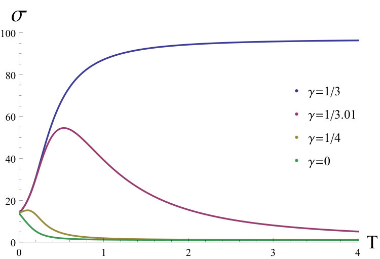 Figure 1
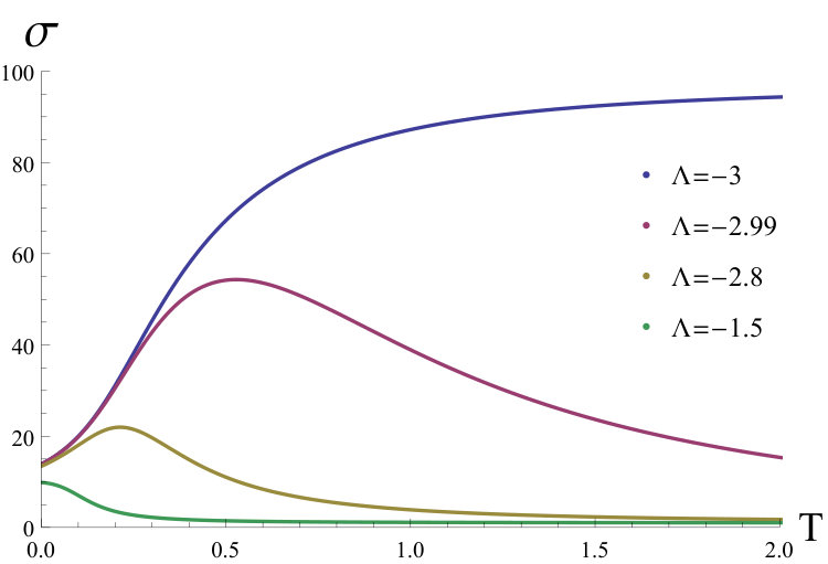 Figure 2
Peer Reviews
No public reviews on file for this paper yet. If you reviewed it on a platform where reviews are public (OpenReview, ICLR, NeurIPS, ICML), you can paste yours below so the community can read it here.
Videos
No videos yet. Explain this paper in a talk, walkthrough, or lecture? Add one.
MI-TH-1744
DC Conductivities with Momentum Dissipation in Horndeski Theories
Wei-Jian Jiang, Hai-Shan Liu, H. Lü and C.N. Pope
*Zhejiang Institute of Modern Physics, Zhejiang University, Hangzhou 310058, China *
*Institute for Advanced Physics & Mathematics,
Zhejiang University of Technology, Hangzhou 310023, China*
*George P. & Cynthia Woods Mitchell Institute for Fundamental Physics and Astronomy,
Texas A&M University, College Station, TX 77843, USA*
Department of Physics, Beijing Normal University, Beijing 100875, China
*DAMTP, Centre for Mathematical Sciences, Cambridge University,
Wilberforce Road, Cambridge CB3 OWA, UK*
ABSTRACT
In this paper, we consider two four-dimensional Horndeski-type gravity theories with scalar fields that give rise to solutions with momentum dissipation in the dual boundary theories. Firstly, we study Einstein-Maxwell theory with a Horndeski axion term and two additional free axions which are responsible for momentum dissipation. We construct static electrically charged AdS planar black hole solutions in this theory and calculate analytically the holographic DC conductivity of the dual field theory. We then generalize the results to include magnetic charge in the black hole solution. Secondly, we analyze Einstein-Maxwell theory with two Horndeski axions which are used for momentum dissipation. We obtain AdS planar black hole solutions in the theory and we calculate the holographic DC conductivity of the dual field theory. The theory has a critical point , beyond which the kinetic terms of the Horndeski axions become ghost-like. The conductivity as a function of temperature behaves qualitatively like that of a conductor below the critical point, becoming semiconductor-like at the critical point. Beyond the critical point, the ghost-like nature of the Horndeski fields is associated with the onset of unphysical singular or negative conductivities. Some further generalisations of the above theories are considered also.
Emails: [email protected] [email protected] [email protected]
Contents
1 Introduction
Gauge/Gravity duality has served as a powerful tool in understanding the phenomena of strongly coupled systems in condensed matter physics [1, 2, 3]. Especially, much attention has been paid to the holographic description of systems with momentum relaxation. Such systems with broken translational symmetry are needed in order to give a realistic description of materials in many condensed matter systems.
Since momentum is conserved in a system with translational symmetry, a constant electric field can generate a charge current without current dissipation in the presence of non-zero charge density. Thus, the conductivity of the system would become divergent at zero frequency. In more realistic condensed matter materials, the momentum is not conserved due to impurities or a lattice structure, thus leading to a finite DC conductivity.
In the context of holography, there are various ways to achieve momentum dissipation, such as periodic potentials, lattices and breaking diffeomorphism invariance [4, 5, 6, 7, 8, 9, 10, 11, 12, 13, 14, 15, 16, 17, 18]. Among these, the model in [12] is particular simple. It comprises an Einstein-Maxwell theory together with a set of minimally-coupled massless scalar fields that have linear dependence on the boundary coordinates. These axionic scalars preserve the homogeneity of the bulk stress tensor, since they have no mass terms or interactions that would break translational invariance.
In this paper, we shall generalise the models with momentum dissipation that were constructed in [12] by introducing non-minimal Horndeski type couplings of some of the scalar fields to gravity. The Horndeski theories were first constructed in the 1970s [19], and they have received much attention recently through their application to cosmology in Galileon theories (see, for example, [20]). A characteristic feature of Horndeski theories is that although terms in their Lagrangians involve more than two derivatives, the field equations and the energy-momentum tensor involve no higher than second derivatives of the fields. This is analogous to the situation in Lovelock gravities [21].
Specifically, we shall generalise the model in [12] in two parallel ways. Firstly, in section 2, we shall consider a Horndeski extension of an Einstein-Maxwell plus scalar theory in which two minimally-coupled axions that provide the momentum dissipation are supplemented by a third axion with a non-minimal Horndeski coupling. Although this axion has a significant effect in terms of modifying the geometrical structure of the black hole background, we find that the DC conductivity in the boundary theory is essentially unaltered, at least if one expresses the result as a function of the black hole horizon radius. In section 3, we shall consider instead an Einstein-Maxwell theory with Horndeski couplings to the two axions that provide the momentum dissipation. Here, we find that the effects of the non-minimal Horndeski couplings are much more substantial, and in fact as the strength of the non-minimal term is increased to a critical value, the qualitative behaviour of the conductivities as a function of temperature changes. Below the critical coupling the high-temperature behaviour is similar to that of a metal, whilst at the critical coupling the behaviour becomes more like that of a semiconductor. We summarize our results in section 4. In appendix, we extend the theories and solutions that we studied in the main text to arbitrary spacetime dimensions.
2 Momentum dissipation with Horndeski term
2.1 Electrical black hole
In this section, we consider AdS planar black holes of Horndeski theory in four dimensions. The solutions have been constructed in [22, 23], and the thermodynamics have been studied in [24, 25]. In these solutions, the Horndeski axion depends on the radial coordinate. In order to achieve momentum dissipation, we include two additional free axions as in [12]:
[TABLE]
where , , are coupling constants, is the Einstein tensor, and is the electromagnetic field strength. The equations of motion with respect to the metric , the Maxwell potential , the Horndeski scalar and the axions are given by
[TABLE]
One of the remarkable properties of a Horndeski theory is that each field has no higher than second-derivative terms in the equations of motion, even though the Lagrangian involves larger numbers of derivatives (up to four derivatives, in our case). Although terms quadratic in second-derivatives are present, linearised perturbations around a background will involve at most second-order linear differential equations, and thus can be ghost free.
We are interested in static planar black hole solutions in this paper. In this section, we shall take the Horndeski axion to depend only on the radial coordinate, whilst the two additional axions span the planar directions:
[TABLE]
where is a constant. The Maxwell equation can be used to express the electrostatic potential in terms of the metric functions, as
[TABLE]
where is an integration constant, parameterising the electric charge, and a prime denotes a derivative with respect to . The equation of motion for the Horndeski scalar can then be written as
[TABLE]
Following [22, 23], we focus on the special class of solutions obtained by taking
[TABLE]
With this, we can solve the Einstein equations and obtain the black hole solution
[TABLE]
where the parameters are such that
[TABLE]
The solution has non-trivial integration constants , and , together with a pure gauge parameter . The Hawking temperature can be calculated by standard methods, and is given by
[TABLE]
where is the radius of event horizon, which is the largest root of .
2.2 DC conductivity
There are many ways to compute the holographic conductivities. For the DC conductivity, a simple method makes us of the “membrane paradigm” [17, 26, 27, 28, 29, 30, 31]. The key point is to construct a radially conserved current, which allows one to read off the holographic boundary properties in terms of the black hole horizon data. Here, we shall follow the procedure described in [28].
We consider perturbations around the black hole solutions, of the form
[TABLE]
The equation of motion for the vector field implies that we can define a radially-conserved current
[TABLE]
Explicitly, this current is given by
[TABLE]
and it obeys .
The Einstein equations imply111Note that the perturbation is non-dynamical, and could in fact be removed by a coordinate transformation. We choose to keep it here in order to make the presentation parallel with the one we shall give below when a magnetic field is turned on, since in that case one cannot remove the analogous perturbations by means of a coordinate transformation.
[TABLE]
Regularity on the horizon requires that
[TABLE]
The last equation in (2.22) shows that near horizon,
[TABLE]
With these, we can evaluate the current on the horizon, finding
[TABLE]
and hence the conductivity is given by
[TABLE]
Interestingly, even though the theory we are considering here, and its black hole solutions, are much more complicated than the Einstein-Maxwell theory with linear axions that was studied in [12], the Horndeski scalar does not explicitly contribute to the conductivity when is expressed in terms of , and hence the result (2.26) is the same as in [12]. Of course, the Horndeski term modifies the relation between the temperature and , and so in the relation the Horndeski term has non-trivial effects. However at large (corresponding to large , with ), the dependence approaches that obtained in [12].
2.3 Dyonic black hole
We can obtain a more general class of dyonic black hole solutions, by extending the ansatz for the vector potential in (2.8) to include a magnetic term:
[TABLE]
We find the dyonic black hole solution is given by
[TABLE]
It is interesting to note that this dyonic solution is rather simply related to the previous purely electric solution by means of a replacement in which the quadratic powers of in (2.15) are sent to , while the linear powers of are left unchanged, in the sense that one makes the formal replacements
[TABLE]
The Hawking temperature for the dyonic black hole is given by
[TABLE]
We are now in a position to calculate the DC conductivity in the dyonic black hole background. In this case, we turn on perturbations in both the spatial boundary directions ,
[TABLE]
Following similar methods to those we used in the previous subsection, we construct a radially-conserved 2-component current
[TABLE]
The regularity conditions on the horizon are
[TABLE]
The currents can be evaluated on the horizon, and we define the conductivity matrix by
[TABLE]
Explicitly, the conductivity matrix elements are given by
[TABLE]
The Hall angle is defined (for small angles) by
[TABLE]
As in the purely electrically-charged black holes, the inclusion of the Horndeski scalar does not modify these transport quantities when they are expressed in terms of the variable. In particular the Hall angle goes to zero at high temperature, as .
3 Momentum dissipation using Horndeski axions
3.1 Dyonic black hole
In this section, we consider a system in which the axionic scalars that provide the momentum dissipation are themselves taken to have Horndeski couplings rather than minimal couplings to gravity. The Lagrangian describing the theory is given by
[TABLE]
We shall assume that is positive, and so for we recover the Einstein-Maxwell theory with two free axions, proposed in [12]. The equations of motion are
[TABLE]
It is clear that these equations admit a pure AdS vacuum solution where and the electromagnetic and scalar fields vanish. In this vacuum, the effective kinetic term for the Horndeski axions becomes
[TABLE]
This will be of the standard sign, signifying ghost-freedom, if . In this paper we shall consider only solutions for which is negative. Stability requires that should be non-negative, but novel features can arise at the critical point where vanishes. (An analogous situation can also arise in Einstein-Gauss-Bonnet theories, see, e.g., [32].) Thus can lies in the range
[TABLE]
Typically, the cosmological constant is viewed as a fixed parameter that is part of the specification of a theory, but it can alternatively arise as an integration constant for an -form field strength in dimensions. Thus here we may replace the cosmological constant term in (3.1) by a term
[TABLE]
The equation of motion for can be solved by taking , where is an arbitrary non-positive constant that acquires an interpretation as the cosmological constant. In this new theory, one may treat the “cosmological constant” as a thermodynamic variable, which has an interpretation as a pressure (see, for example, [33, 34]). Changing the cosmological constant, i.e. the pressure, can lead to a phase transition from a stable to an unstable regime as the sign of turns negative. The critical point where vanishes gives, as we shall see, some interesting features in the boundary theory.
We now construct dyonic AdS planar black holes where the two Horndeski axions are linear functions of the spatial boundary coordinates , i.e.,
[TABLE]
The equations of motion for the axions are trivially satisfied. The Maxwell equation implies that
[TABLE]
where is an integration constant. With this, the Einstein equations give
[TABLE]
These equations can be easily solved, leading to the black hole solutions
[TABLE]
where erfi is the imaginary error function, defined by erfi. The asymptotic forms of the metric functions near infinity are given by
[TABLE]
which shows that the solution is asymptotic to dS or AdS for or respectively. Since we are interested in the transport properties of the dual boundary theory, we shall focus on the AdS case, and so we shall assume in the rest of this section. The Hawking temperature is given by
[TABLE]
Although the linearised equations of motion for the Horndeski terms are of two derivatives, it is still necessary to check the sign of the kinetic terms for possible ghost-like behaviour. The kinetic terms for the perturbative axions are given by
[TABLE]
In order to avoid ghosts, the component of , which is given by
[TABLE]
should be non-negative, both on and outside the horizon. The asymptotic form of near infinity is given by
[TABLE]
The positivity of therefore implies, as a necessary condition, that (assuming, as we are, that ). In the case of equality, , the leading term of vanishes and the asymptotic form of becomes simpler, with
[TABLE]
which is still greater than zero. It can then be checked from (3.22) that is indeed always positive in the region from the horizon to infinity when and are both positive.
3.2 DC conductivity and Hall angle
Now, we turn to the calculation of the DC conductivity of this system. We follow a similar procedure to the one described in the previous section. Here we shall omit the details of the calculation, and just present the final results. We begin with the simpler case where , for which we find the conductivity is given by
[TABLE]
When , this result reduces to (2.26). This demonstrates that the couplings of the axions for dissipative momenta plays a crucial role in shaping the conductivity. Although contains the same “charge-conjugation symmetric” term , as one would expect, it has a very different “dissipative” term associated with that has a richer structure. At large , however, it has the same qualitative behaviour as that of the Einstein-Maxwell case in the high-temperature limit for generic parameters
[TABLE]
On the other hand, at the critical point , the temperature dependence is characteristically different. The denominator of the dissipative term in (3.25) has three contributions, with the leading-order power of being proportional to . When is positive, the conductivity rises from a positive in initial value at zero temperature, rises to a peak, and then decreases to a constant value at high temperature. 222This phenomenon was observed in [18], where massive gravity was used to achieve momentum dissipation. Especially, when , the conductivity decreases monotonically from its initial value as the temperature increases, behaving much like a normal conductor. If on the other hand , the conductivity monotonically increases with temperature, approaching a constant in the high-temperature limit. This behaviour is closer to that of a semiconductor. We illustrate the various behaviours in Fig.1, where the parameters are fixed such that and . In the left-hand diagram we fix also and display the plots of versus for four representative values of . The top curve corresponds to the critical case , while the lower curves correspond cases with . In the right-hand diagram we instead fix and display plots for various values of , again with the critical case being the curve at the top, with the lower curves having . The critical case can be thought of as representing a phase transition where the high-temperature behaviour of the material changes from that of a metal ( falls to a small constant as increases) to a semiconductor ( rises to a limiting value as increases) in the critical case. From the bulk point of view, the transition can be viewed as being induced when the pressure () becomes sufficiently large.
It is interesting to note that in the left-hand diagram in Fig. 1, all the conductivity curves originate from the same value when . The reason for this can be seen from the expressions for the temperature and the conductivity, namely
[TABLE]
The temperature becomes zero when the factor in parentheses in (3.27) vanishes, and then (3.28) implies that the corresponding zero-temperature conductivity is given by
[TABLE]
with being given by
[TABLE]
Thus at fixed , with , , and also fixed as in left-hand diagram, the zero-temperature conductivity is independent of . By contrast, if is fixed instead of , as in the right-hand diagram, the zero-temperature conductivity does depend on .
We have not included plots for values of the parameters for which is negative. Here, the dissipative part of the conductivity can be negative, and for a range of temperatures the full expression for the conductivity can be negative or divergent. This suggests an unphysical instability, and is in fact consistent with our previous observation that the Horndeski axions acquire ghost-like kinetic terms when is negative.
The case when is considerably more complicated, and we shall not present the general expression for the conductivity matrix here. However, in the high temperature limit we find that it takes the form for
[TABLE]
and the Hall angle is given by
[TABLE]
At the critical point , the conductivity and Hall angle at high temperature become
[TABLE]
In particular, the Hall angle approaches a constant at large . At , on the other hand, which occurs when the factor in parentheses in the numerator in (3.20) vanishes, the conductivity and Hall angle become
[TABLE]
where
[TABLE]
It is of interesting to note that at , both ’s and are independent of . This implies that in the zero temperature limit the DC conductivities and Hall angle are the same as those in the Einstein-Maxwell case (2.41,2.42), if the results are expressed in terms of the horizon radius and we set .
4 Conclusions
In this paper, we studied two four-dimensional gravity theories involving scalar fields with non-minimal Horndeski-type couplings to gravity. We first considered Einstein-Maxwell gravity with one non-minimally coupled Horndeski axion and two minimally coupled axions. The two minimally coupled axions have linear dependence on the spatial boundary coordinates, and they generate momentum dissipation in the standard way. We constructed a charged AdS planar black hole in the theory, and calculated the holographic DC conductivity in the dual field theory. Interestingly, although the Horndeski scalar in these solutions plays a role in determining the geometry of the black hole background, it does not contribute directly to the conductivity. To be precise, if written in terms of the horizon radius the conductivity is the same as that in Maxwell-Einstein gravity.
In the second model, we used two Horndeski axions, non-minimally coupled to Einstein-Maxwell gravity, to drive the momentum dissipation. We obtained a static AdS black hole solution in the theory. We analyzed the kinetic terms of the axion perturbations, and showed that the theory has a critical point at . When , the kinetic terms of the axion perturbations become negative, implying that the excitations become ghost-like. We then obtained the conductivity in the dual boundary theory, and found that the conductivity has two terms, a “charge-conjugation symmetric” term and “dissipative” term as usual. However, the dissipative term has richer features than in a standard minimally-coupled theory. At the critical point , the conductivity increases monotonically as a function of temperature, which is typical of the behaviour in a semiconductor. When , on the other hand, the conductivity rises to a maximum then falls, finally approaching a constant. In the special case , corresponding to turning off the Horndeski modification of the usual minimal coupling of the axions, the conductivity decreases monotonically with temperature, and the behavior is more like a normal conductor. We chose a set of parameters in the paper and plotted the conductivity versus temperature curves for various values of , in Fig. 1. We showed that from the critical point to the special case , the behavior of the conductivity as a function of temperature changes from that reminiscent of a semiconductor to that of a normal conductor.
Momentum dissipation is the key for obtaining finite holographic DC conductivity. While free axions provide one of the simplest models for such a mechanism, the resulting DC conductivity generally tends to have a fairly simple structure whose qualitative features are independent of the parameters. Our work demonstrated that using non-minimally coupled axions in the momentum-dissipation mechanism can lead to a much richer pattern of holographic DC conductivities.
Acknowledgements
We are grateful to Sera Cremonini for discussions. H-S.L. is supported in part by NSFC grants No. 11305140, 11375153, 11475148, 11675144 and CSC scholarship No. 201408330017. The work of H.L. is supported in part by NSFC grants No. 11475024, No. 11175269 and No. 11235003. C.N.P. is supported in part by DOE grant DE-FG02-13ER42020.
Appendix A Higher dimensional case
In this section, we generalise the theory in section 2 to include -form fields in arbitrary dimension,
[TABLE]
where , and are coupling constants, is the Einstein tensor, is the electromagnetic field strength and is one of the form fields which span all spacial dimension with . The equations of motion are given by
[TABLE]
We consider static planar black hole ansatz
[TABLE]
where is a constant. The Maxwell’s equation can be used to express the electrical potential in terms of metric functions
[TABLE]
where is an integration constant. And the equation of motion for scalar can be written as
[TABLE]
We focus on a special class of solution, as what we did in section 2, by letting
[TABLE]
Under these setup, we can obtain the black hole solution
[TABLE]
with parameters under constraint
[TABLE]
Appendix B Einstein-Maxwell-Dilaton theory with Horndeski axions
In section 3, we studied the theory of Einstein-Maxwell gravity with two non-minimally coupled Horndeski axions. Here, we give a generalisation in which we include also a dilatonic scalar field with an exponential coupling to the Maxwell field, and exponential potential terms. The Lagrangian is given by
[TABLE]
where and are constants. The second potential term, with coefficient , is required for the case where a magnetic field is included. The equations of motion are given by
[TABLE]
We consider the static planar black hole in four dimensions
[TABLE]
where and are constants. The Maxwell equation implies
[TABLE]
We find that there are two inequivalent classes of solutions, where the parameters are given by
[TABLE]
In both classes we have
[TABLE]
For class 1 we find
[TABLE]
with parameters
[TABLE]
Ei is the exponential integral, defined by
[TABLE]
The Hawking temperature for the class 1 solutions is given by
[TABLE]
The positivity of temperature require . In the large limit, the temperature approaches
[TABLE]
For the class 2 solutions we find
[TABLE]
with parameters
[TABLE]
The Hawking temperature for the class 2 solutions is given by
[TABLE]
It can be seen from the series expansion for the exponential integral function given in (B.13) that in the case of the class 2 solutions, the non-integer powers of that arise, for generic values of , in the large- expansion of the metric function can be removed altogether if the constant is chosen to be given by
[TABLE]
The reference list from the paper itself. Each links out to its DOI / PubMed record.
- 1[1] S.A. Hartnoll, Lectures on holographic methods for condensed matter physics , Class. Quant. Grav. 26 , 224002 (2009), ar Xiv:0903.3246 [hep-th].
- 2[2] S. Sachdev, What can gauge-gravity duality teach us about condensed matter physics? , Ann. Rev. Condensed Matter Phys. 3 , 9 (2012), ar Xiv:1108.1197 [cond-mat.str-el].
- 3[3] J. Mc Greevy, TASI lectures on quantum matter (with a view toward holographic duality) , ar Xiv:1606.08953 [hep-th].
- 4[4] G.T. Horowitz, J.E. Santos and D. Tong, Optical Conductivity with Holographic Lattices , JHEP 1207 , 168 (2012), ar Xiv:1204.0519 [hep-th].
- 5[5] G.T. Horowitz, J.E. Santos and D. Tong, Further Evidence for Lattice-Induced Scaling , JHEP 1211 , 102 (2012) ar Xiv:1209.1098 [hep-th].
- 6[6] G.T. Horowitz and J.E. Santos, General Relativity and the Cuprates , JHEP 1306 , 087 (2013) ,ar Xiv:1302.6586 [hep-th].
- 7[7] P. Chesler, A. Lucas and S. Sachdev, Conformal field theories in a periodic potential: results from holography and field theory , Phys. Rev. D 89 , no. 2, 026005 (2014), ar Xiv:1308.0329 [hep-th].
- 8[8] Y. Ling, C. Niu, J.P. Wu and Z.Y. Xian, Holographic Lattice in Einstein-Maxwell-Dilaton Gravity , JHEP 1311 , 006 (2013), ar Xiv:1309.4580 [hep-th].