Updated Global 3+1 Analysis of Short-BaseLine Neutrino Oscillations
S. Gariazzo, C. Giunti, M. Laveder, Y.F. Li

TL;DR
This paper updates the global analysis of short-baseline neutrino oscillation data within a 3+1 framework, considering recent experimental results and constraints, and identifies potential parameter regions for active-sterile neutrino mixing.
Contribution
It provides an updated global fit of short-baseline neutrino oscillation data, incorporating recent experimental constraints and analyzing the viability of sterile neutrino explanations for anomalies.
Findings
Identifies three narrow allowed regions for $ u_4$ mass-squared difference around 1.3-2.4 eV$^2$.
Reveals tension between appearance and disappearance data, alleviated by excluding MiniBooNE low-energy anomaly.
Suggests ongoing experiments will clarify the sterile neutrino hypothesis.
Abstract
We present the results of an updated fit of short-baseline neutrino oscillation data in the framework of 3+1 active-sterile neutrino mixing. We first consider and disappearance in the light of the Gallium and reactor anomalies. We discuss the implications of the recent measurement of the reactor spectrum in the NEOS experiment, which shifts the allowed regions of the parameter space towards smaller values of . The beta-decay constraints allow us to limit the oscillation length between about 2 cm and 7 m at for neutrinos with an energy of 1 MeV. We then consider the global fit of the data in the light of the LSND anomaly, taking into account the constraints from and disappearance experiments, including the recent data of the MINOS and IceCube experiments. The combination of the NEOS constraints on and…
Click any figure to enlarge with its caption.
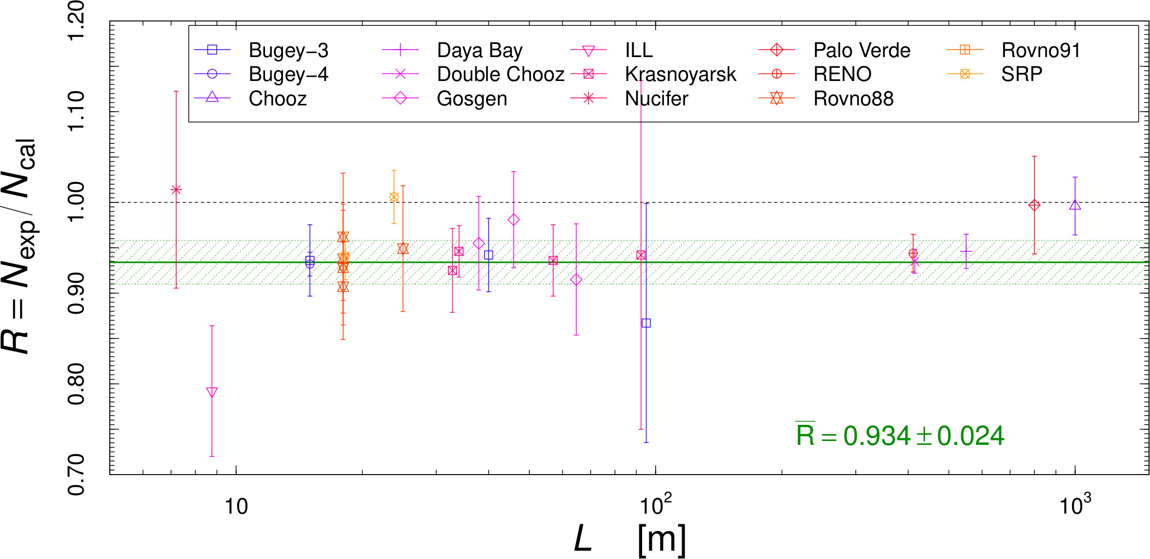 Figure 1
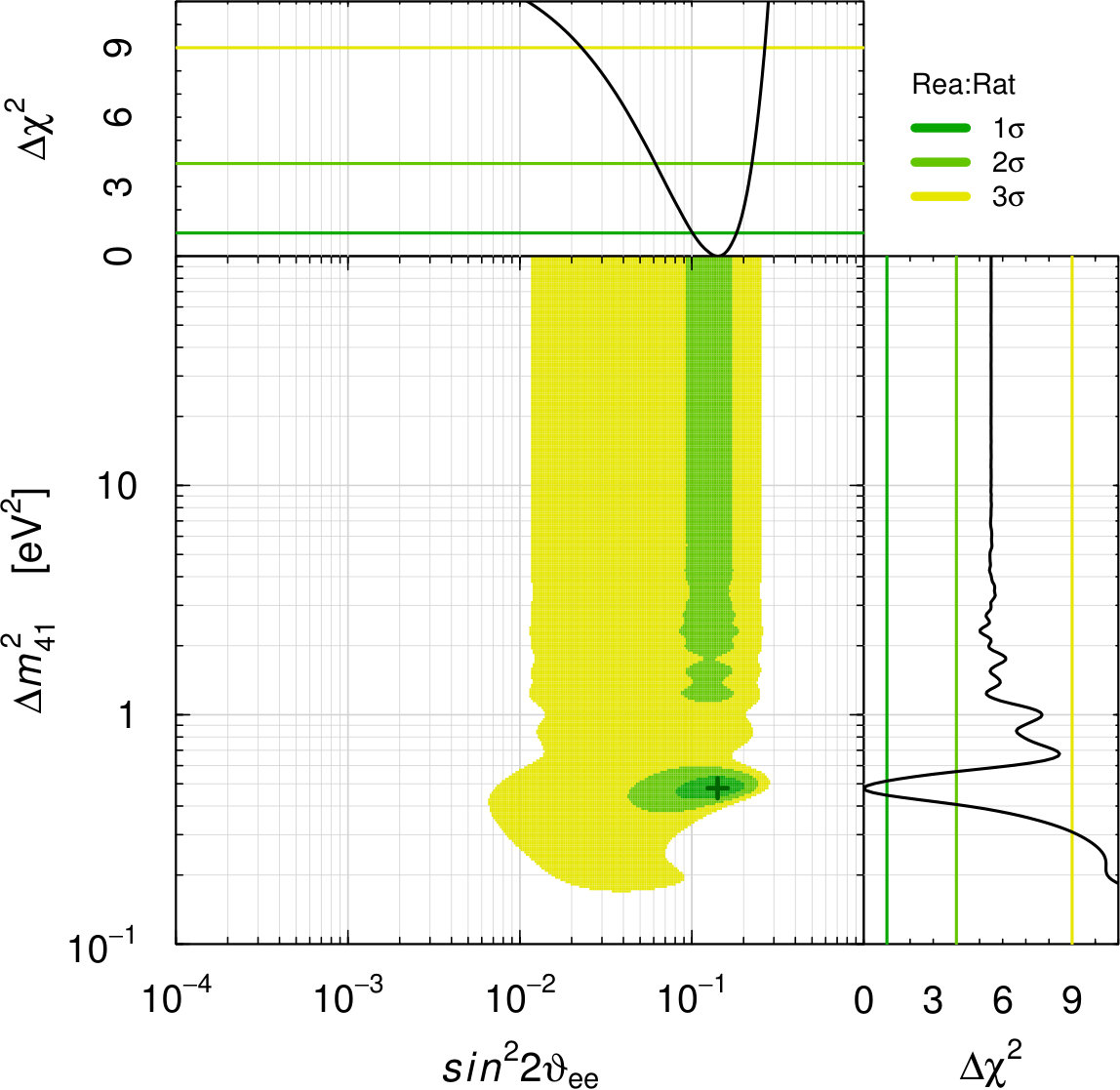 Figure 2
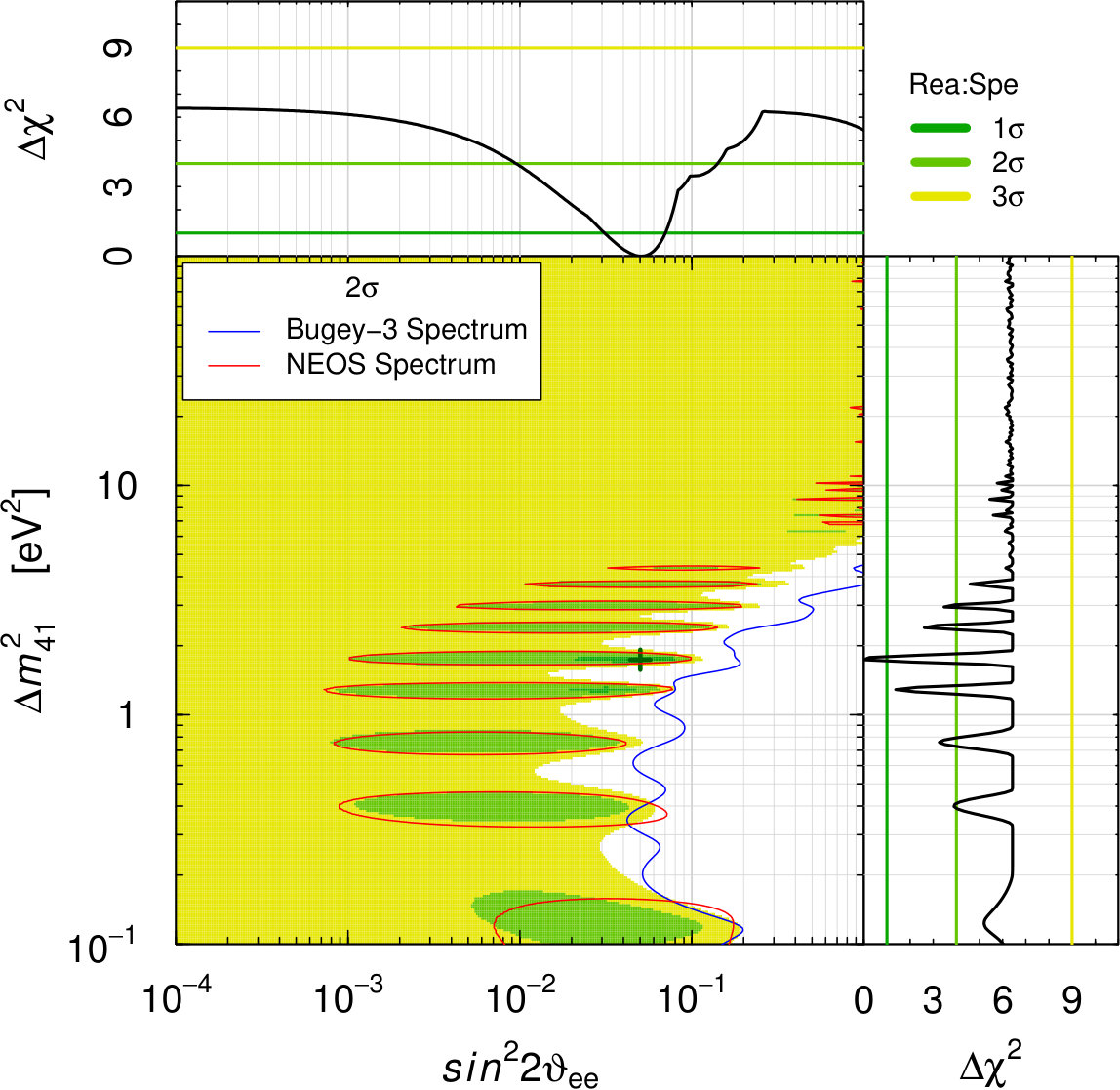 Figure 2
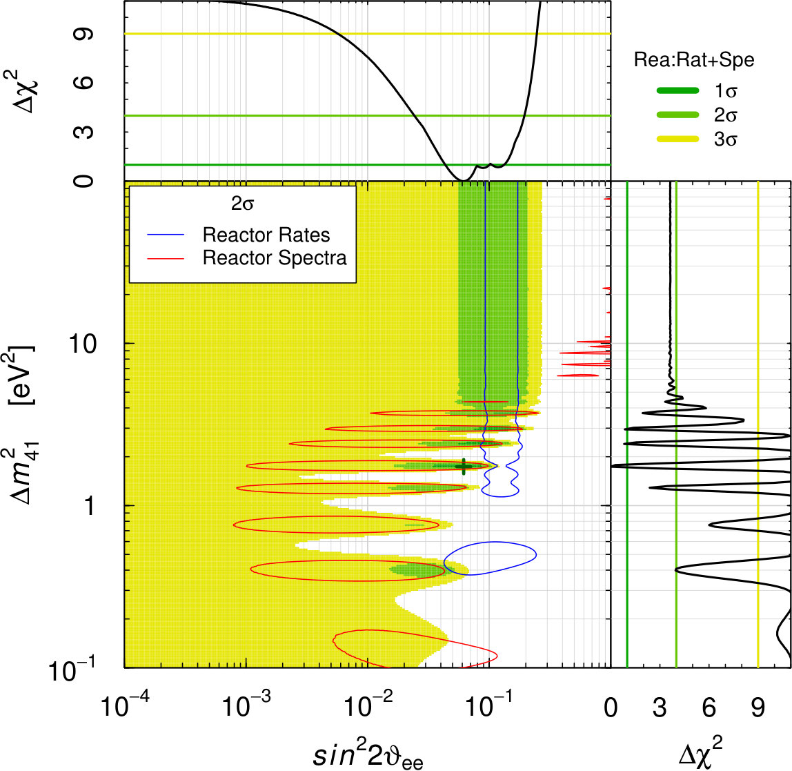 Figure 3
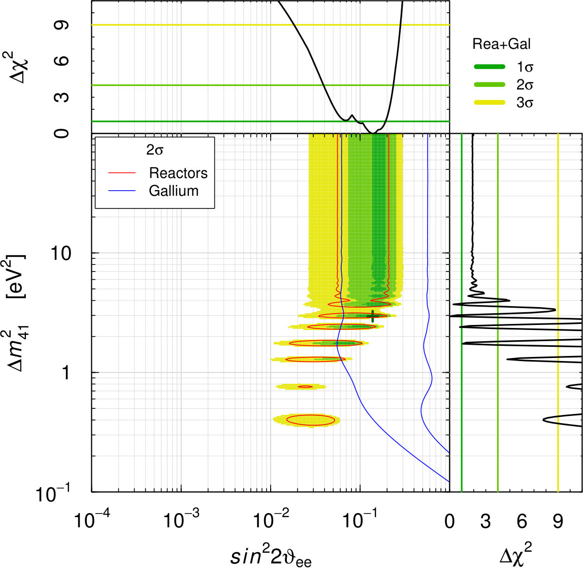 Figure 3
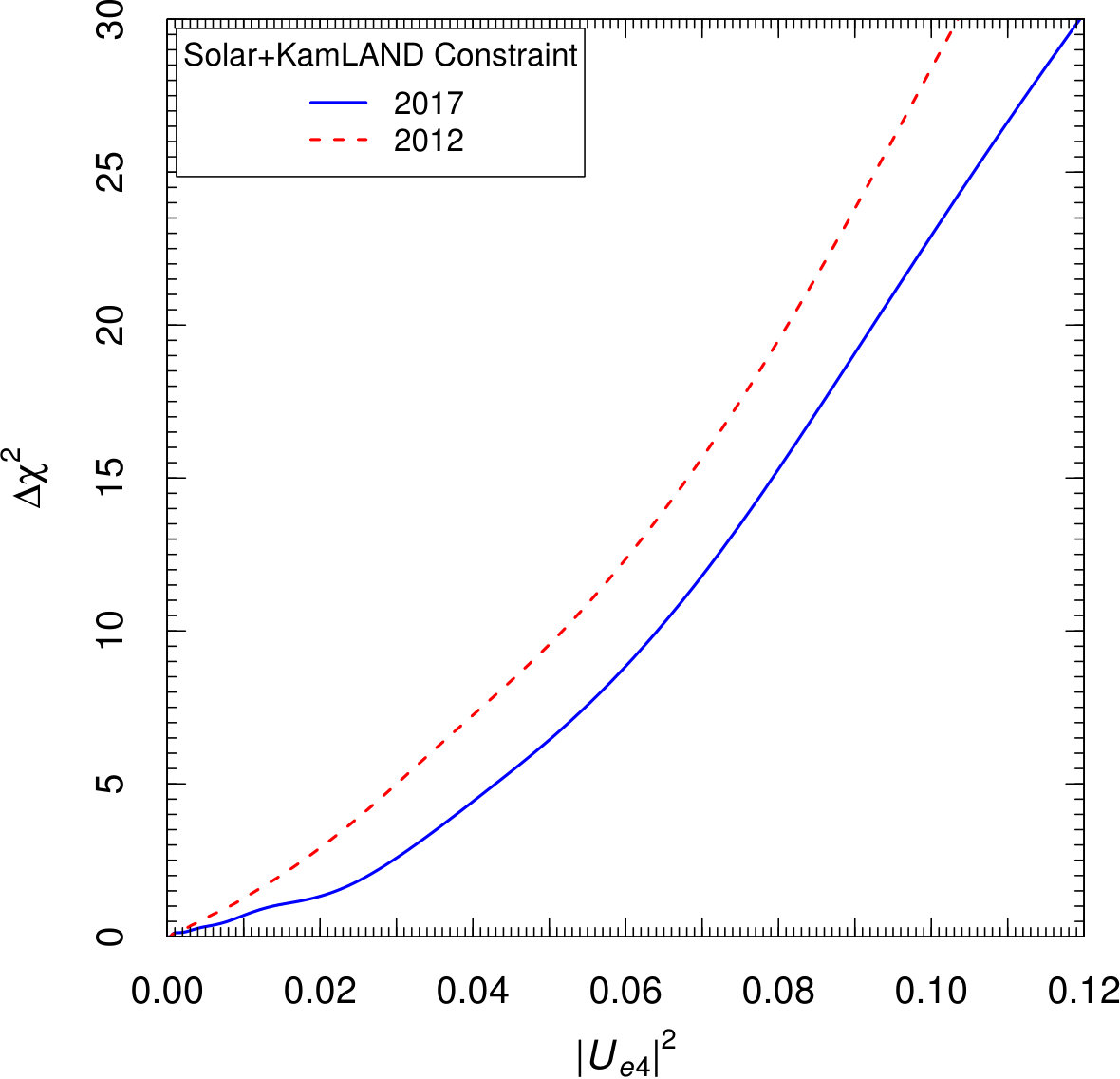 Figure 4
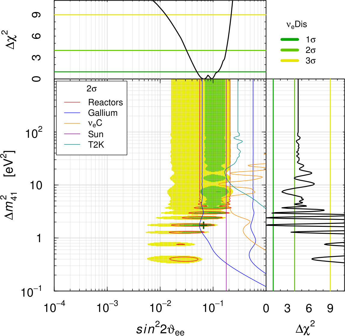 Figure 5
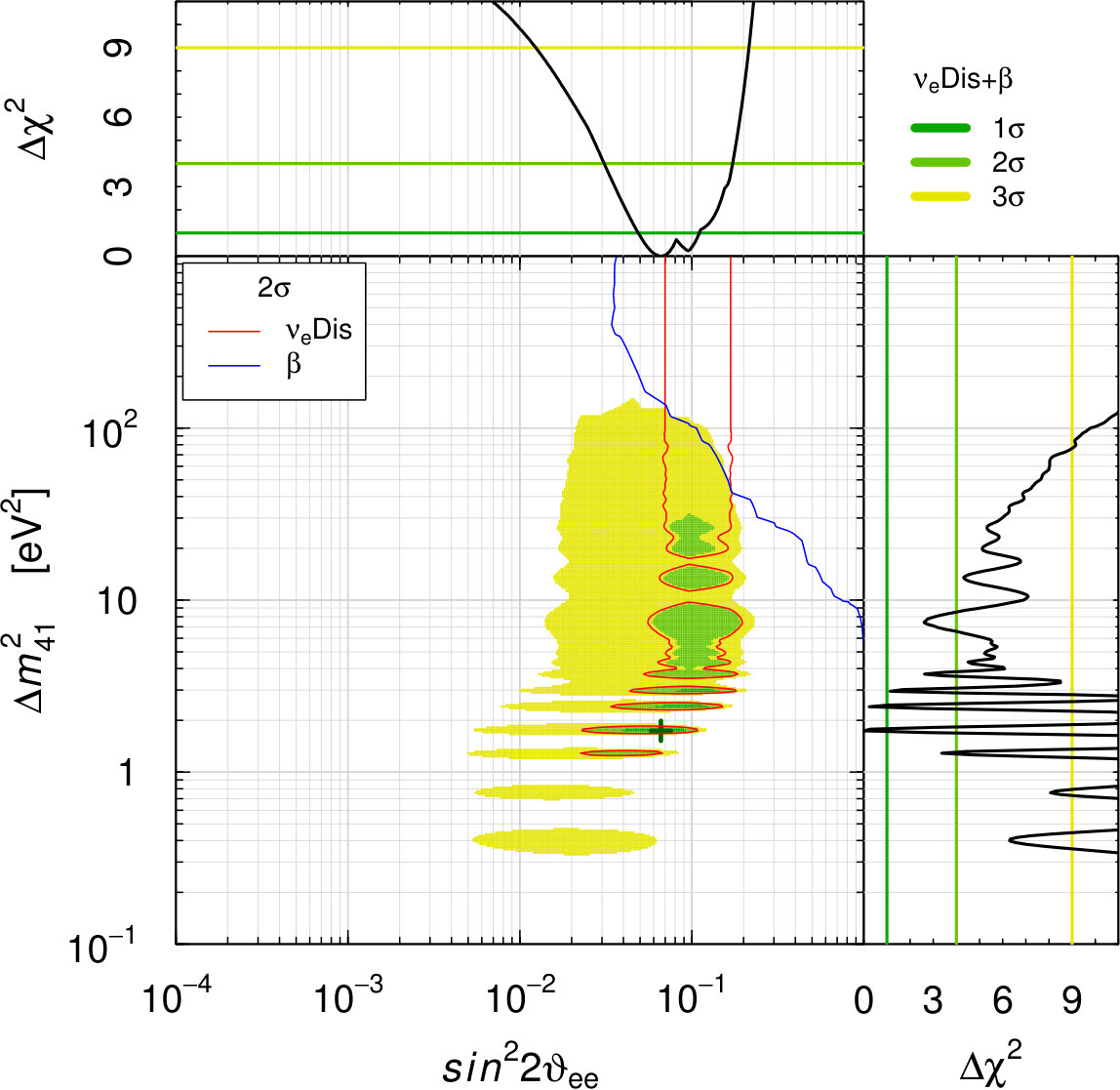 Figure 5
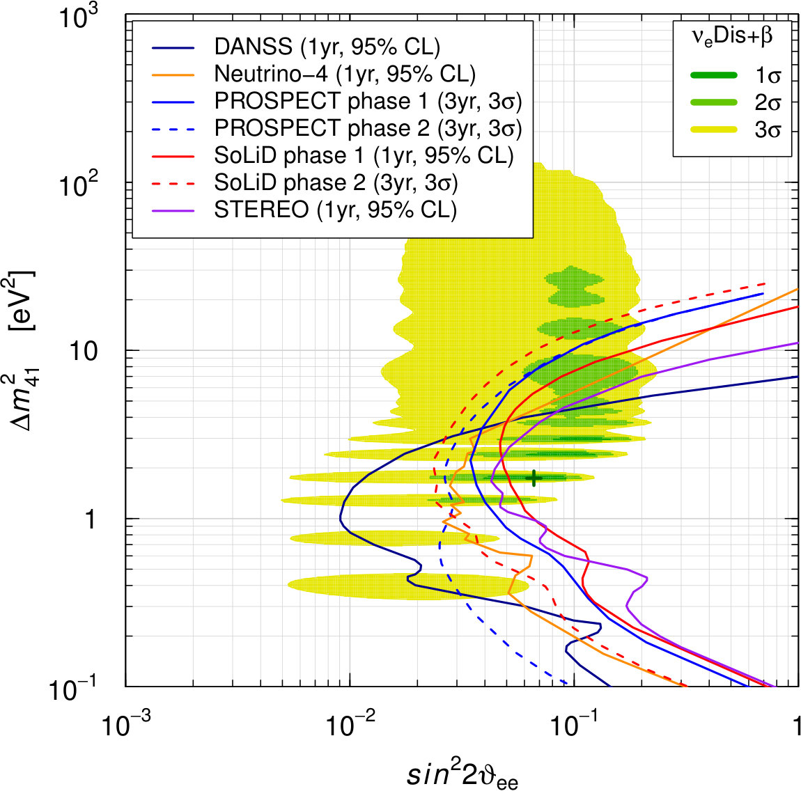 Figure 6
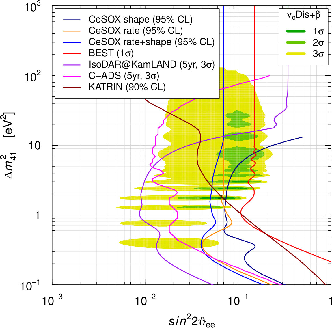 Figure 6
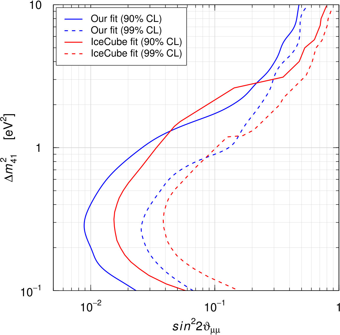 Figure 7
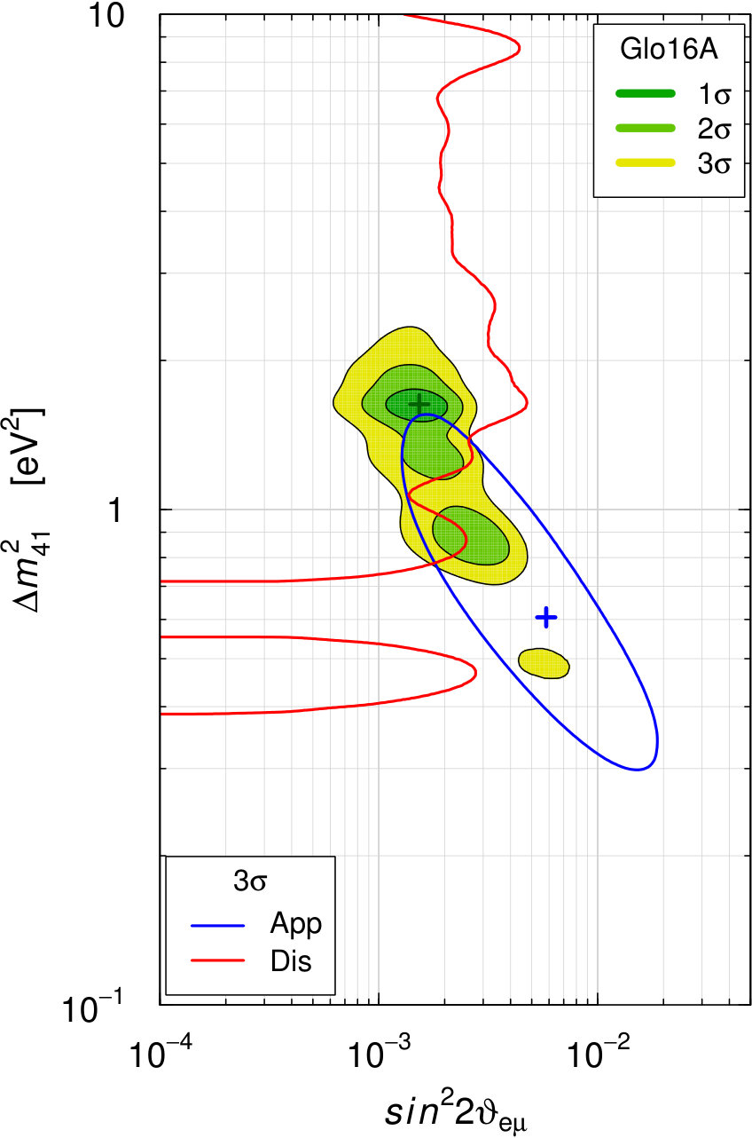 Figure 8
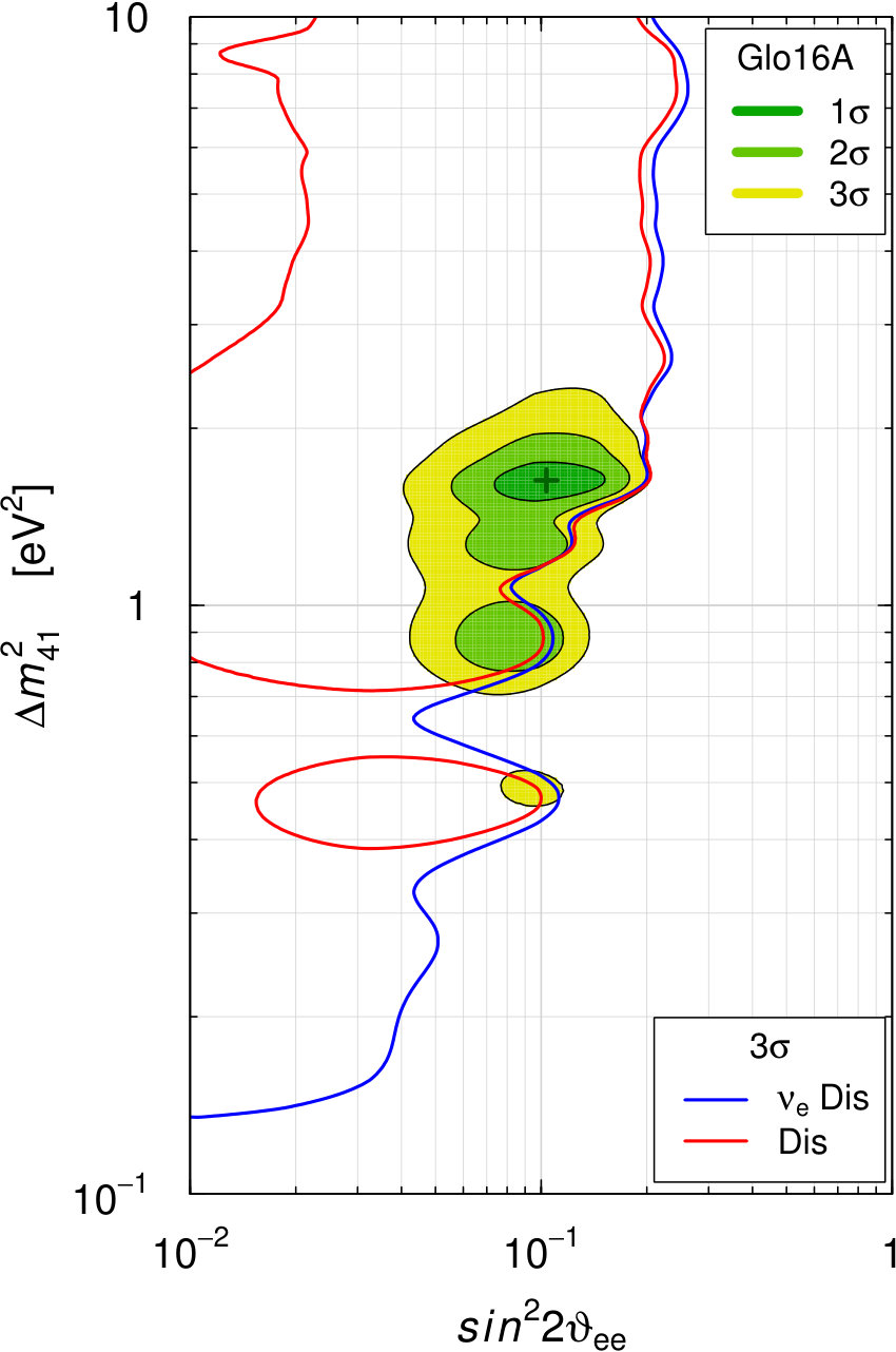 Figure 8
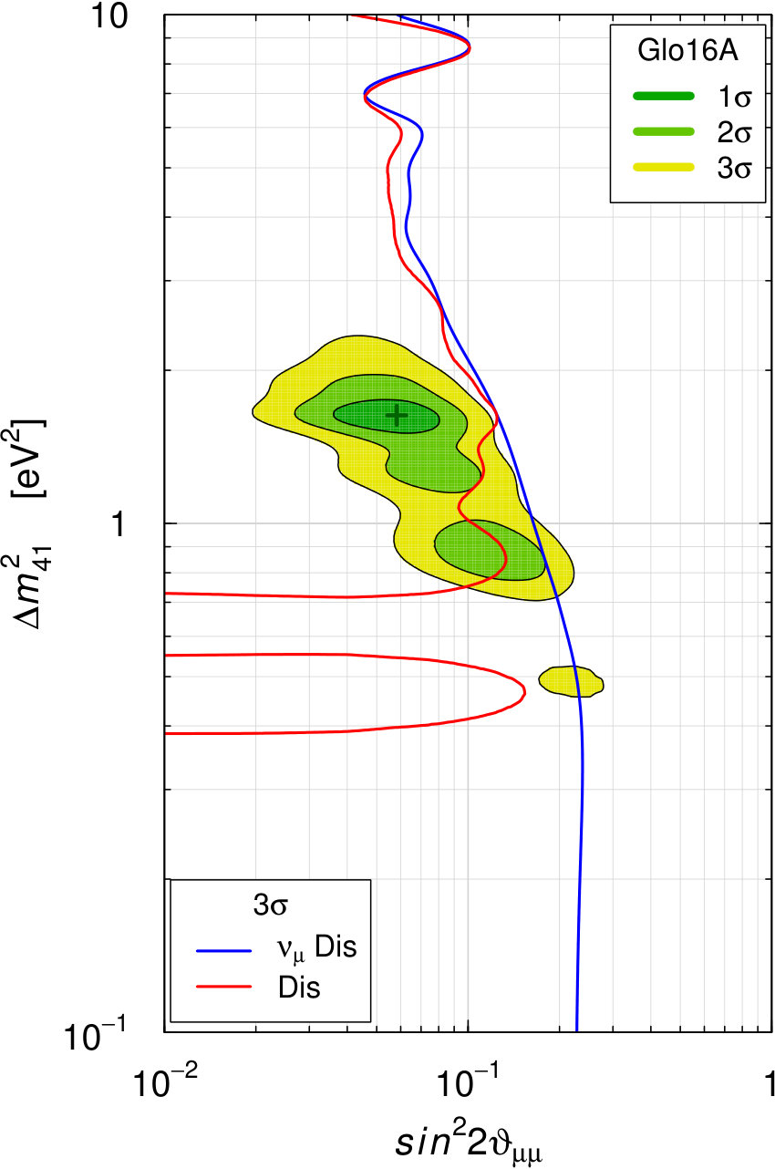 Figure 8
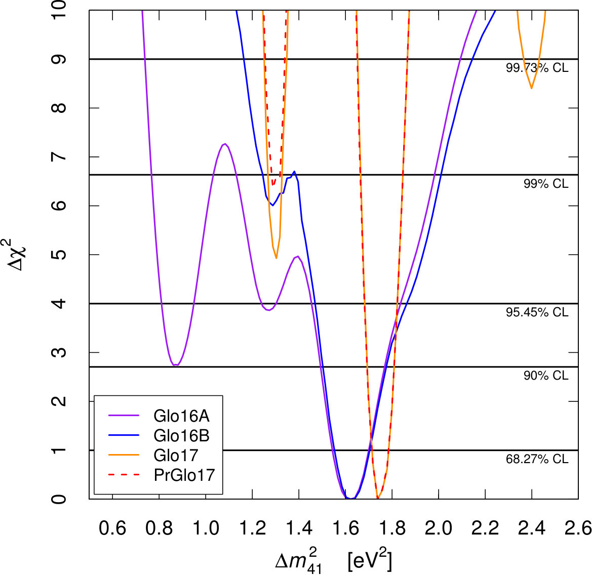 Figure 9
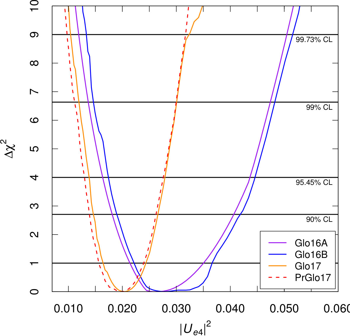 Figure 9
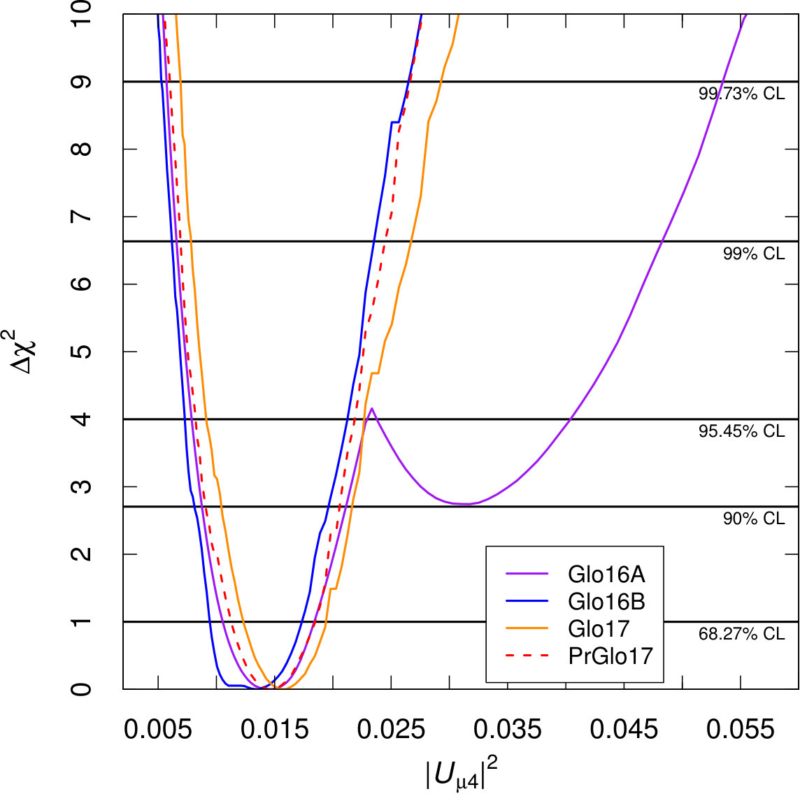 Figure 9
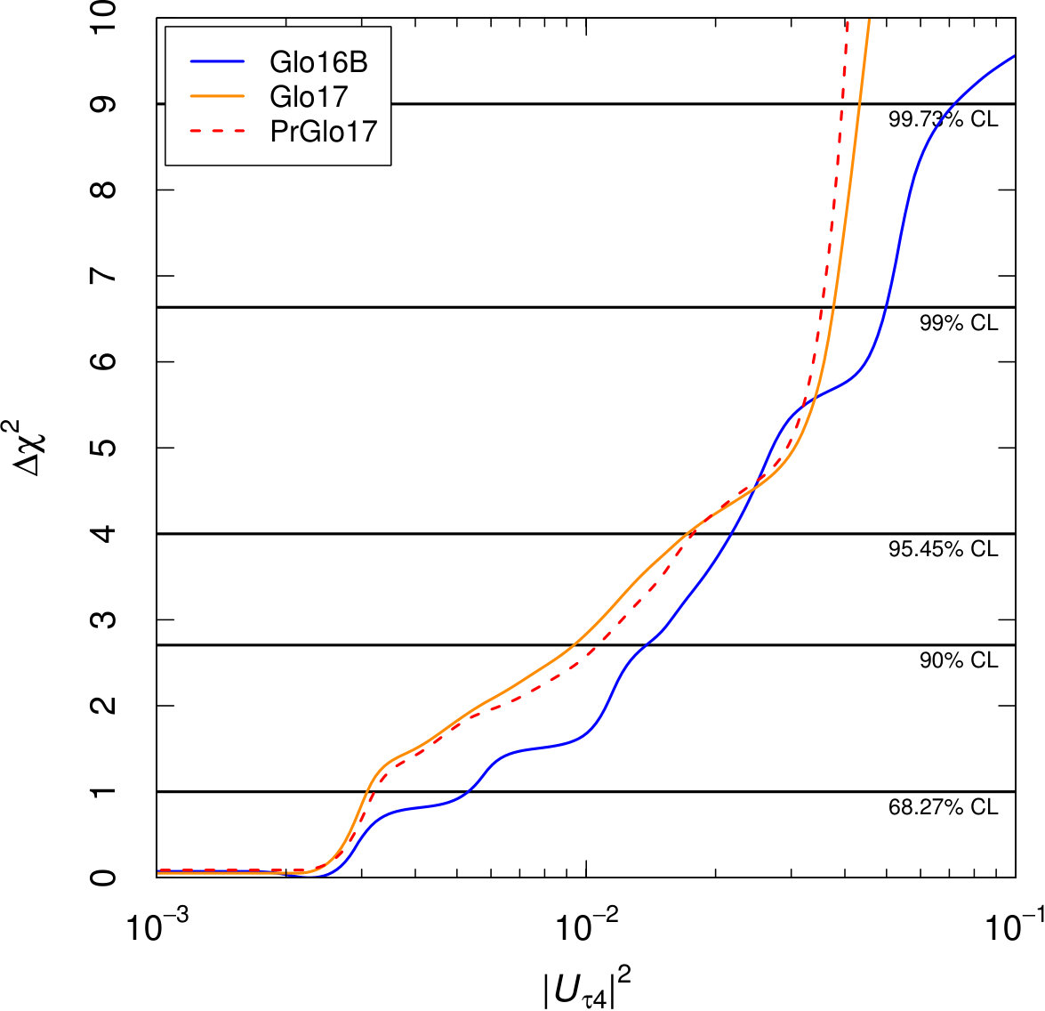 Figure 9
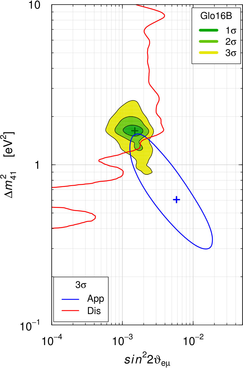 Figure 10
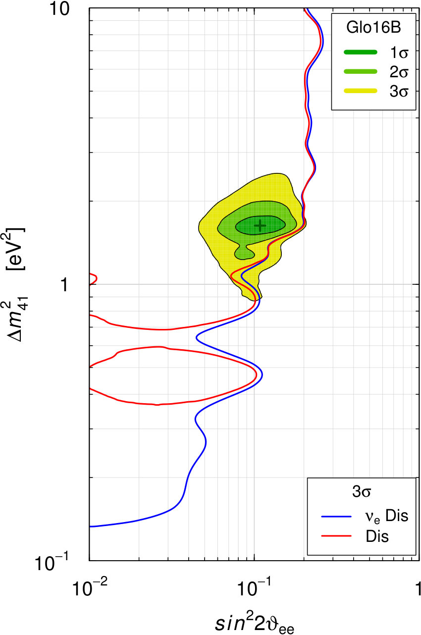 Figure 10
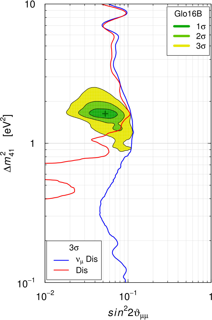 Figure 10
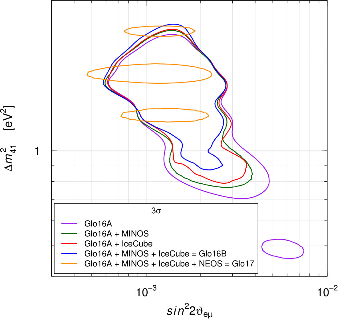 Figure 11
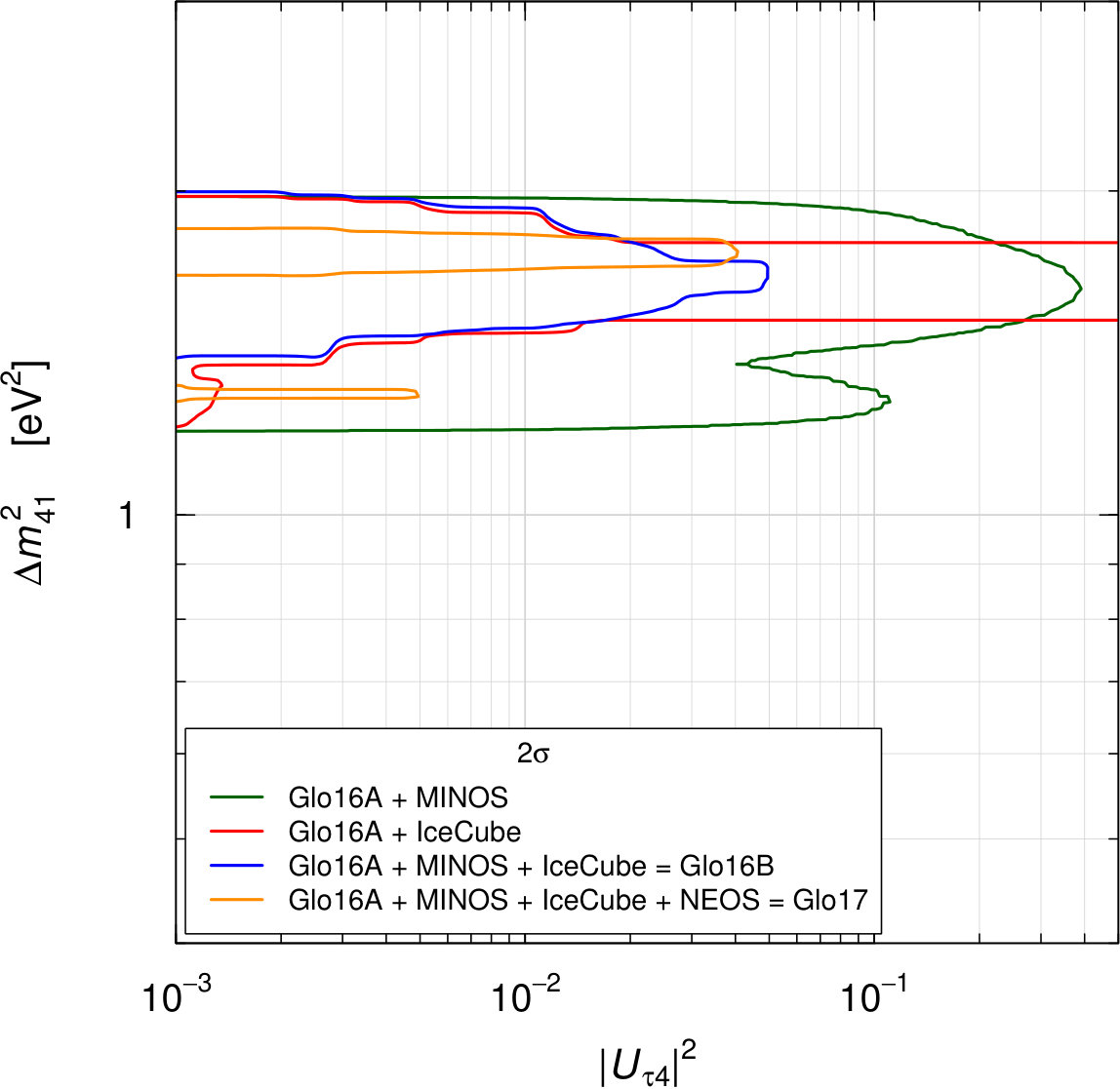 Figure 11
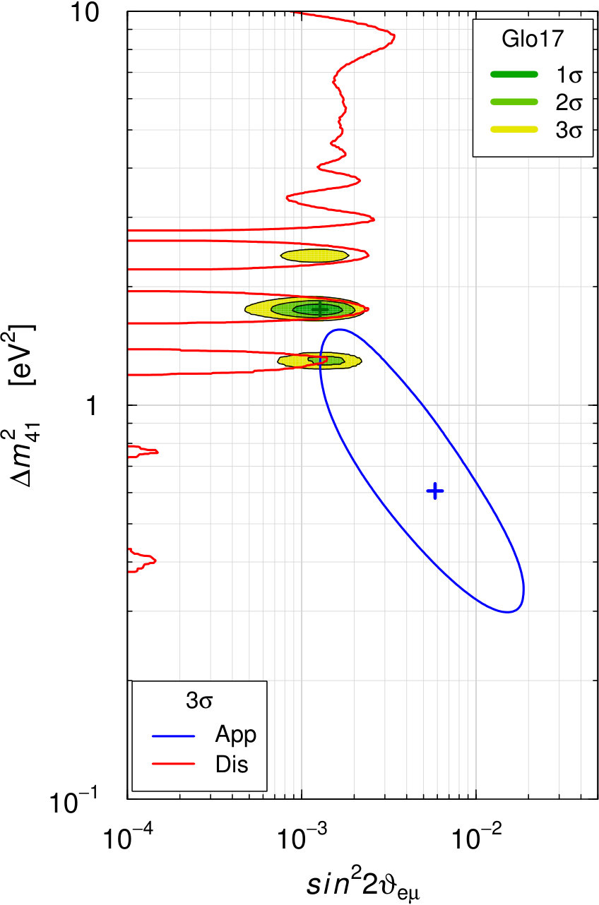 Figure 12
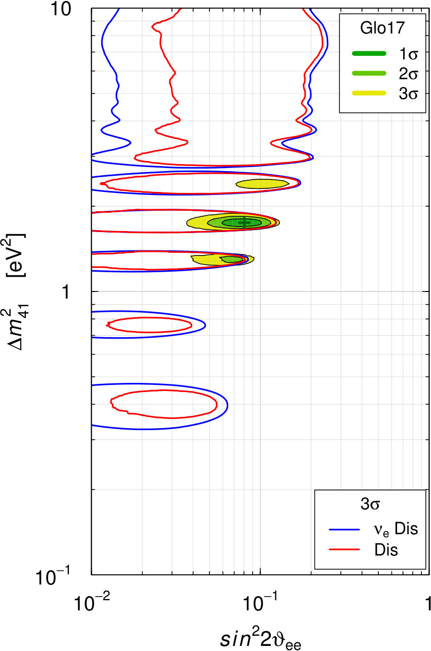 Figure 12
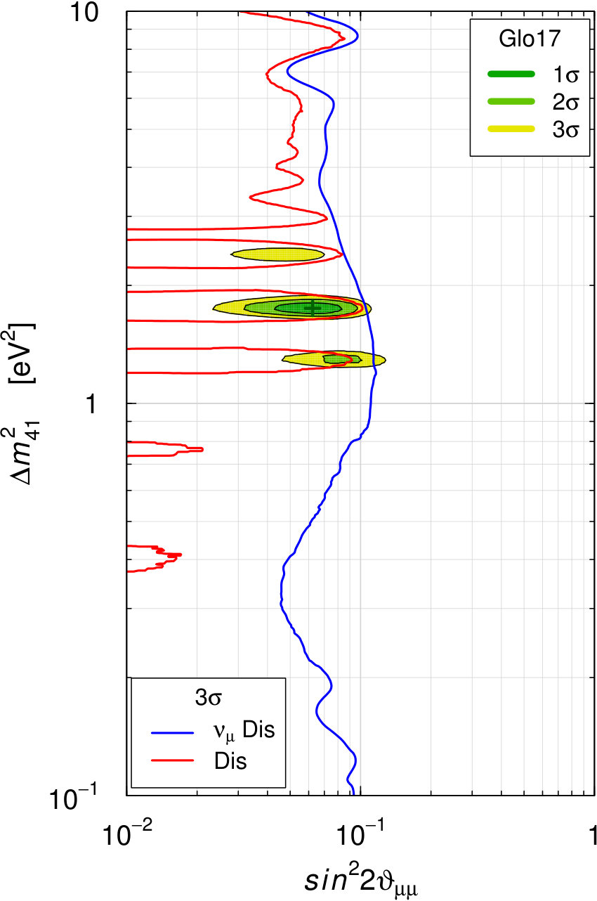 Figure 12
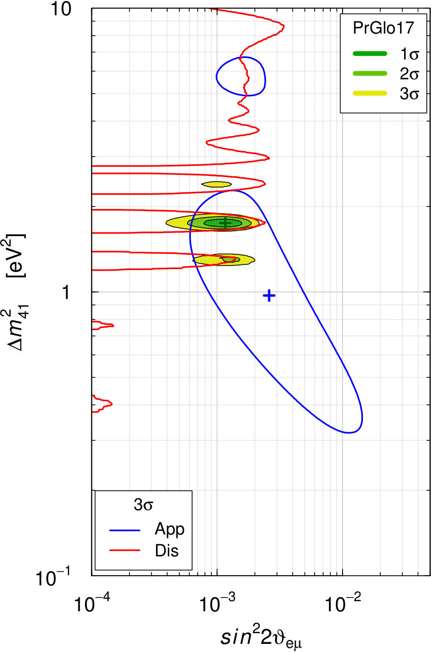 Figure 13
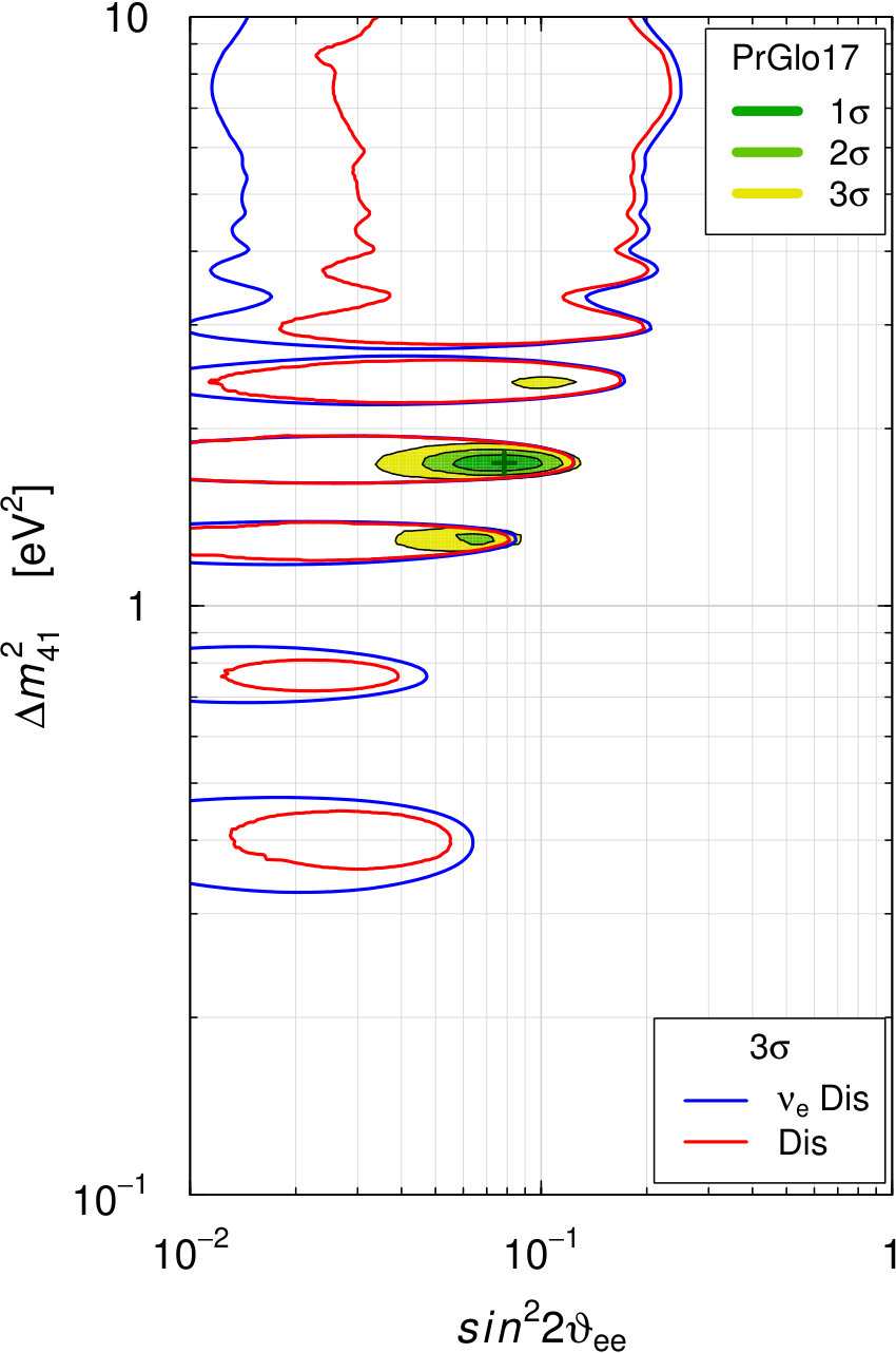 Figure 13
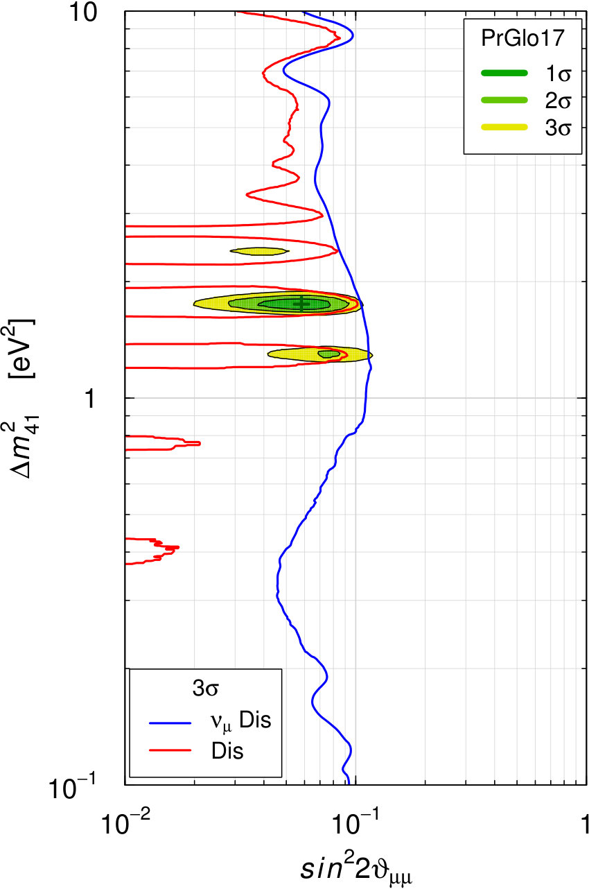 Figure 13
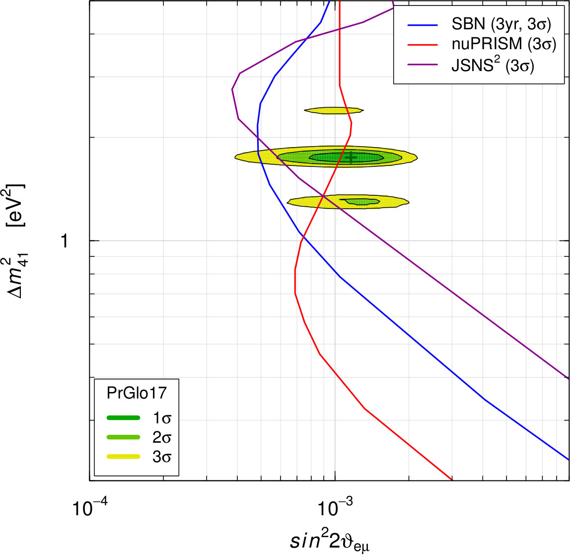 Figure 14
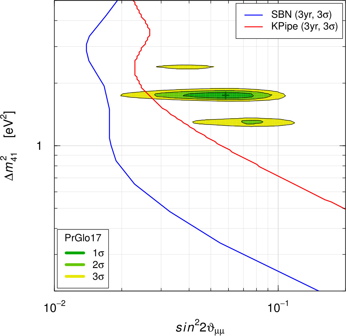 Figure 14
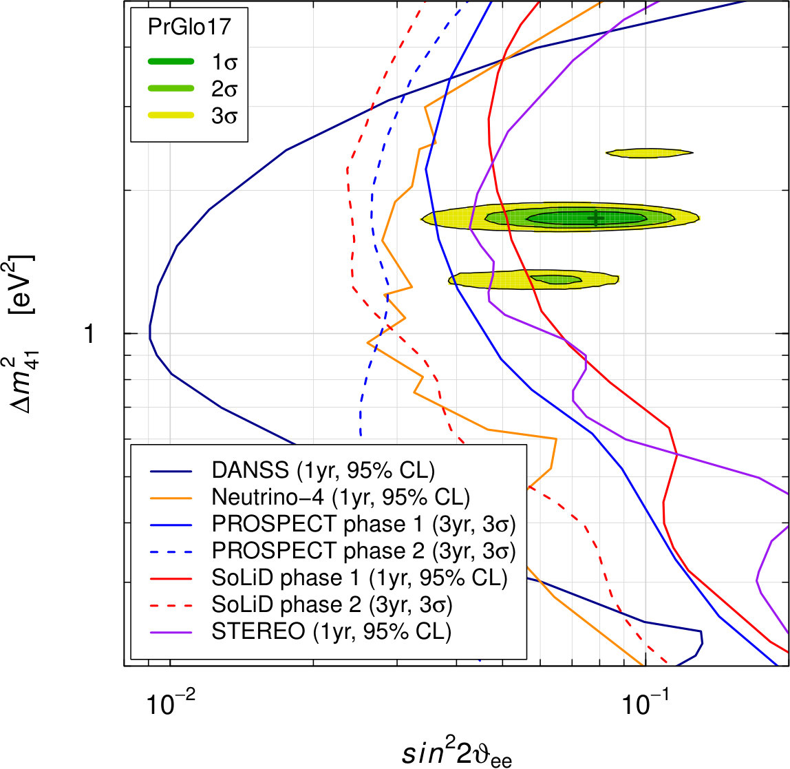 Figure 14
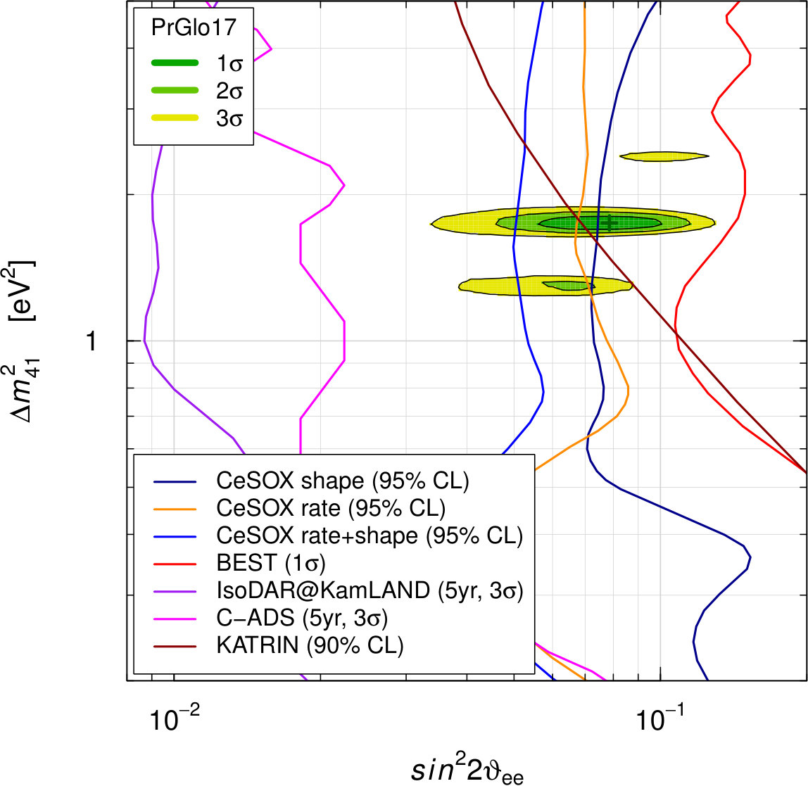 Figure 14
| Experiment | [%] | [%] | [%] | [m] | ||||||
|---|---|---|---|---|---|---|---|---|---|---|
| Bugey-4 | \rdelim}220pt[1.4] | |||||||||
| Rovno91 | ||||||||||
| Rovno88-1I | \rdelim}220pt[3.1] \rdelim}520pt[2.2] | |||||||||
| Rovno88-2I | ||||||||||
| Rovno88-1S | \rdelim}345pt[3.1] | |||||||||
| Rovno88-2S | ||||||||||
| Rovno88-2S | ||||||||||
| Bugey-3-15 | \rdelim}320pt[4.0] | |||||||||
| Bugey-3-40 | ||||||||||
| Bugey-3-95 | ||||||||||
| Gosgen-38 | \rdelim}320pt[2.0] \rdelim}420pt[3.8] | |||||||||
| Gosgen-46 | ||||||||||
| Gosgen-65 | ||||||||||
| ILL | ||||||||||
| Krasnoyarsk87-33 | \rdelim}220pt[4.1] | |||||||||
| Krasnoyarsk87-92 | ||||||||||
| Krasnoyarsk94-57 | 0 | |||||||||
| Krasnoyarsk99-34 | 0 | |||||||||
| SRP-18 | 0 | |||||||||
| SRP-24 | 0 | |||||||||
| Nucifer | 0 | |||||||||
| Chooz | 0 | |||||||||
| Palo Verde | 0 | |||||||||
| Daya Bay | 0 | |||||||||
| RENO | 0 | |||||||||
| Double Chooz | 0 |
| NDF |
| GoF |
| NDF |
| GoF |
| CL | |||
|---|---|---|---|
| 68.27% () | 0.0032 | ||
| 95.45% () | 0.018 | ||
| 99.73% () | 0.039 |
Peer Reviews
No public reviews on file for this paper yet. If you reviewed it on a platform where reviews are public (OpenReview, ICLR, NeurIPS, ICML), you can paste yours below so the community can read it here.
Videos
No videos yet. Explain this paper in a talk, walkthrough, or lecture? Add one.
aainstitutetext: Instituto de Física Corpuscular (CSIC-Universitat de València), Paterna (Valencia), Spainbbinstitutetext: INFN, Sezione di Torino, Via P. Giuria 1, I–10125 Torino, Italyccinstitutetext: Dipartimento di Fisica e Astronomia “G. Galilei”, Università di Padova, Italyddinstitutetext: INFN, Sezione di Padova, Via F. Marzolo 8, I–35131 Padova, Italyeeinstitutetext: Institute of High Energy Physics, Chinese Academy of Sciences, Beijing 100049, China
Updated Global 3+1 Analysis of Short-BaseLine Neutrino Oscillations
S. Gariazzo b
C. Giunti c,d
M. Laveder e
and Y.F. Li
Abstract
We present the results of an updated fit of short-baseline neutrino oscillation data in the framework of 3+1 active-sterile neutrino mixing. We first consider and disappearance in the light of the Gallium and reactor anomalies. We discuss the implications of the recent measurement of the reactor spectrum in the NEOS experiment, which shifts the allowed regions of the parameter space towards smaller values of . The -decay constraints of the Mainz and Troitsk experiments allow us to limit the oscillation length between about cm and m at for neutrinos with an energy of 1 MeV. The corresponding oscillations can be discovered in a model-independent way in ongoing reactor and source experiments by measuring and disappearance as a function of distance. We then consider the global fit of the data on short-baseline \hbox to0.0pt{\kern-2.5pt\overset{\scriptscriptstyle(-)}{\phantom{\nu}}\hss}{{\nu}_{\mu}}\to\hbox to0.0pt{\kern-2.5pt\overset{\scriptscriptstyle(-)}{\phantom{\nu}}\hss}{{\nu}_{e}} transitions in the light of the LSND anomaly, taking into account the constraints from \hbox to0.0pt{\kern-2.5pt\overset{\scriptscriptstyle(-)}{\phantom{\nu}}\hss}{{\nu}_{e}} and \hbox to0.0pt{\kern-2.5pt\overset{\scriptscriptstyle(-)}{\phantom{\nu}}\hss}{{\nu}_{\mu}} disappearance experiments, including the recent data of the MINOS and IceCube experiments. The combination of the NEOS constraints on and the MINOS and IceCube constraints on lead to an unacceptable appearance-disappearance tension which becomes tolerable only in a pragmatic fit which neglects the MiniBooNE low-energy anomaly. The minimization of the global in the space of the four mixing parameters , , , and leads to three allowed regions with narrow widths at . The effective amplitude of short-baseline \hbox to0.0pt{\kern-2.5pt\overset{\scriptscriptstyle(-)}{\phantom{\nu}}\hss}{{\nu}_{\mu}}\to\hbox to0.0pt{\kern-2.5pt\overset{\scriptscriptstyle(-)}{\phantom{\nu}}\hss}{{\nu}_{e}} oscillations is limited by at . The restrictions of the allowed regions of the mixing parameters with respect to our previous global fits are mainly due to the NEOS constraints. We present a comparison of the allowed regions of the mixing parameters with the sensitivities of ongoing experiments, which show that it is likely that these experiments will determine in a definitive way if the reactor, Gallium and LSND anomalies are due to active-sterile neutrino oscillations or not.
1 Introduction
Neutrino physics is a powerful probe of new physics beyond the Standard Model. The LSND Athanassopoulos:1995iw ; Aguilar:2001ty , Gallium Abdurashitov:2005tb ; Laveder:2007zz ; Giunti:2006bj ; Giunti:2010zu ; Giunti:2012tn and reactor Mention:2011rk anomalies are intriguing indications in favor of the existence of light sterile neutrinos connected with low-energy new physics. In order to assess the viability of the light sterile neutrino hypothesis, it is necessary to perform a global fit of neutrino oscillation data which takes into account not only the LSND, Gallium and reactor anomalies, but also the data of many other experiments which constrain active-sterile neutrino mixing (see the reviews in Refs. Bilenky:1998dt ; GonzalezGarcia:2007ib ; Conrad:2012qt ; Gariazzo:2015rra ).
In this paper we consider 3+1 active-sterile neutrino mixing, in which the three standard active neutrinos , , are mainly composed of three sub-eV massive neutrinos , , and there is a sterile neutrino which is mainly composed of a fourth massive neutrino at the eV scale. This is the only allowed four-neutrino mixing scheme after the demise of the 2+2 scheme Maltoni:2004ei and the fact that the 1+3 scheme with three massive neutrinos at the eV scale is strongly disfavored by cosmological measurements Ade:2015xua and by the experimental bounds on neutrinoless double- decay if massive neutrinos are Majorana particles (see Refs. Bilenky:2014uka ; DellOro:2016tmg ). We do not consider neutrino mixing schemes with more than one sterile neutrino, which are not necessary to explain the current data (see the discussions in Refs. Gariazzo:2015rra ; Giunti:2015mwa ).
In the framework of 3+1 active-sterile mixing, short-baseline (SBL) experiments are sensitive only to the oscillations generated by the squared-mass difference , with , that is much larger than the the solar squared-mass difference and the atmospheric squared-mass difference , which generate the observed solar, atmospheric and long-baseline neutrino oscillations explained by the standard three-neutrino mixing (see Refs. Capozzi:2016rtj ; Esteban:2016qun ). The 3+1 active-sterile mixing scheme is a perturbation of the standard three-neutrino mixing in which the unitary mixing matrix is extended to a unitary mixing matrix with . The effective oscillation probabilities of the flavor neutrinos in short-baseline experiments are given by Bilenky:1996rw
[TABLE]
where , is the source-detector distance and is the neutrino energy. The short-baseline oscillation amplitudes depend only on the absolute values of the elements in the fourth column of the mixing matrix:
[TABLE]
Hence, the transition probabilities of neutrinos and antineutrinos are equal and it is not possible to measure in short-baseline experiments any CP-violating effect generated by the complex phases in the mixing matrix111CP violating effects due to active-sterile neutrino mixing can, however, be observed in long-baseline deGouvea:2014aoa ; Klop:2014ima ; Berryman:2015nua ; Gandhi:2015xza ; Palazzo:2015gja ; Agarwalla:2016mrc ; Agarwalla:2016xxa ; Choubey:2016fpi ; Agarwalla:2016xlg ; Capozzi:2016vac and solar Long:2013hwa neutrino experiments. .
In this paper we update the analysis of short-baseline neutrino oscillation data Giunti:2012tn ; Giunti:2012bc ; Giunti:2013aea ; Gariazzo:2015rra revising the analysis of the rates measured in reactor neutrino experiments according to Ref. Giunti:2016elf and taking into account the recent measurements of the MINOS MINOS:2016viw , IceCube TheIceCube:2016oqi , and NEOS Ko:2016owz experiments. The MINOS and IceCube constraints on and disappearance are expected Giunti:2016oan to disfavor the low-–high- and the low-–high- parts of the allowed region that we found in our previous analyses Giunti:2012tn ; Giunti:2012bc ; Giunti:2013aea ; Gariazzo:2015rra , as was found in the 3+1 global fit presented in Ref. Collin:2016aqd , which updated Ref. Collin:2016rao with the addition of the IceCube data. The NEOS Ko:2016owz collaboration measured the spectrum of reactor ’s at a distance of 24 m and normalized their data to the Daya Bay spectrum An:2016srz measured at the large distance of about 550 m, where short-baseline oscillations are averaged out. Analyzing this normalized spectrum with short-baseline oscillations they found the best fit at and , with a which is lower by 6.5 with respect to the standard case of three-neutrino mixing without short-baseline oscillations. This is a indication in favor of short-baseline oscillations and it is intriguing to note that the best-fit value of is close to the best-fit value found in our previous global analysis of short-baseline data Gariazzo:2015rra , , albeit with a larger . However, as one can see from Table 5 of Ref. Gariazzo:2015rra , the lower bound of the allowed range of was 0.046, which is below the NEOS best-fit value. Hence, the NEOS data are not incompatible with the global indications of short-baseline oscillations and we expect that their inclusion in the fit will lead to a shift of the allowed region towards smaller values of and, consequently, of .
It is well known Okada:1996kw ; Bilenky:1996rw ; Kopp:2011qd ; Giunti:2011gz ; Giunti:2011hn ; Giunti:2011cp ; Conrad:2012qt ; Archidiacono:2012ri ; Archidiacono:2013xxa ; Kopp:2013vaa ; Giunti:2013aea ; Gariazzo:2015rra that the global fits of short-baseline data are affected by the so-called “appearance-disappearance” tension which is present Giunti:2015mwa for any number of sterile neutrinos in 3+ mixing schemes which are perturbations of the standard three-neutrino mixing required for the explanation of the observation of solar, atmospheric and long-baseline neutrino oscillations (see Refs. Capozzi:2016rtj ; Esteban:2016qun ). We expect that the inclusion in the global fit of the recent measurements of the MINOS MINOS:2016viw , IceCube TheIceCube:2016oqi , and NEOS Ko:2016owz experiment will increase somewhat the appearance-disappearance tension. In Ref. Giunti:2013aea we proposed a “pragmatic approach” in which the appearance-disappearance tension is alleviated by excluding from the global fit the low-energy bins of the MiniBooNE experiment AguilarArevalo:2008rc ; Aguilar-Arevalo:2013pmq which have an anomalous excess of -like events that is under investigation in the MicroBooNE experiment at Fermilab Gollapinni:2015lca . In this paper we will discuss the effect of MINOS, IceCube and NEOS data on the appearance-disappearance tension and how much it is alleviated in the pragmatic approach.
The plan of the paper is as follows. In section 2 we consider the experimental data on short-baseline and disappearance, motivated by the Gallium and reactor anomalies. In section 3 we consider the global fit of appearance and disappearance data, which is motivated by the addition of the LSND anomaly to the Gallium and reactor anomalies. We draw our conclusions in section 4.
2 and disappearance
In this section we consider only the experimental data on short-baseline and disappearance, which include the Gallium neutrino anomaly Abdurashitov:2005tb ; Laveder:2007zz ; Giunti:2006bj ; Giunti:2010zu ; Giunti:2012tn and the reactor antineutrino anomaly Mention:2011rk . First, we discuss in subsection 2.1 our evaluation of the reactor antineutrino anomaly by considering the updated results of the reactor rates measured in several reactor neutrino experiments. In subsection 2.2 we add the constraints of the spectra measured in the old Bugey-3 experiment Declais:1995su and in the recent NEOS experiment Ko:2016owz . Finally, in subsection 2.3 we present our results for the combined fit of reactor and Gallium data and for the global fit of all the and disappearance data.
2.1 Reactor rates
The reactor neutrino experiments which measured the absolute antineutrino flux that are considered in our analysis222We do not consider the still preliminary data of the Neutrino-4 experiment Serebrov:2017nxa .
are listed in Table 1. For each experiment labeled with the index , we listed the corresponding four fission fractions , the ratio of measured and predicted rates , the corresponding relative experimental uncertainty , the relative uncertainty which is correlated in each group of experiments indicated by the braces, and the relative theoretical uncertainty which is correlated among all the experiments. The ratios and the uncertainties and are the same as those in Ref. Giunti:2016elf . In the following we repeat for convenience333We also correct, in Table 1, the misprints of the Rovno88 correlations in Tab. 2 of Ref. Giunti:2016elf .
their derivation and we explain the derivation of the relative theoretical uncertainty .
The ratios of measured and predicted rates of the short-baseline experiments Bugey-4 Declais:1994ma , Rovno91 Kuvshinnikov:1990ry , Bugey-3 Declais:1995su , Gosgen Zacek:1986cu , ILL Kwon:1981ua ; Hoummada:1995zz , Krasnoyarsk87 Vidyakin:1987ue , Krasnoyarsk94 Vidyakin:1990iz ; Vidyakin:1994ut , Rovno88 Afonin:1988gx , and SRP Greenwood:1996pb have been calculated by the Saclay group in Ref. Mention:2011rk . The calculation of the , , and antineutrino fluxes was subsequently improved by P. Huber in Huber:2011wv . We took into account this correction with the following rescaling of the Saclay ratios444The missing index corresponds to the Krasnoyarsk99-34 experiment discussed below. :
[TABLE]
where and are, respectively, the Saclay Mention:2011rk and Saclay+Huber Huber:2011wv cross sections per fission given in Tab. 2. The index indicates the four fissionable isotopes , , , and which constitute the reactor fuel.
We considered the Krasnoyarsk99-34 experiment Kozlov:1999ct that was not considered in Refs. Mention:2011rk ; Zhang:2013ela , by rescaling the value of the corresponding experimental cross section per fission in comparison with the Krasnoyarsk94-57 result. For the long-baseline experiments Chooz Apollonio:2002gd and Palo Verde Boehm:2001ik , we applied the rescaling in Eq. (3) with the ratios given in Ref. Zhang:2013ela , divided by the corresponding survival probability caused by . For Nucifer Boireau:2015dda , Daya Bay An:2016srz , RENO RENO-AAP2016 , and Double Chooz555Double Chooz Collaboration, Private Communication. we use the ratios provided by the respective experimental collaborations.
The experimental uncertainties and their correlations listed in Table 1 have been obtained from the corresponding experimental papers. In particular:
- •
The Bugey-4 and Rovno91 experiments have a correlated 1.4% uncertainty, because they used the same detector Declais:1994ma .
- •
The Rovno88 experiments have a correlated 2.2% reactor-related uncertainty Afonin:1988gx . In addition, each of the two groups of integral (Rovno88-1I and Rovno88-2I) and spectral (Rovno88-1S, Rovno88-2S, and Rovno88-3S) measurements have a correlated 3.1% detector-related uncertainty Afonin:1988gx .
- •
The Bugey-3 experiments have a correlated 4.0% uncertainty obtained from Tab. 9 of Declais:1994ma .
- •
The Gosgen and ILL experiments have a correlated 3.8% uncertainty, because they used the same detector Zacek:1986cu . In addition, the Gosgen experiments have a correlated 2.0% reactor-related uncertainty Zacek:1986cu .
- •
The 1987 Krasnoyarsk87-33 and Krasnoyarsk87-92 experiments have a correlated 4.1% uncertainty, because they used the same detector at 32.8 and 92.3 m from two reactors Vidyakin:1987ue . The Krasnoyarsk94-57 experiment was performed in 1990-94 with a different detector at 57.0 and 57.6 m from the same two reactors Vidyakin:1990iz . The Krasnoyarsk99-34 experiment was performed in 1997-99 with a new integral-type detector at 34 m from the same reactor of the Krasnoyarsk87-33 experiment Kozlov:1999cs . There may be reactor-related uncertainties correlated among the four Krasnoyarsk experiments, but, taking into account the time separations and the absence of any information, we conservatively neglected them.
- •
Following Ref. Zhang:2013ela , we considered the two SRP measurements as uncorrelated, because the two measurements would be incompatible with the correlated uncertainty estimated in Ref. Greenwood:1996pb .
For each experiment labeled with the index , the relative theoretical uncertainty in Table 1 is given by
[TABLE]
where is the covariance matrix of the cross sections per fission of the four fissionable isotopes given in Tab. 3. In this covariance matrix, is uncorrelated from the other cross sections per fission and the corresponding uncertainty is that given in Ref. Mention:2011rk (we neglected the correlation due to the cross section uncertainty, which is of the order of ). The other three cross sections per fission have been calculated using the Huber Huber:2011wv antineutrino fluxes which have been obtained by inverting the spectra of the electrons emitted by the decays of the products of the thermal fission of , , and which have been measured at ILL in the 80’s Schreckenbach:1985ep ; Hahn:1989zr ; Haag:2014kia . As explained in Ref. Huber:2011wv , the values of the three antineutrino fluxes are correlated. We calculated the uncertainties and correlations of , , and using the information given in Ref. Huber:2011wv . The square roots of the diagonal elements of the covariance matrix in Tab. 3 give the uncertainties of the cross sections per fission reported in Tab. 2. One can see that the uncertainties of , , and are slightly larger than those calculated by Saclay group in Ref. Mention:2011rk .
Let us note that after the discovery of the unexpected “5 MeV bump” in the spectrum of the RENO RENO:2015ksa , Double Chooz Abe:2014bwa , and Daya Bay An:2015nua experiments it is believed Huber:2016fkt ; Hayes:2016qnu that the theoretical uncertainties of the reactor antineutrino fluxes may be larger than those calculated in Refs. Mueller:2011nm ; Huber:2011wv . However, since there is no well-motivated quantitative estimation of how much the theoretical uncertainties should be increased, we are compelled to use the uncertainties calculated in Refs. Mueller:2011nm ; Huber:2011wv .
Figure 1 shows the experimental ratios as functions of the reactor-detector distance . The horizontal band shows the average ratio and its uncertainty,
[TABLE]
which has been obtained by summing in quadrature the experimental and theoretical uncertainties. Hence, the reactor antineutrino anomaly is at the level of about .
The slight difference of the value of in Eq. (5) with respect to our previous estimates in Refs. Giunti:2012tn ; Gariazzo:2015rra is due to the following three changes in our analysis:
The revaluation Giunti:2016elf of the experimental ratios listed in Table 1. 2. 2.
The new treatment of the theoretical uncertainties according to Eq. (4) instead of considering an unrealistic common 2.0% Mention:2011rk . 3. 3.
The new data of the Nucifer, Daya Bay, RENO and Double Chooz experiments and the consideration for the first time of the Krasnoyarsk99-34 experiment.
The reactor antineutrino anomaly can be explained in the framework of 3+1 neutrino mixing through neutrino oscillations generated by the effective mixing angle , which determines the survival probability of ’s and ’s according to Eq. (1). The result of the fit of the reactor rates are given in the first column of Table 4 and in Fig. 2, where we have drawn the allowed regions in the – plane.
From Fig. 2 one can see that the allowed region666In all the paper we consider allowed regions at , , and , which correspond, respectively, to 68.27%, 95.45%, and 99.73% confidence level. The allowed regions in two-parameter planes are drawn considering two degrees of freedom, which correspond, respectively, to , , and from the minimum .
in the – plane is at a rather low value of , but the allowed regions at and extend to higher values of , without an upper bound. The favorite values of the amplitude of -disappearance oscillations are around 0.1, but the allowed region in the – plane covers the range , which corresponds to .
Table 4 gives the difference between the of no oscillations and , and the corresponding number of ’s for the two degrees of freedom corresponding to the two fitted parameters and . The case of no oscillations turns out to be disfavored at the level of .
2.2 Reactor spectra
In our previous analyses Giunti:2012tn ; Giunti:2012bc ; Giunti:2013aea ; Gariazzo:2015rra we considered the ratio of the spectra measured at 40 m and 15 m from the source in the Bugey-3 experiment Declais:1995su . These data provide robust information on short-baseline disappearance, which is independent of any theoretical calculation of the spectrum and of the solution of the “5 MeV bump” problem mentioned in subsection 2.1.
In this paper we add the constraints obtained in the recent NEOS experiment by taking into account the corresponding to Fig. 4 of Ref. Ko:2016owz , which has been kindly provided to us by the NEOS Collaboration777NEOS Collaboration, Private Communication.. The NEOS constraints are mostly independent of theoretical calculations of the spectrum and of the solution of the “5 MeV bump” problem, because the NEOS has been obtained by fitting the NEOS spectrum normalized to the Daya Bay spectrum An:2016srz measured at the large distance of about 550 m, where the short-baseline oscillations due to are averaged out. A small dependence on the theoretical calculation of the spectrum Mueller:2011nm ; Huber:2011wv comes from the corrections due to the differences of the fission fractions of the NEOS and Daya Bay reactors An:2016srz ; Ko:2016owz and a small dependence on the “5 MeV bump” problem comes from a possible dependence of the “5 MeV bump” on the different fission fractions of NEOS and Daya Bay Huber:2016xis . We neglect these possible small effects.
The results of the fit of the Bugey-3 and NEOS spectra are given in the second column of Table 4 and in Fig. 2, where one can see that the NEOS constraints are dominating. There are closed allowed islands at which are determined mainly by the NEOS data and the best-fit values of the oscillation parameters in Table 4 correspond to the best fit reported in Ref. Ko:2016owz . Hence, the NEOS constraints can be interpreted as a weak indication in favor of short-baseline oscillations which may be compatible with the reactor antineutrino anomaly based on the reactor rates discussed in subsection 2.1. This is confirmed by the disfavoring of the case of no oscillations at the level of , as shown in Table 4.
The third column of Table 4 and Fig. 3 show the results of the combined fit of the rate and spectral data of reactor antineutrino experiments. As reported in Table 4, the combined fit disfavors the case of no oscillations at the level of , which is about the same level obtained from the analysis of the reactor rates alone. Hence, the NEOS constraints do not exclude the reactor antineutrino anomaly. However, in spite of the weak NEOS indication in favor of short-baseline oscillations discussed above, the statistical significance of the anomaly does not increase by including the NEOS data because there is a mild tension with the reactor rates which is illustrated by the contours in Fig. 3. Indeed, the rates-spectra parameter goodness-of-fit is only ().
2.3 Global and disappearance
In this subsection we discuss the combination of the reactor data with the data of the Gallium neutrino anomaly, other and disappearance data and the -decay constraints of the Mainz Kraus:2012he and Troitsk Belesev:2012hx ; Belesev:2013cba experiments.
The fourth column of Table 4 and Fig. 3 show the results of the combined fit of reactor and Gallium data. Since both sets of data indicate short-baseline and disappearance, the statistical significance of active-sterile neutrino oscillations increases to and the allowed regions in the – plane are confined to and .
Besides the reactor and Gallium data, short-baseline disappearance888We work in the framework of a local quantum field theory in which the CPT symmetry implies that the survival probabilities of neutrinos and antineutrinos are equal (see Ref. Giunti:2007ry ).
is constrained by solar and KamLAND neutrino data Giunti:2009xz ; Palazzo:2011rj ; Palazzo:2012yf ; Giunti:2012tn ; Palazzo:2013me , by the KARMEN Armbruster:1998uk and LSND Auerbach:2001hz scattering data Conrad:2011ce ; Giunti:2011cp and by the T2K near detector constraints Abe:2014nuo .
We updated our 2012 solar+KamLAND constraint Giunti:2012tn by including the latest solar data: the new results from the fourth phase of the Super-Kamiokande experiment Abe:2016nxk and the final results of Borexino phase-I Bellini:2013lnn . We also updated the KamLAND data analysis by using the Saclay+Huber cross sections per fission Giunti:2016elf . Finally, we used the updated value of in the 2016 Review of Particle Physics Olive:2016xmw . We obtained the new marginal shown in Fig. 4, where it is confronted with the old one obtained in Ref. Giunti:2012tn . The new solar+KamLAND constraint is weaker than the 2012 one because of the larger Saclay+Huber reactor rate prediction used in the analysis of KamLAND data and because the new value of is smaller than that in 2012.
The results of the combined analysis of all and disappearance data are shown in the fifth column of Table 4 and Fig. 5. Since the analysis of solar+KamLAND, -, and T2K data do not show any indication of short-baseline disappearance, the combination with the reactor and Gallium data shifts the allowed regions in the – plane in Fig. 5 to smaller values of with respect to Fig. 3: . On the other hand, the range of in Figs. 3 and 5 is similar, with the lower bound and no upper bound.
Large values of can be constrained with the data of -decay experiments (see Ref. Gariazzo:2015rra ). As in Ref. Giunti:2012bc , we use the -decay constraints of the Mainz Kraus:2012he and Troitsk Belesev:2012hx ; Belesev:2013cba experiments, which give the allowed regions in the – plane shown in Fig. 5. One can see that the allowed regions are confined to the range
[TABLE]
For the oscillation length we have
[TABLE]
This is a range of oscillation lengths which can be explored in a model independent way in the new short-baseline reactor neutrino experiments (DANSS Alekseev:2016llm , Neutrino-4 Serebrov:2017nxa , PROSPECT Ashenfelter:2015uxt , SoLid Michiels:2016qui , STEREO Manzanillas:2017rta ) and in the SOX Borexino:2013xxa and BEST Barinov:2016znv radioactive source experiments by measuring the reactor antineutrino rate as a function of distance. However, they will need to be sensitive to small oscillations with the amplitude
[TABLE]
Figure 6 shows the sensitivities of the short-baseline reactor antineutrino experiments DANSS Alekseev:2016llm , Neutrino-4 Serebrov:2012sq , PROSPECT Ashenfelter:2015uxt , SoLid Ryder:2015sma , and STEREO Helaine:2016bmc in comparison with the allowed regions in the – plane in Fig. 5. One can see that they will cover most of the allowed regions for and not too small . Figure 6 shows the sensitivities of the CeSOX Borexino:2013xxa and BEST Barinov:2016znv source experiments, of IsoDAR@KamLAND Abs:2015tbh and C-ADS Ciuffoli:2015uta , and of the KATRIN Drexlin-NOW2016 ) electron neutrino mass experiment999See also the studies in Refs. Riis:2010zm ; Formaggio:2011jg ; SejersenRiis:2011sj ; Esmaili:2012vg . There are also promising possibilities to observe the effects of eV-scale neutrinos in Holmium electron-capture experiments Gastaldo:2016kak . . The source experiments will cover the large- parts of the allowed regions, the IsoDAR@KamLAND and C-ADS experiments can cover almost all the allowed regions, except the large- part and the small-–small- parts, and KATRIN will cover the large- part. Hence, there are favorable perspectives for a definitive solution of the short-baseline \hbox to0.0pt{\kern-2.5pt\overset{\scriptscriptstyle(-)}{\phantom{\nu}}\hss}{{\nu}_{e}} disappearance problem in the near future.
3 Fits of appearance and disappearance data
In this section we present the results of 3+1 fits of short-baseline neutrino oscillation data which include and appearance data and and disappearance data, in addition to the and disappearance data considered in section 2. Our fits are based on a analysis in the four-dimensional space of the mixing parameters , , , and .
We consider the following short-baseline and appearance data: the LSND signal in favor of transitions Athanassopoulos:1995iw ; Aguilar:2001ty , the data of the MiniBooNE AguilarArevalo:2008rc ; Aguilar-Arevalo:2013pmq experiment, and the constraints of the BNL-E776 Borodovsky:1992pn , KARMEN Armbruster:2002mp , NOMAD Astier:2003gs , ICARUS Antonello:2013gut and OPERA Agafonova:2013xsk experiments.
There is no indication in favor of short-baseline and disappearance from any experiment. Therefore, the current and disappearance data lead to constraints on . We consider the constraints obtained from the CDHSW experiment Dydak:1983zq , from the analysis Maltoni:2007zf of the data of atmospheric neutrino oscillation experiments, from the analysis of the SciBooNE-MiniBooNE neutrino Mahn:2011ea and antineutrino Cheng:2012yy data, which were included in our previous fits Giunti:2013aea ; Gariazzo:2015rra ; Giunti:2016oan . In addition, we take into account the recent data of the MINOS MINOS:2016viw and IceCube TheIceCube:2016oqi experiments. The MINOS constraint was easily included in our numerical computation by using the ROOT program in the MINOS data release101010http://www-numi.fnal.gov/PublicInfo/forscientists.html , which computes the for input values of the 3+1 mixing parameters. On the other hand, we had to calculate the IceCube , as described in the following subsection 3.1.
3.1 Analysis of IceCube data
The IceCube detector measures the incoming (anti)muons generated by the interaction of atmospheric muon (anti)neutrinos with the surrounding earth and ice, as a function of the neutrino energy and of the zenith angle. For high-energy, up-going atmospheric neutrinos that reach the detector after having crossed the Earth, the ratio is of the same order of that in SBL experiments. In this case, the oscillations arising from the usual atmospheric and solar squared mass differences have a very long wavelength and can be neglected, but the SBL squared mass difference plays an active role. The sterile neutrino influence on the observed flux is given by the matter effects that modify the oscillation patterns inside the Earth. This happens because the matter potential is different for the different active neutrino flavors, for which the charged and neutral current interactions are not the same GonzalezGarcia:2005xw , and there is no potential for the sterile neutrinos.
We use the 20,145 released IceCube events in the approximate energy range between 320 GeV and 20 TeV, detected over 343.7 days in the 86-strings configuration Aartsen:2015rwa for constraining the active-sterile mixing parameters. The 99.9% of the IceCube events is expected to come from neutrino-induced muon events, where the neutrinos originate from the decays of atmospheric pions and kaons. The contribution from charmed meson decays is negligible Aartsen:2014muf ; Aartsen:2015rwa .
The calculation of the contribution from IceCube is divided into three parts: the calculation of the theoretical flux for each set of mixing parameters, for which one needs to propagate the atmospheric neutrinos through the Earth, the estimate of the expected number of events in the detector, for which we use the IceCube Monte Carlo data, and finally the computation of the , obtained comparing theoretical and observed events. For all these parts we use the data111111http://icecube.wisc.edu/science/data/IC86-sterile-neutrino/ and we follow the prescriptions presented in Ref. TheIceCube:2016oqi .
To obtain the predicted neutrino flux at the detector, we use the -SQuIDS code121212http://github.com/Arguelles/nuSQuIDS, a C++ package based on the Simple Quantum Integro-Differential Solver (SQuIDS)131313http://github.com/jsalvado/SQuIDS Delgado:2014kpa , that contains all the necessary tools to numerically solve the master equation that rules the neutrino evolution in the Earth GonzalezGarcia:2005xw .
The initial flux we consider is the unoscillated HKKM flux Honda:1995hz ; Honda:2004yz ; Sanuki:2006yd ; Honda:2006qj with the H3a knee correction Gaisser:2013bla , that we use for obtaining the initial spectrum of neutrinos from pion and kaon decays. This model is usually referred to as the “Honda-Gaisser” model. We do not employ here the other six atmospheric flux variants that are considered in Ref. TheIceCube:2016oqi , but we tested that our results do not change significantly if another model is used instead of the Honda-Gaisser one. Since our analysis is based not only on the IceCube data, our final result would be almost unaffected.
The unoscillated flux is propagated inside the Earth with the -SQuIDS code, which uses the Preliminary Reference Earth Model Dziewonski:1981xy for the inner density profile of the Earth. For the neutrino-matter interactions, the charged current cross section is dominated by deep inelastic scattering, which involves neutrino-nucleon scattering. The main uncertainty in this case is in the parton distribution functions. In the -SQuIDS code, the perturbative QCD calculation in Refs. Arguelles:2015wba are used for the neutrino-nucleon cross-section calculation. We do not treat the uncertainties on the Earth density profile and on the deep inelastic scattering cross section.
The full expression for the (anti)neutrino flux at the detector is given by TheIceCube:2016oqi (see also Refs. Arguelles:2015a ; Jones:2015bya )
[TABLE]
Here, is the zenith angle and the energy of the incoming (anti)neutrino, while is the oscillated (anti)neutrino flux from pion (kaon) decays. The free parameters in the above equation are: the neutrino and antineutrino flux normalizations, and ; the pion-to-kaon ratio, ; the spectral index correction, . These are treated as continuous nuisance parameters in our analysis, as explained in Ref. TheIceCube:2016oqi . The pivot energy is fixed to be approximately near the median of the energy distribution of the measured events, being TeV.
The function parameterizes the atmospheric density uncertainties. This function is assumed to be linear and it is obtained by imposing the AIRS constraints on the atmospheric temperature141414https://climatedataguide.ucar.edu/climate-data/airs-and-amsu-tropospheric-air-temperature-and-specific-humidity. The expression reads as Arguelles:2015a :
[TABLE]
where GeV, TeV, and . The parameter represents the last one of our nuisance parameters.
The theoretical flux is converted into a number of expected events using the Monte Carlo (MC) data released by the IceCube collaboration TheIceCube:2016oqi . The MC data are needed to model the detector capabilities to measure the incoming events as a function of the real energy and zenith angle of the muon (anti)neutrino, and of the corresponding quantities for the reconstructed (anti)muon event. For each combination of mixing and nuisance parameters, we use the MC data to convert the obtained theoretical flux into the expected number of events that we compare with the data as explained below. Since IceCube cannot distinguish a muon from an antimuon, neutrinos and antineutrinos events are summed up together. It is however important to treat properly both the components, since the matter oscillation patterns for neutrinos and antineutrinos are different, with the consequence that the disappearance of neutrinos and antineutrinos is not the same.
We build our using a binned Poissonian likelihood, written as
[TABLE]
where represents the number of observed events in the bin and the corresponding number of expected events as a function of the model parameters , that includes both mixing and nuisance parameters. Following Ref. TheIceCube:2016oqi , we consider a grid with 10 logarithmic bins in the reconstructed energy, with , and 21 linear bins for the cosine of the reconstructed zenith angle, in the range .
For each combination of the mixing parameters, we minimize the over the five nuisance parameters described above (, , , , ). We adopt a standard Nelder-Mead algorithm for the minimization Nelder:1965a . It is important to note that for each point in the mixing parameter space we needed to minimize independently over the nuisance parameters. We checked that the preferred values of the nuisance parameters do not vary significantly outside the adopted Gaussian priors TheIceCube:2016oqi .
We show in Fig. 7 the comparison of the official IceCube 90% and 99% CL exclusion curves in the – plane for TheIceCube:2016oqi with our results. In our analysis of IceCube data we do not vary the efficiency of the Digital Optical Modules because we do not have sufficient information. Despite this fact, one can see from Fig. 7 that the results of our analysis are in good agreement with those of the IceCube collaboration. Moreover, we emphasize that the IceCube data are just one of the datasets in our global analyses, and small differences in the IceCube analysis do not play a significant role when computing the global fit.
Since the calculation of the given a set of mixing parameters is a highly demanding computational task, it is impossible to directly include the code that calculates the of the IceCube data in our complete fitting routine without slowing it down in an unacceptable way. Therefore, we adopted the following method. Since we are more interested in scanning the region near the expected 3+1 mixing best-fit, we employed the results of the 3+1 fit of SBL data without IceCube in order to generate with a Markov Chain Monte Carlo (MCMC) 3,000 random points whose distribution covers an area of the parameter space around the expected best-fit region. In order to cover the rest of the full four-dimensional parameter space (; , , ), we generated uniformly 21,000 more random points. We end up with a set P of 24,000 points for which we computed the IceCube in an affordable time. In the complete fitting routine, we computed the IceCube contribution to the in each point in the full four-dimensional parameter space with a linear interpolation of the ’s of the nearest points in the set P obtained with a Delaunay triangulation.
3.2 Fit of the 2016 data set without MINOS and IceCube
In this subsection we present the results of the 3+1 global fit “Glo16A” of the appearance and disappearance SBL data available in 2016151515We consider all the and disappearance data discussed in section 2, with the exceptions of the T2K near detector constraints Abe:2014nuo on , which unfortunately cannot be included in the global fit because they have been obtained under the assumption , and of the Mainz Kraus:2012he and Troitsk Belesev:2012hx ; Belesev:2013cba -decay constraints, which are not needed because the value of is constrained within a few by the combination of appearance and disappearance data. , except MINOS MINOS:2016viw and IceCube TheIceCube:2016oqi , which will be added in subsection 3.3 in order to clarify their effects on the results of the analysis. In the Glo16A fit we also do not take into account the NEOS Ko:2016owz data which have been available to us in the beginning of 2017 and will be considered in subsection 3.4.
The results of the Glo16A fit are shown by the first column of Tab. 5, by Fig. 8, and by the solid purple curves in Fig. 9, which gives the marginal as a function of the mixing parameters , , and , from which one can obtain the corresponding marginal allowed intervals at different confidence levels.
The global goodness of fit of is acceptable, but there is a relevant appearance-disappearance tension quantified by a parameter goodness of fit of . If one is willing to accept such appearance-disappearance tension, one can adopt the allowed regions of the oscillation parameters shown in Fig. 8.
The Glo16A fit is an update of the GLO fit presented in Ref. Gariazzo:2015rra , with a similar set of data. It can also be compared with the global fit in Ref. Collin:2016rao , where a similar set of data was considered. With respect to Ref. Collin:2016rao , we find larger allowed regions for and we do not have the allowed region at found in Ref. Collin:2016rao at 99% CL. However, there is an approximate agreement of our results with those of Ref. Collin:2016rao , with a remarkable closeness of the best-fit point in the mixing parameter space.
3.3 Effects of MINOS and IceCube
In this subsection we present the 3+1 global fit “Glo16B” with the addition of the 2016 data of the MINOS MINOS:2016viw and IceCube TheIceCube:2016oqi experiments. The results are shown by the second column of Tab. 5, by Fig. 10, and by the solid blue curves in Fig. 9.
Comparing Fig. 10 with Fig. 8, one can see that the addition of the MINOS and IceCube data leads to the exclusion of the low-–high- part of the allowed region, as expected (see the discussion in section 1). On the other hand, the high-–low- part of the allowed region is practically unaffected by the MINOS and IceCube constraints. As a consequence, also the low-–high- part of the allowed region in Fig. 8 is excluded in Fig. 10, whereas the high-–low- part of the allowed region is practically unaffected.
From Tab. 5 one can see that including the MINOS and IceCube data increases the appearance-disappearance tension by lowering the parameter goodness of fit from to . This is a consequence of the reduction of the upper limit of the allowed range of in the Glo16B fit with respect to the Glo16A fit shown in Fig. 9.
Figure 11 shows the effect of adding to the data set of the Glo16A fit the MINOS and IceCube data separately and together. One can see that the IceCube data are slightly more effective than the MINOS data in reducing the low-–high- part of the allowed region.
The MINOS and IceCube data give information not only on the 3+1 mixing parameters , , and that we have considered so far, but also on . The sensitivity to is due in MINOS to the neutral-current event sample MINOS:2016viw and in IceCube to the matter effects for high-energy neutrinos propagating in the Earth, which depend on all the elements of the mixing matrix Nunokawa:2003ep ; Choubey:2007ji ; Razzaque:2011ab ; Razzaque:2012tp ; Esmaili:2012nz ; Esmaili:2013vza ; Esmaili:2013cja ; Lindner:2015iaa . Limits on the value of have been obtained in the analyses of the atmospheric neutrino data of the Super-Kamiokande Abe:2014gda and IceCube DeepCore Aartsen:2017bap experiments, in the analysis of the data of the MINOS experiment Adamson:2010wi ; Adamson:2011ku ; MINOS:2016viw , and in the phenomenological fits in Refs. Kopp:2013vaa ; Collin:2016aqd . There is also a bound on given by the absence of a 3+1 excess of oscillations in the OPERA experiment Agafonova:2015neo .
Figure 9 shows the marginal as a function of in our Glo16B fit, from which one can see that we obtain the stringent upper bound
[TABLE]
At 90% CL we have and in the common parameterization of the unitary mixing matrix used in Ref. Collin:2016aqd . This bound on is about the same as that reported in Ref. Collin:2016aqd for . However, we do not find a 90% CL allowed region of the mixing parameters at and our bound on applies for any value of .
Figure 11 shows the correlated bounds on and that we obtain considering the MINOS and IceCube data separately and together. One can see that the IceCube data give more stringent constraints on than the MINOS data for .
3.4 Effects of NEOS
We finally consider also the NEOS Ko:2016owz data and obtain the 3+1 global fit “Glo17” which includes all data available so far in 2017. The results are shown by the third column of Tab. 5, by Fig. 12, and by the solid orange curves in Fig. 9.
Comparing Fig. 12 with Fig. 10, it is evident that the inclusion of the NEOS constraints has a dramatic effect on the allowed regions, leading to the fragmentation of the allowed region in three islands with narrow widths. The best-fit island is at . There is an island allowed at at , and an island allowed at at . Moreover, the NEOS constraints shifts the allowed range of from in the Glo16B fit to in the Glo17 fit, as shown in Fig. 9. Therefore, the appearance-disappearance tension is increased, as shown by the parameter goodness of fit in Tab. 5. Since this low value of the appearance-disappearance parameter goodness of fit is hardly acceptable, we are led to consider, in the next subsection, the “pragmatic approach” proposed in Ref. Giunti:2013aea .
3.5 Pragmatic fit
In this section we consider the “pragmatic approach” Giunti:2013aea in which the low-energy bins of the MiniBooNE experiment AguilarArevalo:2008rc ; Aguilar-Arevalo:2013pmq which have an anomalous excess of \hbox to0.0pt{\kern-2.5pt\overset{\scriptscriptstyle(-)}{\phantom{\nu}}\hss}{{\nu}_{e}}-like events are omitted from the global fit. As shown in Fig. 1b of Ref. Giunti:2016oan , the region allowed by the appearance data shifts towards larger values of and smaller values of when the MiniBooNE low-energy bins are omitted from the fit. As a result, the overlap of the appearance and disappearance allowed regions increases, relieving the appearance-disappearance tension.
One can question the scientific correctness of the data selection in the pragmatic approach, but we note that the MiniBooNE low-energy excess is widely considered to be suspicious161616Part of the MiniBooNE low-energy anomaly may be explained by taking into account nuclear effects in the energy reconstruction Martini:2012fa ; Martini:2012uc , but this effect is not sufficient to solve the problem Ericson:2016yjn .
because of the large background. Some of this background can be due to photon events which are indistinguishable from \hbox to0.0pt{\kern-2.5pt\overset{\scriptscriptstyle(-)}{\phantom{\nu}}\hss}{{\nu}_{e}} events in the MiniBooNE liquid scintillator detector. These photons can be generated by the decays of ’s produced by the neutral-current interactions of the \hbox to0.0pt{\kern-2.5pt\overset{\scriptscriptstyle(-)}{\phantom{\nu}}\hss}{{\nu}_{\mu}} beam. When only one of the two photons emitted in the decay is visible, its signal cannot be distinguished from a \hbox to0.0pt{\kern-2.5pt\overset{\scriptscriptstyle(-)}{\phantom{\nu}}\hss}{{\nu}_{e}} event in a liquid-scintillator detector. The suspicion that this photon background may be responsible for the MiniBooNE low-energy excess motivated the realization of the MicroBooNE experiment at Fermilab Gollapinni:2015lca , which is able to distinguish between photon and \hbox to0.0pt{\kern-2.5pt\overset{\scriptscriptstyle(-)}{\phantom{\nu}}\hss}{{\nu}_{e}} events by using a Liquid Argon Time Projection Chamber (LArTPC). Waiting for the results of this experiment, we think that it is reasonable to adopt the pragmatic approach of omitting from the global fit the MiniBooNE low-energy data.
The results of the pragmatic 3+1 global fit “PrGlo17”, which includes the MINOS, IceCube and NEOS data, are shown by the fourth column of Tab. 5, by Fig. 13, and by the dashed red curves in Fig. 9.
From Tab. 5 one can see that, as expected, the exclusion from the fit of the MiniBooNE low-energy data leads to an increase of the parameter goodness of fit from the unacceptable of the Glo17 fit to the acceptable of the PrGlo17 fit. There is still a mild appearance-disappearance tension, but the tolerable value of parameter goodness of fit leads us to consider the PrGlo17 fit as acceptable.
Comparing the allowed regions of the oscillation parameters in Fig. 13 for the PrGlo17 fit with those in Fig. 12 for the Glo17 fit and the corresponding marginal curves in Fig. 9, one can see that the differences are small. As a consequence of the larger overlap of the regions allowed by the fits of appearance and disappearance data, the PrGlo17 fit has a minimum significantly smaller than the Glo17 fit, which leads to an increased preference of the best-fit island at , to a small shrink of the island at , and at a significant reduction of the island at (the corresponding interval for one degree of freedom allowed by the marginal in Fig. 9 disappears).
Table 6 gives the marginal allowed intervals of the mixing parameters , , and . The stringent upper bounds on slightly improve those found in the Glo16B fit (see Eq. (12) and Fig. 9). At 90% CL we have and .
We consider the results of the PrGlo17 fit as the current status of our 3+1 analysis of short-baseline neutrino oscillation data. Figure 14 shows a comparison of the sensitivities of future experiments with the PrGlo17 allowed regions of Fig. 13 for: 14 \hbox to0.0pt{\kern-2.5pt\overset{\scriptscriptstyle(-)}{\phantom{\nu}}\hss}{{\nu}_{\mu}}\to\hbox to0.0pt{\kern-2.5pt\overset{\scriptscriptstyle(-)}{\phantom{\nu}}\hss}{{\nu}_{e}} transitions (SBN Antonello:2015lea , nuPRISM Bhadra:2014oma , JSNS2 Harada:2013yaa ); 14 \hbox to0.0pt{\kern-2.5pt\overset{\scriptscriptstyle(-)}{\phantom{\nu}}\hss}{{\nu}_{\mu}} disappearance (SBN Antonello:2015lea , KPipe Axani:2015zxa ); 14,14 \hbox to0.0pt{\kern-2.5pt\overset{\scriptscriptstyle(-)}{\phantom{\nu}}\hss}{{\nu}_{e}} disappearance (DANSS Alekseev:2016llm , Neutrino-4 Serebrov:2012sq , PROSPECT Ashenfelter:2015uxt , SoLid Ryder:2015sma , STEREO Helaine:2016bmc , CeSOX Borexino:2013xxa , BEST Barinov:2016znv IsoDAR@KamLAND Abs:2015tbh , C-ADS Ciuffoli:2015uta , KATRIN Drexlin-NOW2016 ). It is clear that these experiments will give definitive information on the existence of active-sterile short-baseline oscillations connected with the LSND, Gallium and reactor anomalies.
4 Conclusions
In this paper we updated the global fit of short-baseline neutrino oscillation data in the framework of 3+1 active-sterile neutrino mixing Giunti:2012tn ; Giunti:2012bc ; Giunti:2013aea ; Gariazzo:2015rra .
We considered first, in section 2, the data on and disappearance which include the Gallium neutrino anomaly data Abdurashitov:2005tb ; Laveder:2007zz ; Giunti:2006bj ; Giunti:2010zu ; Giunti:2012tn and the reactor antineutrino anomaly data Mention:2011rk . The resulting allowed region in the – plane is rather wide, as shown in Fig. 5, but it is smaller than that found in our previous analysis Giunti:2012tn , mainly as a result of the constraints given by the recent NEOS Ko:2016owz experiment. The allowed region obtained with neutrino oscillation data alone has no upper bound for , but it can be limited Giunti:2012bc using the constraints found in the Mainz Kraus:2012he and Troitsk Belesev:2012hx ; Belesev:2013cba -decay experiments, as shown in Fig. 5. We found the upper limit at . Hence, as shown in Fig. 6, the ongoing reactor, source and -decay experiments can clarify in a definitive way the existence of short-baseline \hbox to0.0pt{\kern-2.5pt\overset{\scriptscriptstyle(-)}{\phantom{\nu}}\hss}{{\nu}_{e}} disappearance due to active-sterile neutrino mixing.
We presented also, in section 3, the results of global fits of all the available \hbox to0.0pt{\kern-2.5pt\overset{\scriptscriptstyle(-)}{\phantom{\nu}}\hss}{{\nu}_{\mu}}\to\hbox to0.0pt{\kern-2.5pt\overset{\scriptscriptstyle(-)}{\phantom{\nu}}\hss}{{\nu}_{e}} appearance data, \hbox to0.0pt{\kern-2.5pt\overset{\scriptscriptstyle(-)}{\phantom{\nu}}\hss}{{\nu}_{\mu}} disappearance data, in addition to the \hbox to0.0pt{\kern-2.5pt\overset{\scriptscriptstyle(-)}{\phantom{\nu}}\hss}{{\nu}_{e}} disappearance data considered in section 2. We discussed the effects on the global fits of the recent data of the MINOS MINOS:2016viw , IceCube TheIceCube:2016oqi , and NEOS Ko:2016owz experiments. As expected, the MINOS, IceCube and NEOS data aggravate the appearance-disappearance tension, which becomes tolerable only in the pragmatic PrGlo17 fit discussed in subsection 3.5, which is our recommended result.
We found that, as expected Collin:2016aqd ; Giunti:2016oan , the MINOS and IceCube constraints on \hbox to0.0pt{\kern-2.5pt\overset{\scriptscriptstyle(-)}{\phantom{\nu}}\hss}{{\nu}_{\mu}} disappearance disfavor the low-–high- and the low-–high- parts of the allowed region. The addition of the NEOS data has the more dramatic effect of reducing the allowed region to three islands with narrow widths and at . The best-fit island is at . There is an island allowed at at , and an island allowed at at . However, as illustrated in Fig. 14, the ongoing and planned experiments have the possibility to cover all the allowed regions of the mixing parameters and we expect that they will reach in a few years a definitive conclusion on the existence of the short-baseline oscillations indicated by the LSND experiment and by the Gallium and reactor neutrino anomalies.
An interesting feature of the 3+1 analysis of the MINOS and IceCube data is that there is a dependence on Nunokawa:2003ep ; Choubey:2007ji ; Razzaque:2011ab ; Razzaque:2012tp ; Esmaili:2012nz ; Esmaili:2013vza ; Esmaili:2013cja ; Lindner:2015iaa . We obtained the stringent bounds on the value of given in Tab. 6, which are comparable to those obtained in Ref. Collin:2016aqd .
The determination of active-sterile neutrino mixing presented in this paper is of interest also for the phenomenology of long-baseline experiments deGouvea:2014aoa ; Klop:2014ima ; Berryman:2015nua ; Gandhi:2015xza ; Palazzo:2015gja ; Agarwalla:2016mrc ; Agarwalla:2016xxa ; Choubey:2016fpi ; Agarwalla:2016xlg ; Capozzi:2016vac , and neutrinoless double- decay experiments Barry:2011wb ; Li:2011ss ; Rodejohann:2012xd ; Giunti:2012tn ; Girardi:2013zra ; Pascoli:2013fiz ; Meroni:2014tba ; Abada:2014nwa ; Giunti:2015kza ; Pas:2015eia .
We did not consider the problem of the cosmological bounds on active-sterile neutrino mixing Ade:2015xua , which most likely must be solved with a non-standard effect as a large lepton asymmetry Hannestad:2012ky ; Mirizzi:2012we ; Saviano:2013ktj ; Hannestad:2013pha or secret interactions of the sterile neutrino mediated by a massive vector or pseudoscalar boson Hannestad:2013ana ; Dasgupta:2013zpn ; Mirizzi:2014ama ; Saviano:2014esa ; Forastieri:2015paa ; Chu:2015ipa ; Archidiacono:2016kkh , which suppress the thermalization of the sterile neutrino in the early Universe.
In conclusion, this paper gives information on what are the regions of the parameter space of 3+1 neutrino mixing which must be explored by new experiments in order to check the indications given by the LSND, Gallium and reactor anomalies. Let us emphasize the importance of an experimental confirmation of these oscillations, that would imply the existence of light sterile neutrinos. These are new particles with properties outside the realm of the Standard Model and their discovery would open a prodigious window on new low-energy physics.
Acknowledgments
We are very grateful to the NEOS Collaboration for giving us the table of corresponding to Fig. 4 of Ref. Ko:2016owz . The work of S.G. is supported by the Spanish grants FPA2014-58183-P, Multidark CSD2009-00064 and SEV-2014-0398 (MINECO), and PROMETEOII/2014/084 (Generalitat Valenciana). The work of C.G. and M.L. was partially supported by the research grant Theoretical Astroparticle Physics number 2012CPPYP7 under the program PRIN 2012 funded by the Italian Ministero dell’Istruzione, Università e della Ricerca (MIUR) and by the research project TAsP funded by the Instituto Nazionale di Fisica Nucleare (INFN). The work of Y.F.L. was supported in part by the National Natural Science Foundation of China under Grant Nos. 11305193 and 11135009, by the Strategic Priority Research Program of the Chinese Academy of Sciences under Grant No. XDA10010100, by the CAS Center for Excellence in Particle Physics (CCEPP).
The reference list from the paper itself. Each links out to its DOI / PubMed record.
- 1(1) LSND collaboration, C. Athanassopoulos et al., Candidate events in a search for ν ¯ μ → ν ¯ e → subscript ¯ 𝜈 𝜇 subscript ¯ 𝜈 𝑒 \bar{\nu}_{\mu}\to\bar{\nu}_{e} oscillations , Phys. Rev. Lett. 75 (1995) 2650–2653, [ nucl-ex/9504002 ].
- 2(2) LSND collaboration, A. Aguilar et al., Evidence for neutrino oscillations from the observation of ν ¯ e subscript ¯ 𝜈 𝑒 \bar{\nu}_{e} appearance in a ν ¯ μ subscript ¯ 𝜈 𝜇 \bar{\nu}_{\mu} beam , Phys. Rev. D 64 (2001) 112007, [ hep-ex/0104049 ].
- 3(3) SAGE collaboration, J. N. Abdurashitov et al., Measurement of the response of a Ga solar neutrino experiment to neutrinos from an Ar-37 source , Phys. Rev. C 73 (2006) 045805, [ nucl-ex/0512041 ].
- 4(4) M. Laveder, Unbound neutrino roadmaps , Nucl. Phys. Proc. Suppl. 168 (2007) 344–346 . · doi ↗
- 5(5) C. Giunti and M. Laveder, Short-Baseline Active-Sterile Neutrino Oscillations? , Mod. Phys. Lett. A 22 (2007) 2499–2509, [ hep-ph/0610352 ].
- 6(6) C. Giunti and M. Laveder, Statistical Significance of the Gallium Anomaly , Phys. Rev. C 83 (2011) 065504, [ ar Xiv:1006.3244 ].
- 7(7) C. Giunti, M. Laveder, Y. Li, Q. Liu and H. Long, Update of Short-Baseline Electron Neutrino and Antineutrino Disappearance , Phys. Rev. D 86 (2012) 113014, [ ar Xiv:1210.5715 ].
- 8(8) G. Mention et al., The Reactor Antineutrino Anomaly , Phys. Rev. D 83 (2011) 073006, [ ar Xiv:1101.2755 ].