Navigating at Will on the Water Phase Diagram
Silvio Pipolo, Mathieu Salanne, Guillaume Ferlat, Stefan Klotz, A., Marco Saitta, Fabio Pietrucci

TL;DR
This paper introduces a new method using generalized coordinates and molecular dynamics to systematically explore water's complex phase diagram, including transitions among various phases and crystal nucleation, with potential applications to other materials.
Contribution
It presents a novel approach to track phase transitions in water using topology-based coordinates, applicable to diverse structural phase changes in materials.
Findings
Successfully mapped water's phase transitions including nucleation
Method applicable to other materials' phase transitions
Provides a framework for predicting kinetic pathways in polymorphic systems
Abstract
Despite the simplicity of its molecular unit, water is a challenging system because of its uniquely rich polymorphism and predicted but yet unconfirmed features. Introducing a novel space of generalized coordinates that capture changes in the topology of the interatomic network, we are able to systematically track transitions among liquid, amorphous and crystalline forms throughout the whole phase diagram of water, including the nucleation of crystals above and below the melting point. Our approach, based on molecular dynamics and enhanced sampling / free energy calculation techniques, is not specific to water and could be applied to very different structural phase transitions, paving the way towards the prediction of kinetic routes connecting polymorphic structures in a range of materials.
Click any figure to enlarge with its caption.
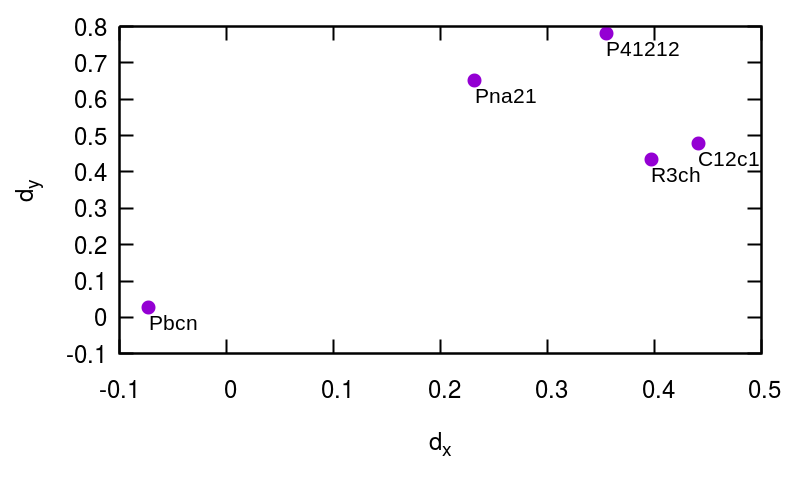 Figure 1
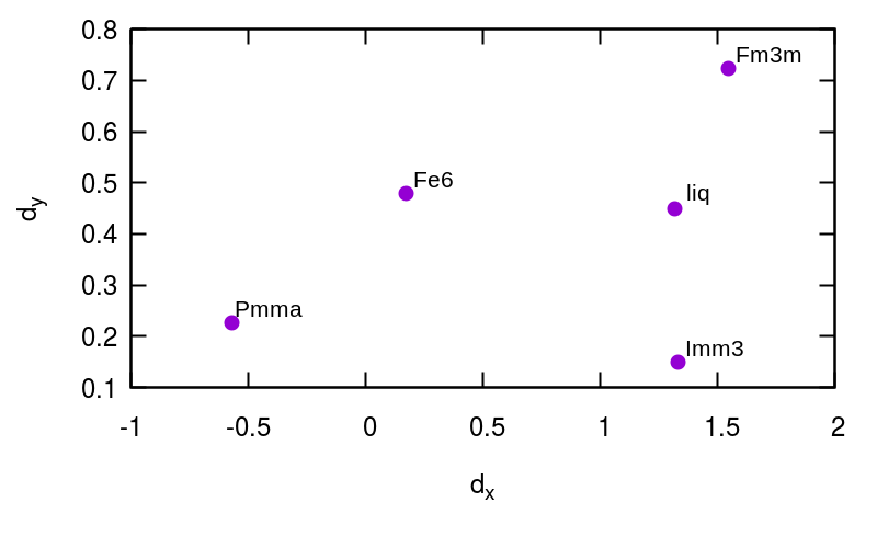 Figure 2
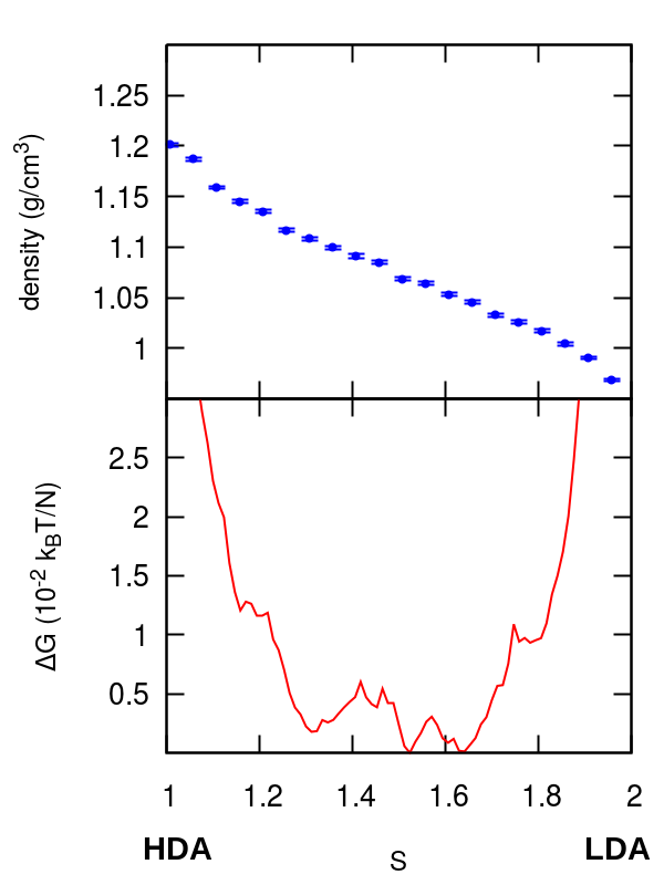 Figure 3
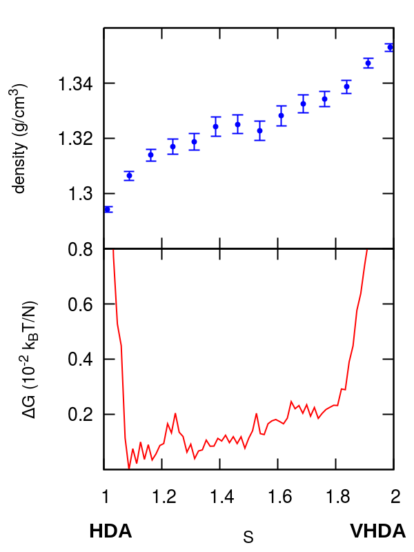 Figure 4
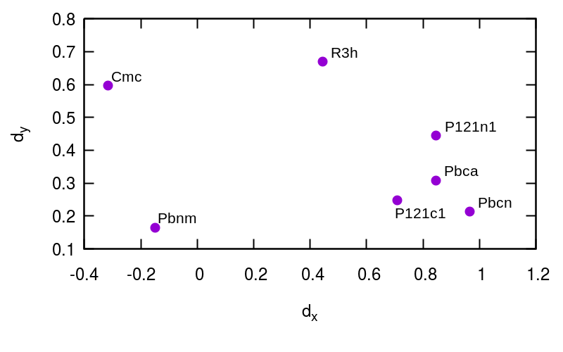 Figure 5
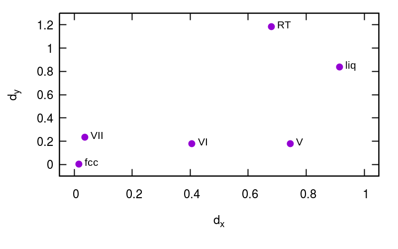 Figure 6
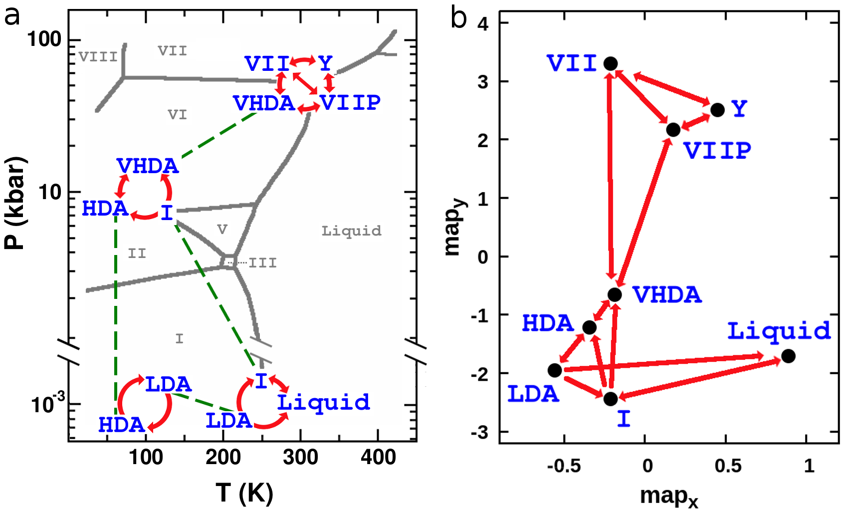 Figure 1
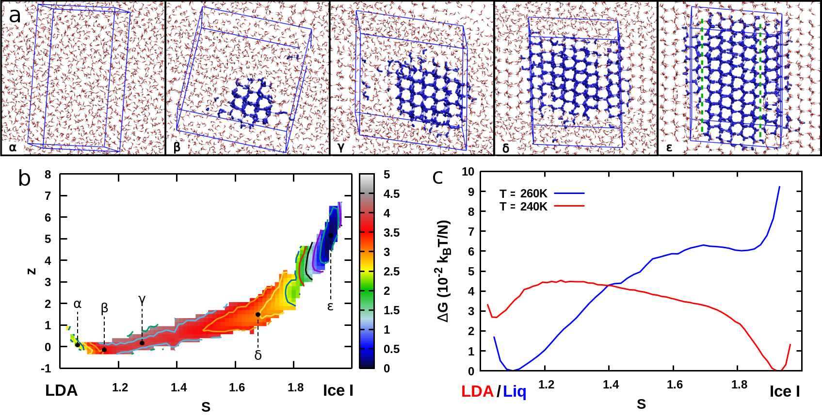 Figure 2
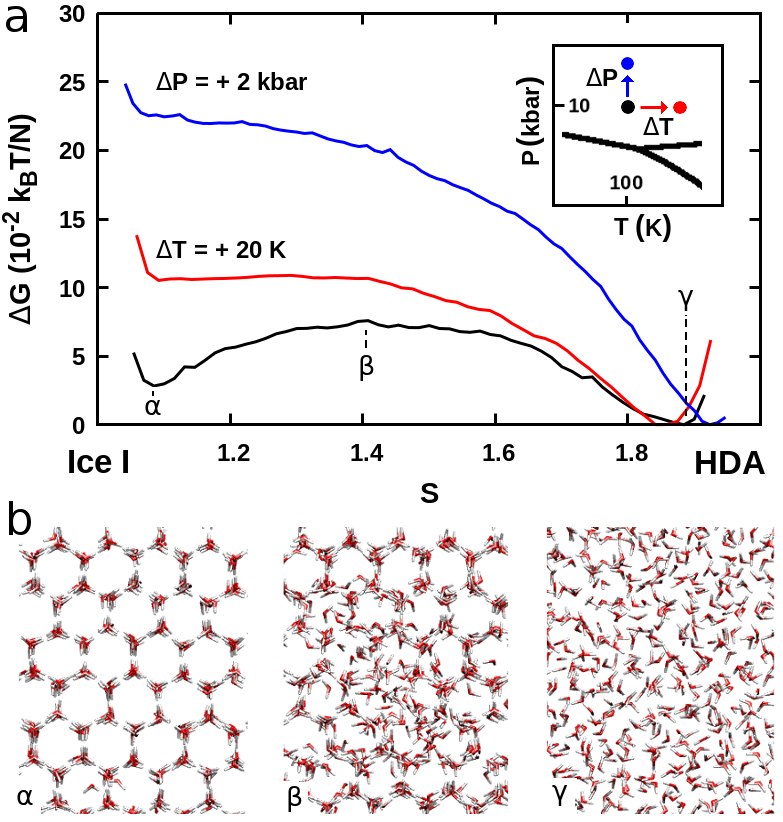 Figure 3
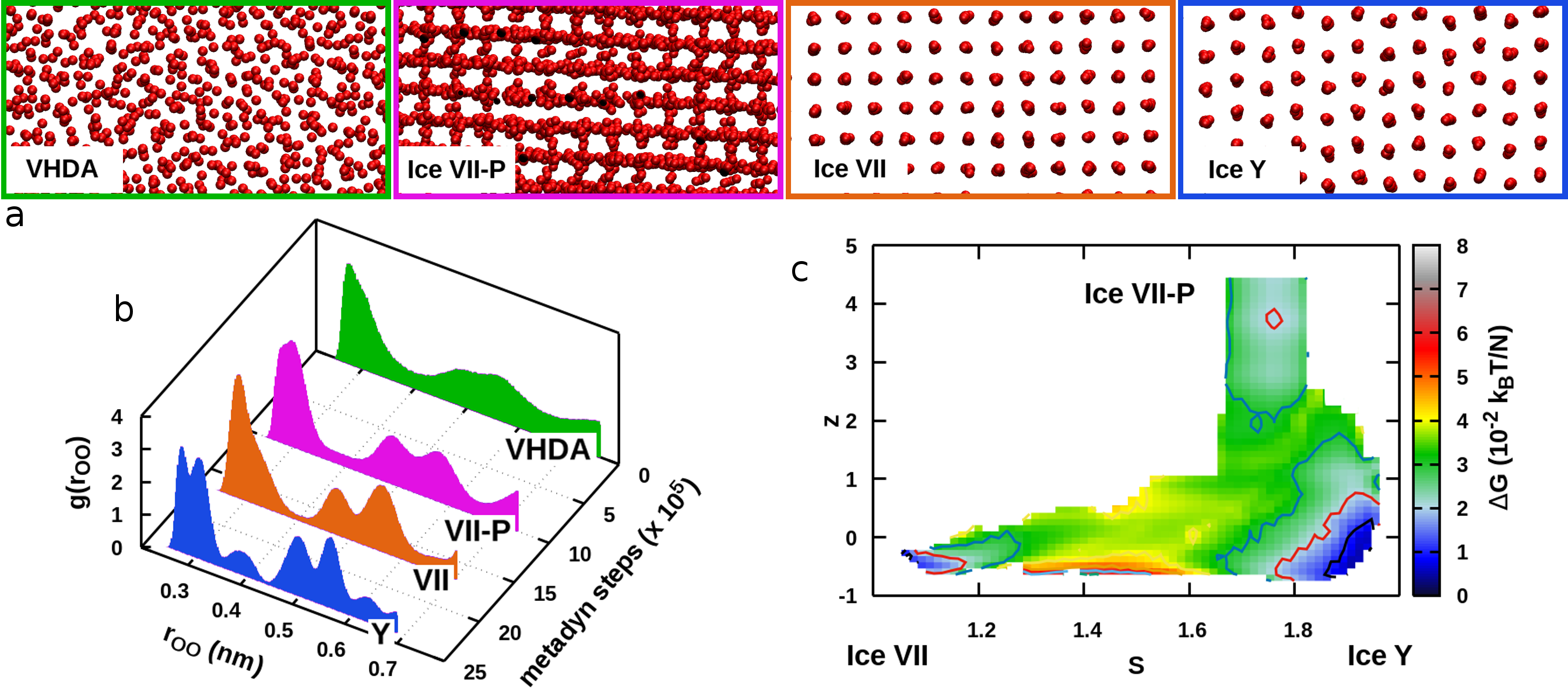 Figure 4
| Å | Å | Å | |||||||||||||||
|---|---|---|---|---|---|---|---|---|---|---|---|---|---|---|---|---|---|
| Fm3m | liq | Imm3 | Fe6 | Pmma | Fm3m | liq | Imm3 | Fe6 | Pmma | Fm3m | liq | Imm3 | Fe6 | Pmma | |||
| Fm3m | - | 0.43 | 0.41 | 1.03 | 1.27 | - | 0.41 | 0.58 | 1.43 | 2.12 | - | 0.53 | 0.74 | 2.10 | 2.93 | ||
| liq | 0.43 | - | 0.29 | 0.84 | 1.11 | 0.41 | - | 0.34 | 1.18 | 1.90 | 0.53 | - | 0.41 | 1.74 | 2.62 | ||
| Imm3 | 0.41 | 0.29 | - | 0.80 | 1.06 | 0.58 | 0.34 | - | 1.18 | 1.92 | 0.74 | 0.41 | - | 1.68 | 2.58 | ||
| Fe6 | 1.03 | 0.84 | 0.80 | - | 0.28 | 1.43 | 1.18 | 1.18 | - | 0.83 | 2.10 | 1.74 | 1.68 | - | 1.15 | ||
| Pmma | 1.27 | 1.11 | 1.06 | 0.28 | - | 2.12 | 1.90 | 1.92 | 0.83 | - | 2.93 | 2.62 | 2.58 | 1.15 | - | ||
| Å | Å | Å | ||||||||||||||||||
|---|---|---|---|---|---|---|---|---|---|---|---|---|---|---|---|---|---|---|---|---|
| fcc | VII | VI | V | RT | liq | fcc | VII | VI | V | RT | liq | fcc | VII | VI | V | RT | liq | |||
| fcc | - | 0.28 | 0.93 | 0.97 | 1.47 | 1.33 | - | 0.40 | 0.68 | 1.09 | 1.86 | 1.63 | - | 0.71 | 0.68 | 1.12 | 2.00 | 1.95 | ||
| VII | 0.28 | - | 0.81 | 0.76 | 1.24 | 1.08 | 0.40 | - | 0.56 | 0.94 | 1.74 | 1.48 | 0.71 | - | 0.62 | 1.04 | 2.13 | 2.01 | ||
| VI | 0.93 | 0.81 | - | 0.63 | 0.98 | 0.90 | 0.68 | 0.56 | - | 0.55 | 1.46 | 1.22 | 0.68 | 0.62 | - | 0.64 | 1.76 | 1.70 | ||
| V | 0.97 | 0.76 | 0.63 | - | 0.87 | 0.66 | 1.09 | 0.94 | 0.55 | - | 1.34 | 1.06 | 1.12 | 1.04 | 0.64 | - | 1.44 | 1.34 | ||
| RT | 1.47 | 1.24 | 0.98 | 0.87 | - | 0.42 | 1.86 | 1.74 | 1.46 | 1.34 | - | 0.66 | 2.00 | 2.13 | 1.76 | 1.44 | - | 0.61 | ||
| liq | 1.33 | 1.08 | 0.90 | 0.66 | 0.42 | - | 1.63 | 1.48 | 1.22 | 1.06 | 0.66 | - | 1.95 | 2.01 | 1.70 | 1.34 | 0.61 | - | ||
| Å | Å | Å | ||||||
|---|---|---|---|---|---|---|---|---|
| hcp | bcc | hcp | bcc | hcp | bcc | |||
| hcp | - | 0.07 | - | 0.29 | - | 0.45 | ||
| bcc | 0.07 | - | 0.29 | - | 0.45 | - | ||
| Å | Å | Å | ||||||||||||
|---|---|---|---|---|---|---|---|---|---|---|---|---|---|---|
| cubic | lonsdaleite | diamond | graphite | cubic | lonsdaleite | diamond | graphite | cubic | lonsdaleite | diamond | graphite | |||
| cubic | - | 2.83 | 2.87 | 3.34 | - | 4.48 | 4.57 | 5.20 | - | 5.54 | 5.63 | 6.40 | ||
| lonsdaleite | 2.83 | - | 0.22 | 0.82 | 4.48 | - | 0.37 | 1.19 | 5.54 | - | 0.38 | 1.22 | ||
| diamond | 2.87 | 0.22 | - | 0.79 | 4.57 | 0.37 | - | 1.13 | 5.63 | 0.38 | - | 1.07 | ||
| graphite | 3.34 | 0.82 | 0.79 | - | 5.20 | 1.19 | 1.13 | - | 6.40 | 1.22 | 1.07 | - | ||
| Å | Å | Å | ||||||||||||
|---|---|---|---|---|---|---|---|---|---|---|---|---|---|---|
| Pm3m | Cmca | Imma | P12c1 | Pm3m | Cmca | Imma | P12c1 | Pm3m | Cmca | Imma | P12c1 | |||
| Pm3m | - | 0.32 | 0.50 | 0.52 | - | 0.42 | 0.53 | 0.73 | - | 0.38 | 0.59 | 0.94 | ||
| Cmca | 0.32 | - | 0.50 | 0.53 | 0.42 | - | 0.53 | 0.73 | 0.38 | - | 0.51 | 0.90 | ||
| Imma | 0.50 | 0.50 | - | 0.11 | 0.53 | 0.53 | - | 0.33 | 0.59 | 0.51 | - | 0.46 | ||
| P12c1 | 0.52 | 0.53 | 0.11 | - | 0.73 | 0.73 | 0.33 | - | 0.94 | 0.90 | 0.46 | - | ||
| Å | Å | Å | |||||||||||||||
|---|---|---|---|---|---|---|---|---|---|---|---|---|---|---|---|---|---|
| S () | S7 (c) | S7 (n) | S12 | S8 | S () | S7 (c) | S7 (n) | S12 | S8 | S () | S7 (c) | S7 (n) | S12 | S8 | |||
| S () | - | 1.20 | 1.21 | 1.23 | 1.25 | - | 1.76 | 1.76 | 1.86 | 1.87 | - | 2.50 | 2.51 | 2.60 | 2.61 | ||
| S7 (c) | 1.20 | - | 0.02 | 0.05 | 0.06 | 1.76 | - | 0.04 | 0.16 | 0.17 | 2.50 | - | 0.06 | 0.19 | 0.19 | ||
| S7 (n) | 1.21 | 0.02 | - | 0.06 | 0.06 | 1.76 | 0.04 | - | 0.17 | 0.16 | 2.51 | 0.06 | - | 0.19 | 0.19 | ||
| S12 | 1.23 | 0.05 | 0.06 | - | 0.03 | 1.86 | 0.16 | 0.17 | - | 0.08 | 2.60 | 0.19 | 0.19 | - | 0.10 | ||
| S8 | 1.25 | 0.06 | 0.06 | 0.03 | - | 1.87 | 0.17 | 0.16 | 0.08 | - | 2.61 | 0.19 | 0.19 | 0.10 | - | ||
| Å | Å | Å | |||||||||
|---|---|---|---|---|---|---|---|---|---|---|---|
| M-3C | M-P6 | M-6H | M-3C | M-P6 | M-6H | M-3C | M-P6 | M-6H | |||
| M-3C | - | 0.10 | 0.22 | - | 0.35 | 0.68 | - | 0.57 | 0.92 | ||
| M-P6 | 0.10 | - | 0.21 | 0.35 | - | 0.64 | 0.57 | - | 1.05 | ||
| M-6H | 0.22 | 0.21 | - | 0.68 | 0.64 | - | 0.92 | 1.05 | - | ||
| Å | Å | Å | |||||||||||||||
|---|---|---|---|---|---|---|---|---|---|---|---|---|---|---|---|---|---|
| Coes. | Crist. | Quartz | Stishov. | Tridym. | Coes. | Crist. | Quartz | Stishov. | Tridym. | Coes. | Crist. | Quartz | Stishov. | Tridym. | |||
| Stishov. | - | 0.77 | 0.82 | 1.03 | 0.91 | - | 1.03 | 1.09 | 1.41 | 1.49 | - | 1.61 | 1.42 | 1.87 | 2.04 | ||
| Coes. | 0.77 | - | 0.09 | 0.64 | 0.24 | 1.03 | - | 0.25 | 0.57 | 0.61 | 1.61 | - | 0.41 | 0.57 | 0.71 | ||
| Quartz | 0.82 | 0.09 | - | 0.63 | 0.19 | 1.09 | 0.25 | - | 0.50 | 0.51 | 1.42 | 0.41 | - | 0.63 | 0.77 | ||
| Tridym. | 1.03 | 0.64 | 0.63 | - | 0.59 | 1.41 | 0.57 | 0.50 | - | 0.35 | 1.87 | 0.57 | 0.63 | - | 0.31 | ||
| Crist. | 0.91 | 0.24 | 0.19 | 0.59 | - | 1.49 | 0.61 | 0.51 | 0.35 | - | 2.04 | 0.71 | 0.77 | 0.31 | - | ||
| Å | Å | Å | ||||||
|---|---|---|---|---|---|---|---|---|
| Fm3m | Pm3m | Fm3m | Pm3m | Fm3m | Pm3m | |||
| Fm3m | - | 0.23 | - | 0.84 | - | 1.19 | ||
| Pm3m | 0.23 | - | 0.84 | - | 1.19 | - | ||
| Å | Å | Å | |||||||||||||||
|---|---|---|---|---|---|---|---|---|---|---|---|---|---|---|---|---|---|
| Pbcn | R3ch | C12c1 | Pna21 | P41212 | Pbcn | R3ch | C12c1 | Pna21 | P41212 | Pbcn | R3ch | C12c1 | Pna21 | P41212 | |||
| Pbcn | - | 0.39 | 0.41 | 0.53 | 0.58 | - | 0.63 | 0.68 | 0.73 | 0.82 | - | 1.05 | 1.20 | 1.10 | 1.37 | ||
| R3ch | 0.39 | - | 0.04 | 0.29 | 0.35 | 0.63 | - | 0.07 | 0.27 | 0.35 | 1.05 | - | 0.20 | 0.27 | 0.44 | ||
| C12c1 | 0.41 | 0.04 | - | 0.27 | 0.33 | 0.68 | 0.07 | - | 0.26 | 0.32 | 1.20 | 0.20 | - | 0.31 | 0.36 | ||
| Pna21 | 0.53 | 0.29 | 0.27 | - | 0.15 | 0.73 | 0.27 | 0.26 | - | 0.21 | 1.10 | 0.27 | 0.31 | - | 0.36 | ||
| P41212 | 0.58 | 0.35 | 0.33 | 0.15 | - | 0.82 | 0.35 | 0.32 | 0.21 | - | 1.37 | 0.44 | 0.36 | 0.36 | - | ||
| Å | Å | |||||||||||||||
|---|---|---|---|---|---|---|---|---|---|---|---|---|---|---|---|---|
| Cmcm | Pbnm | R3h | P121c1 | Pbca | P121n1 | Pbcn | Cmcm | Pbnm | R3h | P121c1 | Pbca | P121n1 | Pbcn | |||
| Cmcm | - | 0.32 | 0.60 | 0.87 | 0.91 | 0.89 | 0.97 | - | 0.49 | 0.84 | 1.09 | 1.18 | 1.15 | 1.28 | ||
| Pbnm | 0.32 | - | 0.50 | 0.76 | 0.79 | 0.77 | 0.85 | 0.49 | - | 0.75 | 0.94 | 1.01 | 0.99 | 1.12 | ||
| R3h | 0.60 | 0.50 | - | 0.50 | 0.52 | 0.53 | 0.57 | 0.84 | 0.75 | - | 0.49 | 0.55 | 0.54 | 0.66 | ||
| P121c1 | 0.87 | 0.76 | 0.50 | - | 0.13 | 0.21 | 0.18 | 1.09 | 0.94 | 0.49 | - | 0.20 | 0.24 | 0.29 | ||
| Pbca | 0.91 | 0.79 | 0.52 | 0.13 | - | 0.14 | 0.16 | 1.18 | 1.01 | 0.55 | 0.20 | - | 0.19 | 0.21 | ||
| P121n1 | 0.89 | 0.77 | 0.53 | 0.21 | 0.14 | - | 0.20 | 1.15 | 0.99 | 0.54 | 0.24 | 0.19 | - | 0.26 | ||
| Pbcn | 0.97 | 0.85 | 0.57 | 0.18 | 0.16 | 0.20 | - | 1.28 | 1.12 | 0.66 | 0.29 | 0.21 | 0.26 | - | ||
| Å | ||||||||||||||||
| Cmcm | Pbnm | R3h | P121c1 | Pbca | P121n1 | Pbcn | ||||||||||
| Cmcm | - | 0.56 | 1.18 | 1.50 | 1.64 | 1.59 | 1.71 | |||||||||
| Pbnm | 0.56 | - | 1.05 | 1.33 | 1.45 | 1.42 | 1.54 | |||||||||
| R3h | 1.18 | 1.05 | - | 0.54 | 0.64 | 0.61 | 0.72 | |||||||||
| P121c1 | 1.50 | 1.33 | 0.54 | - | 0.24 | 0.23 | 0.29 | |||||||||
| Pbca | 1.64 | 1.45 | 0.64 | 0.24 | - | 0.22 | 0.23 | |||||||||
| P121n1 | 1.59 | 1.42 | 0.61 | 0.23 | 0.22 | - | 0.24 | |||||||||
| Pbcn | 1.71 | 1.54 | 0.72 | 0.29 | 0.23 | 0.24 | - | |||||||||
| Å | Å | Å | ||||||
|---|---|---|---|---|---|---|---|---|
| Pbca | P121c1 | Pbca | P121c1 | Pbca | P121c1 | |||
| Pbca | - | 0.09 | - | 0.17 | - | 0.21 | ||
| P121c1 | 0.09 | - | 0.17 | - | 0.21 | - | ||
| Å | Å | Å | ||||||
|---|---|---|---|---|---|---|---|---|
| Pbca | P121n1 | Pbca | P121n1 | Pbca | P121n1 | |||
| Pbca | - | 0.09 | - | 0.23 | - | 0.42 | ||
| P121c1 | 0.09 | - | 0.23 | - | 0.42 | - | ||
| Density (kg/m3) | Diffusion Coeff. ( cm2/s) | |
|---|---|---|
| LDA 100 K | 987 1 | 0.000041 0.000008 |
| LDA 240 K | 980.9 0.3 | 0.29 0.03 |
| liq 260 K | 985.2 0.1 | 0.8407 0.0009 |
| liq 300 K | 976.3 0.1 | 2.619 0.008 |
Peer Reviews
No public reviews on file for this paper yet. If you reviewed it on a platform where reviews are public (OpenReview, ICLR, NeurIPS, ICML), you can paste yours below so the community can read it here.
Videos
No videos yet. Explain this paper in a talk, walkthrough, or lecture? Add one.
Navigating at Will on the Water Phase Diagram
S. Pipolo
Present affiliation: Univ. Lille, CNRS, Centrale Lille, ENSCL, Univ. Artois, UMR 8181 - UCCS - Unité de Catalyse et Chimie du Solide, F-59000 Lille, France
Sorbonne Universités, UPMC Univ. Paris 06, CNRS UMR 7590, IRD UMR 206, MNHN, IMPMC, F-75005 Paris, France
M. Salanne
Sorbonne Universités, UPMC Univ. Paris 06, CNRS, Laboratoire PHENIX, F-75005 Paris, France
G. Ferlat
S. Klotz
A.M. Saitta
F. Pietrucci
Sorbonne Universités, UPMC Univ. Paris 06, CNRS UMR 7590, IRD UMR 206, MNHN, IMPMC, F-75005 Paris, France
Present affiliation: Univ. Lille, CNRS, Centrale Lille, ENSCL, Univ. Artois, UMR 8181 - UCCS - Unité de Catalyse et Chimie du Solide, F-59000 Lille, France
Sorbonne Universités, UPMC Univ. Paris 06, CNRS UMR 7590, IRD UMR 206, MNHN, IMPMC, F-75005 Paris, France
Sorbonne Universités, UPMC Univ. Paris 06, CNRS, Laboratoire PHENIX, F-75005 Paris, France
Sorbonne Universités, UPMC Univ. Paris 06, CNRS UMR 7590, IRD UMR 206, MNHN, IMPMC, F-75005 Paris, France
Now at: Unité de Catalyse et Chimie du Solide, Université de Lille 1, 59655 Villeneuve d’Ascq, France
Sorbonne Universités, UPMC Univ. Paris 06, CNRS UMR 7590, IRD UMR 206, MNHN, IMPMC, F-75005 Paris, France
Sorbonne Universités, UPMC Univ. Paris 06, CNRS, Laboratoire PHENIX, F-75005 Paris, France
Sorbonne Universités, UPMC Univ. Paris 06, CNRS UMR 7590, IRD UMR 206, MNHN, IMPMC, F-75005 Paris, France
Abstract
Despite the simplicity of its molecular unit, water is a challenging system because of its uniquely rich polymorphism and predicted but yet unconfirmed features. Introducing a novel space of generalized coordinates that capture changes in the topology of the interatomic network, we are able to systematically track transitions among liquid, amorphous and crystalline forms throughout the whole phase diagram of water, including the nucleation of crystals above and below the melting point. Our approach, based on molecular dynamics and enhanced sampling / free energy calculation techniques, is not specific to water and could be applied to very different structural phase transitions, paving the way towards the prediction of kinetic routes connecting polymorphic structures in a range of materials.
Computational structure prediction methods Pickard and Needs (2011); Glass et al. (2006) have strongly contributed to the rapid increase of new predicted phases of materials with enhanced properties for applications (see, e.g., Ref. Wilmer et al. (2012)). However, at present, no general approach has been developed for guiding experiments through the pathways connecting stable structures of condensed matter. Moreover, metastable phases are very often involved in phase transitions Schreiber et al. (2016) and sometimes their kinetic stability is very high Himoto et al. (2014). Thus, in order to recover the global minimum structure, one needs to find specific routes, by e.g. acting on pressure or temperature, in a way that is not at all trivial to guess Radha et al. (2015). A precise understanding of transition mechanisms and the corresponding kinetics is therefore the key to explain and control the behavior of matter. The case of water is emblematic because several experiments have disclosed connections between stable and metastable phases Bartels-Rausch et al. (2012); Palmer et al. (2014); Mishima and Stanley (1998); Klotz et al. (2005) and recently simulations have highlighted the importance of metastable states in understanding the mechanism of phase transitions and related transformations Russo et al. (2014). A classic example is the connection between the crystalline ice stable at ambient pressure (Ice I), and the low-density amorphous (LDA) and high-density amorphous (HDA) ices: by compressing Ice I up to 10 kbar at 80 K one obtains HDA instead of Ice VI,Mishima et al. (1984) which may be transformed into LDA by decompression of HDA at 130 K Klotz et al. (2005) or by heating recovered HDA at ambient pressure to beyond 130 K; Mishima and Stanley (1998) finally Ice I is recovered by heating up LDA. Similar connections between crystalline and amorphous ices are found in the high-pressure region of the water phase diagram where a very-high-density amorphous (VHDA) ice, plastic ices and crystalline structures with complex hydrogen-bond network (e.g. Ice VII) have been observed or predicted. Amann-Winkel et al. (2016); Himoto et al. (2014)
Molecular dynamics (MD), a simulation method that yields the atomic trajectories as a function of time at given thermodynamic conditions, is in principle able to track such transitions. The kinetic barriers are however generally too large to allow an efficient exploration of the configuration space within typical MD timescales. Hence, so far it has been necessary to introduce (i) simplistic interaction models Moore and Molinero (2011) and/or (ii) seeding techniques Espinosa et al. (2016). Another approach consists in using enhanced sampling techniques that accelerate the occurrence of rare events by focusing on low-dimensional order parameters, also called collective variables (CV) Pietrucci (2017). Yet the CVs available to describe phase transitions are specifically designed for a given type of structural transformation Lechner and Dellago (2008); Martoňák et al. (2003); Haji-Akbari and Debenedetti (2015), while no general CV scheme has been proven successful for a wide class of problems, in particular those involving amorphous systems. Recently, distance metrics developed for condensed matter Valle and Oganov (2010); Gallet and Pietrucci (2013); Pietrucci and Martoák (2015); Pietrucci and Saitta (2015); Zhu et al. (2016); De et al. (2016) have been proven to be successful in classifying structures in molecular or extended systems based on their atomic environment and/or interatomic network. Here we show that by combining enhanced sampling techniques with a novel CV based on a general metric we are able to define in an efficient way the topological space of transformations among liquid, amorphous, and crystalline forms of water. This allows exploring at will the phase diagram along pathways connecting minimum-energy structures with a single, general approach, capable to characterize mechanisms and energetics.
Our CV scheme relies on the concept of generalized distances between configurations of the system, as defined from relative atomic positions, and it only requires to postulate the initial and final states of the target transformation, without any assumption on the pathway. The transformation is represented in a two-dimensional space of path CVs Branduardi et al. (2007), with quantifying the progress of the transformation and allowing to discriminate between different pathways and to represent transitions to states that are not the target ones. In such a CV scheme each configuration of the system is associated with a permutation invariant vector Gallet and Pietrucci (2013) (PIV), built-up from inter-atomic Cartesian distances. The PIV is built starting from atom-type-specific ordered blocks, , with elements
[TABLE]
Here is the position vector of the -th atom of type (oxygen or hydrogen), with , ; are coefficients that define the PIV variant (they are all equal to one in the original formulation); and are the volume of the simulation box and a reference volume (details below) respectively; is a switching function monotonically decreasing from one to zero as increases (see Ref. sup for more details). In order to define the PIV, first the elements of each block are sorted in ascending ordered, then the different blocks are simply joined together resulting in a PIV of components, that we indicate with . The sorting operation within each block introduces invariance upon permutation of identical atoms. The volume scaling factor (absent in Ref. Gallet and Pietrucci (2013)) was found to be important to avoid violent fluctuations of the cell parameters during metadynamics.
Distances between generic configurations X and Y are computed as squared Euclidean distances between the corresponding PIVs (), and used to map each configuration of the system (X) into a point in the 2D space defined by the path CVs Branduardi et al. (2007), built starting from only two reference configurations A and B representing the initial and final state of the transformation:
[TABLE]
The two coordinates track the progress from A to B and the distance from A and B, respectively. We remark that this formulation does not contain any guess about the mechanism of the transformation, and that the freedom granted by the coordinate allows to explore also the formation of unexpected metastable structures different from A and B (e.g., Ice VII-P in Figure 4-c). There is some freedom in the choice of the parameter : in this work we adopted , conveniently localizing the free energy basins of reference states A and B around and , respectively, and leading to smooth transformation pathways and landscapes. A much larger would produce very irregular and discontinuous pathways, while a much smaller one would hamper the resolution of different phases. We used metadynamics Laio and Parrinello (2002) for the discovery of continuum pathways between locally stable configurations, and umbrella sampling Torrie and Valleau (1977) for the reconstruction of precise free energy landscapes. Computational details are given in Ref. sup .
In Figure 1-a we draw the pathways we followed on the phase diagram of a realistic model of water Abascal and Vega (2005), navigating within and across free-energy basins using standard MD and enhanced sampling techniques, respectively. Figure 1-b shows a two-dimensional map (see also Ref. Pietrucci and Martoák (2015)) of distances between the visited crystalline and amorphous structures: the metric employed to define the CVs is able to scatter the different phases in a way that recalls the topology of the phase diagram, representing kinetically connected phases as neighbors, and kinetically disconnected ones as far apart.
As a starting point we analyze the crystallization of Ice I both from the liquid and the LDA phases at bar and over a range of temperatures around the melting point ( K for the adopted interatomic potential Abascal and Vega (2005)). The initial configurations have been respectively obtained by cooling down an equilibrium liquid phase from K and heating up a LDA structure from K sup . Both crystallization transitions have been achieved multiple times in metadynamics simulations at K and K and they are all characterized by (i) a nucleation mechanism that we show in Figure 2 for the LDA–Ice I transformation at K, (ii) the formation of a crystal nucleus of cubic symmetry (Ice Ic), and (iii) a final state with either a perfect cubic symmetry or made up of layers of cubic Ic and hexagonal Ih ice (see last snapshot in Figure 2-a). This last feature is in agreement with experimental findings Malkin et al. (2012), and our results show that the formation of stacking disordered Ice I may also proceed via the merging of Ic-nuclei as well as via (i) random growth of Ic and Ih layers Malkin et al. (2015) and (ii) direct formation of Ic-Ih nuclei Haji-Akbari and Debenedetti (2015). In Figure 2-b we display the free energy profiles for the liquid–Ice I and LDA–Ice I transformations, respectively above and below the melting point. The calculated relative stabilities of the various phases agree with the phase diagram of the water model, and the order of magnitude of the free-energy profiles is consistent with free-energy differences calculated in previous works Vega et al. (2008). We remark that crystallizing the liquid above the melting temperature, in the bulk, without any seeds and with a very realistic water model, shows that our approach allows to perform very challenging transformations even in unfavorable conditions, reaching metastable states (here Ice I) starting from the global minimum.
In order to carry on our continuous journey towards high pressure, we follow the experimental routes by cooling down Ice I to K, and then compressing it at kbar using standard MD: in the neighborhood of this point of the phase diagram we explore (with enhanced sampling simulations) the transformation to HDA as a function of temperature and pressure. We find that the free-energy barrier decreases when temperature and pressure increase, as we show in Figure 3. Furthermore we note that although the free energy of Ice I is higher than the one of HDA already at kbar and K (which is expected since Ice I is not the stable phase in this region of the phase diagram), the free-energy barrier is nonzero. This result is in accordance with a common interpretation of the Ice I–HDA transformation Mishima and Stanley (1998); Chen and Yoo (2011) that can be seen as an extrapolation to low temperatures and high pressures of the Ice I–Liquid coexistence line. Even if this description is mostly qualitative, it certainly invigorates the idea that low-density crystalline ice is unstable with respect to denser disordered forms at high pressures, and that such instability occurs at higher pressures as temperature is decreased.
The HDA phase we obtain is then (i) decompressed at ambient pressure and transformed into LDA to close the loop of transitions at low pressure, (ii) compressed at kbar and transformed into VHDA. Free-energy and density profiles for HDA-LDA and HDA-VHDA transformations are provided sup . The HDA-VHDA transformation connects the low-pressure and high-pressure regions that we explore in this work. The VHDA phase is compressed and heated until it reaches kbar and K, and at this point we address its crystallization to Ice VII. While simulating the VHDA–Ice VII transformation via metadynamics we observe that the system visits two additional metastable configurations. This result demonstrates that our method does not constrain the system to sample configurations along a simple path connecting the two reference structures, but rather allows it to follow complex mechanisms and discover new free energy basins. The metastable structures differ markedly from the other phases, as shown in Figure 4 where we compare representative snapshots and the oxygen-oxygen radial distribution functions. The first metastable phase is identified as the plastic Ice VII-P, which had already been proposed by Himoto et al. Himoto et al. (2014). Oxygen atoms are arranged in a rather ordered crystalline network, whereas the hydrogen bond network changes dynamically: the correlation decay time of molecular dipoles is more than one order of magnitude shorter than that of Ice VII at the same thermodynamic conditions. The second metastable phase (labeled here “Ice Y”) is characterized by a tetragonal oxygen lattice and stacked layers of hydrogen-bond networks. We leave a detailed investigation of this phase for future works (the atomic coordinates are provided sup ). The flexibility of our method in representing transformations among several states in a two-dimensional CV space is illustrated in the free energy landscape connecting the three crystalline phases (Ice VII, Ice VII-P and Ice Y) shown on Figure 4-c.
In conclusion, we propose a versatile method allowing the efficient simulation of phase transitions in condensed matter. We illustrated the approach by tackling the difficult problem of poly(a)morphism in water, including kinetically challenging amorphous-to-crystalline and liquid-to-crystalline transitions. In particular, we simulated transformations between the LDA, HDA, liquid and Ice I phases in the low-pressure region of the phase diagram and among VHDA and Ice VII in the high-pressure region. In both cases, important mechanistic informations could be extracted from the simulations, highlighting the role of metastable structures during phase transitions. Thanks to a very general formulation, the proposed approach is not restricted to specific transitions of a single material. Analysis of 50 experimental polymorphs belonging to 13 different materials (covalent, metallic, ionic, and molecular) indicates that the PIV-based metric is able to resolve all physically-distinct structures sup , suggesting a broad applicability of our simulation approach. The ability to discover transformation mechanisms, simulate nucleation events, and reconstruct free energy landscapes and kinetic barriers – all in a robust and systematic way – is highly complementary to structure prediction and materials discovery efforts.
Acknowledgements.
FP thanks Grégoire A. Gallet for help with the implementation of a preliminary version of the PIV path collective variables. This work was funded within the Investissements d’Avenir program under reference ANR-11-IDEX-0004-02, within the framework of the cluster of excellence MATériaux Interfaces Surfaces Environnement (MATISSE) led by Sorbonne Universités. We acknowledge calculations performed on the Gnome cluster at UPMC, on the Occigen cluster at CINES, Montpellier, France, and on the Ada cluster at IDRIS, Orsay, France, under GENCI allocations 2015-091387 and 2016-091387.
Computational details
In all enhanced sampling simulations the PIV is defined employing the following switching function of interatomic distances :
[TABLE]
The decay range of the switching function is defined in order to maximize the distance between the two target phases using the initial volume of the box for each simulation as the reference volume . The set of parameters for eq. (4) used in simulations of Figures 2, 3 and 4 are respectively , and ( values are in nm). The first set of parameters is also used for the illustrative map in Figure 1-b, that is constructed, starting from random 2D positions of the representative points, by minimizing the difference between PIV distances and map distances with a Monte Carlo procedure, until obtaining errors smaller than 6%. and (eq.(1)) are used to construct the PIVs for the crystallization of Ice I, in all other transformations since oxygen-oxygen terms are sufficient to represent the transformation pathways.
The potential used to model interactions between water molecules is TIP4P/2005 Abascal and Vega (2005), with periodically-repeated boxes of molecules (except for the 2D umbrella sampling in Figure 4 where ). MD and enhanced sampling simulations were performed in the ensemble. Time constants for pressure Berendsen et al. (1984) and temperature Bussi et al. (2007) coupling of ps and ps were respectively used. Due to the sizable computational cost of PIV construction, enhanced sampling simulations are on average 10 (50) times slower than standard MD for a PIV built-up with oxygen (oxygen and hydrogen) atoms.
Metadynamics simulations, of typical duration between and ns, allowed to overcome kinetic barriers and quickly explore many different transformations, discovering mechanisms as well as unexpected ice phases. For instance, we could repeatedly simulate the crystallization of liquid water or of LDA water at different conditions above and below the melting point. Typical width, height, and deposition stride of the repulsive Gaussians are , , kJ/mol, ps. To obtain free energy landscapes of high statistical precision we exploited umbrella sampling simulations, seeded from the structures explored with metadynamics. Each umbrella sampling window has a typical duration of ns, with the last ns (corresponding typically to more than 1000 times the autocorrelation decay time of the variables) employed to reconstruct the free energy landscape using the weighted histogram analysis method Roux (1995). In the landscapes of Figures 2 and 4 we restricted the sampling to the relevant regions of the landscape, i.e., those containing the transition pathways. Statistical errors on free energies, estimated by bootstrapping or by cutting each trajectory in 5 segments and taking standard deviations, are smaller than . Periodic boundary conditions are applied and the 3D particle-mesh-Ewald approach is used for electrostatics with a real-space cutoff of nm (the same cutoff is used for van der Waals interactions). GROMACS 5.1.2 Berendsen et al. (1995) and a modified version of the PLUMED 2 plugin Tribello et al. (2014) (soon available from www.plumed.org or upon request) were employed to perform MD and enhanced sampling simulations.
PIV distances between polymorphs of different types of materials
In this section we analyze PIV distances in a set of 50 experimental polymorphs of ionic, molecular, metallic, and covalent solids, including elements, binary, ternary and organic compounds. The aim is to test whether our methodology – based on a general formulation that is not designed specifically for water – might be applied to several different classes of materials. All crystal structures are taken from the Crystallography Open Database (www.crystallography.net). In Tables 1-13 we report PIV distances between polymorphs of iron, silicon, sodium, carbon, phosphorus, sulphur, SiC, SiO2, RbCl, Fe2O3, MgSiO3, benzene, and paracetamol. In all cases, to avoid system-dependent fine tuning, we included all atoms in the PIV definition and we tested the same set of three different switching functions of interatomic distances, with , and 2.5, 3.5, or 4.5 Å, respectively. In the tables, PIV distances are scaled by the square root of the number of atoms, according to the definition in Ref. Pietrucci and Martoák (2015), to facilitate their comparison across different materials. Polymorphs are presented in order of decreasing density. To provide a reference allowing to appreciate the good separation between different polymorphs, we performed 100 ps-long MD simulations at 300 K of a single polymorph of iron (2000 atoms, embedded atoms potential Mendelev et al. (2003)), silicon (2304 atoms, Stillinger-Weber potential Stillinger and Weber (1985)), and benzene (108 molecules, OPLS-AA potential Jorgensen et al. (1996)), finding a maximum value of PIV distance between snapshots of each system (i.e., a thermal spread) equal to 0.016, 0.004, and 0.005, respectively (with Å). With similar MD simulations we obtained reference structures for liquid iron and silicon, at 2500 K, also reported in Tables 1 and 2 for comparison.
It has been pointed out that, from a mathematical point of view, sets of points can be artificially built displaying a same set of sorted distances Bartók et al. (2013). Nevertheless, as shown in this work as well as in Ref. Pietrucci and Martoák (2015), the PIV-based metric is able to resolve, in all the crystallographic cases considered so far, the structures corresponding to physically-distinct forms of a material (e.g., different polymorphs or different amorphous forms), whereas it does not separate the structures corresponding to physically-equivalent realizations of a same form (e.g., independent configurations belonging to a liquid, or to a same amorphous form). Not only the former, but also the latter is a very convenient feature of the present approach, leading to a compact and well-defined free energy basin even for liquid phases and amorphous forms. In the same spirit, invariance under permutation of identical atoms conveniently overlaps physically-equivalent structures differing only by the labelling of atoms.
In figure S1 we show 2D maps of PIV distances Pietrucci and Martoák (2015), generated using values in Tables 1, 2, 10, and 11 with Å. Note that the points size is larger than the maximum value of intra-polymorph PIV distances reported above.
Amorphous–amorphous transformations
In this section we present an analysis of the HDA-LDA and HDA–VHDA transformations. In Figure S2 we report density and free energy profiles along the pathways of the two transformations obtained from umbrella sampling simulations. Density changes smoothly with the progress of the transformation, the profiles show several local minima but free energy barriers are typically smaller than the ones of the transformations reported in the manuscript, especially for the HDA-VHDA transformation, where they are of the order of magnitude of the estimated errors (see Methods section). This is in agreement with previous computational studies on the compression of the HDA form Chiu et al. (2013), where no hysteresis behavior is observed during compression/decompression cycles. The set of parameters used to define the switching function for the HDA–LDA and HDA–VHDA simulations of Figure S2 are respectively and . For more computational details see the Methods section.
Comparison of LDA and liquid: densities and diffusion coefficients
We report in Table 14 the densities and the diffusion coefficients obtained from four 10 ns-long MD simulations at P = 1 bar, of (i) LDA at T = 100 K (ii), LDA heated up at T = 240 K (iii), the liquid phase cooled down at T = 260 K, and (iv) the liquid phase at T = 300 K.
References
- Abascal and Vega (2005)
J. L. Abascal and C. Vega, J. Chem. Phys. 123, 234505 (2005).
- Berendsen et al. (1984)
H. J. Berendsen, J. v. Postma, W. F. van Gunsteren, A. DiNola, and J. Haak, J. Chem. Phys. 81, 3684 (1984).
- Bussi et al. (2007)
G. Bussi, D. Donadio, and M. Parrinello, J. Chem. Phys. 126, 014101 (2007).
- Roux (1995)
B. Roux, Comput. Phys. Commun. 91, 275 (1995).
- Berendsen et al. (1995)
H. J. Berendsen, D. van der Spoel, and R. van Drunen, Comput. Phys. Commun. 91, 43 (1995).
- Tribello et al. (2014)
G. A. Tribello, M. Bonomi, D. Branduardi, C. Camilloni, and G. Bussi, Comput. Phys. Commun. 185, 604 (2014).
- Pietrucci and Martoák (2015)
F. Pietrucci and R. Martoák, J. Chem. Phys. 142, 104704 (2015).
- Mendelev et al. (2003)
M. Mendelev, S. Han, D. Srolovitz, G. Ackland, D. Sun, and M. Asta, Philosoph. Mag. 83, 3977 (2003).
- Stillinger and Weber (1985)
F. H. Stillinger and T. A. Weber, Phys. Rev. B 31, 5262 (1985).
- Jorgensen et al. (1996)
W. L. Jorgensen, D. S. Maxwell, and J. Tirado-Rives, J. Am. Chem. Soc 118, 11225 (1996).
- Bartók et al. (2013)
A. P. Bartók, R. Kondor, and G. Csányi, Phys. Rev. B 87, 184115 (2013).
- Chiu et al. (2013)
J. Chiu, F. W. Starr, and N. Giovambattista, J. Chem. Phys. 139, 184504 (2013).
The reference list from the paper itself. Each links out to its DOI / PubMed record.
- 1Pickard and Needs (2011) C. J. Pickard and R. Needs, J. Phys. Condens. Matter 23 , 053201 (2011).
- 2Glass et al. (2006) C. W. Glass, A. R. Oganov, and N. Hansen, Comput. Phys. Commun. 175 , 713 (2006).
- 3Wilmer et al. (2012) C. E. Wilmer, M. Leaf, C. Y. Lee, O. K. Farha, B. G. Hauser, J. T. Hupp, and R. Q. Snurr, Nat. Chem. 4 , 83 (2012).
- 4Schreiber et al. (2016) R. E. Schreiber, L. Houben, S. G. Wolf, G. Leitus, Z.-L. Lang, J. J. Carbó, J. M. Poblet, and R. Neumann, Nat. Chem. 9 , 369 (2016).
- 5Himoto et al. (2014) K. Himoto, M. Matsumoto, and H. Tanaka, Phys. Chem. Chem. Phys. 16 , 5081 (2014).
- 6Radha et al. (2015) A. V. Radha, L. Lander, G. Rousse, J. M. Tarascon, and A. Navrotsky, J. Mater. Chem. A 3 , 2601 (2015).
- 7Bartels-Rausch et al. (2012) T. Bartels-Rausch, V. Bergeron, J. H. Cartwright, R. Escribano, J. L. Finney, H. Grothe, P. J. Gutiérrez, J. Haapala, W. F. Kuhs, J. B. Pettersson, et al., Rev. Mod. Phys. 84 , 885 (2012).
- 8Palmer et al. (2014) J. C. Palmer, F. Martelli, Y. Liu, R. Car, A. Z. Panagiotopoulos, and P. G. Debenedetti, Nature 510 , 385 (2014).