Time-dependent density-functional theory for strongly interacting electrons
Luis Cort, Daniel Karlsson, Giovanna Lani, Robert van Leeuwen

TL;DR
This paper analytically investigates the exact exchange-correlation kernel in time-dependent density functional theory for strongly interacting electrons, revealing the dominant instantaneous terms and the conditions under which the adiabatic approximation fails.
Contribution
It provides an analytical expansion of the exchange-correlation kernel in the strong interaction limit and compares it with the strictly correlated electron approach, highlighting the approximation's validity.
Findings
Leading terms in the kernel act instantaneously in the strong interaction limit.
Memory effects appear only in higher-order terms of the expansion.
The adiabatic strictly correlated electron approximation matches the exact leading terms.
Abstract
We consider an analytically solvable model of two interacting electrons that allows for the calculation of the exact exchange-correlation kernel of time-dependent density functional theory. This kernel, as well as the corresponding density response function, is studied in the limit of large repulsive interactions between the electrons and we give analytical results for these quantities as an asymptotic expansion in powers of the square root of the interaction strength. We find that in the strong interaction limit the three leading terms in the expansion of the kernel act instantaneously while memory terms only appear in the next orders. We further derive an alternative expansion for the kernel in the strong interaction limit on the basis of the theory developed in [Phys. Chem. Chem. Phys. 18, 21092 (2016)] using the formalism of strictly correlated electrons in the adiabatic…
Click any figure to enlarge with its caption.
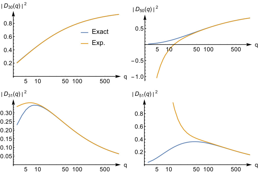 Figure 1
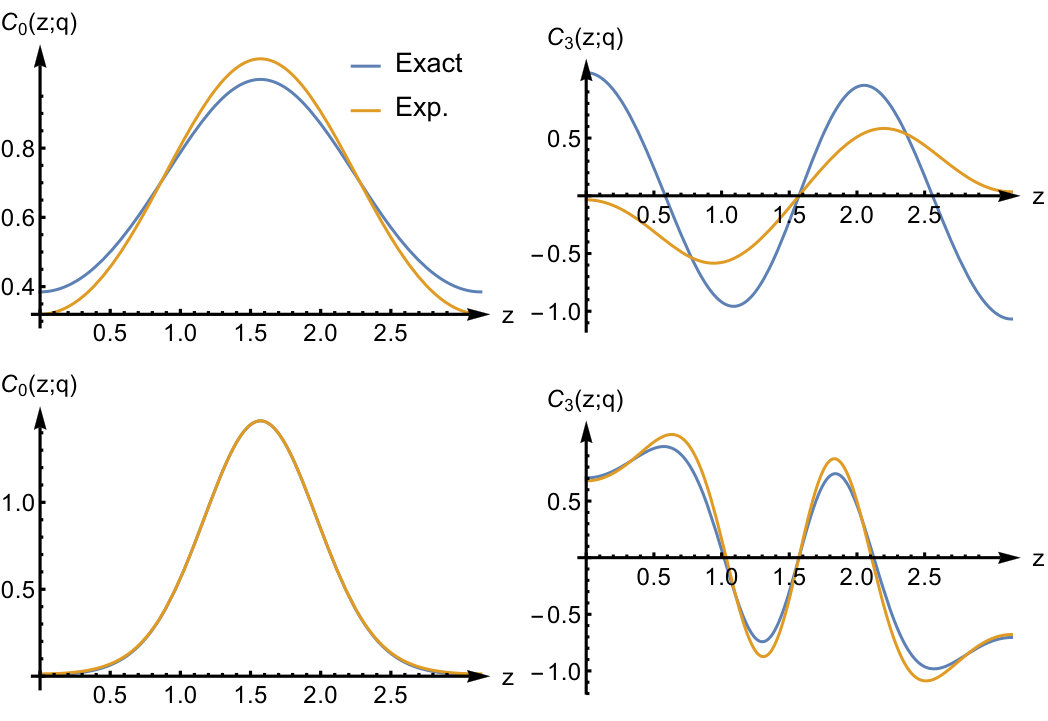 Figure 2
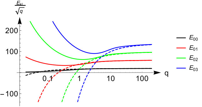 Figure 3
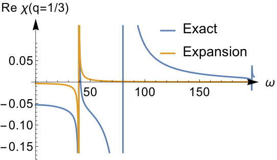 Figure 4
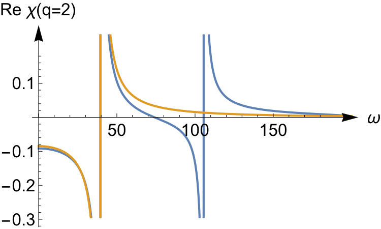 Figure 5
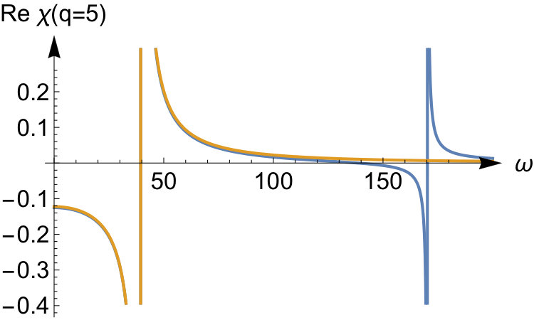 Figure 6
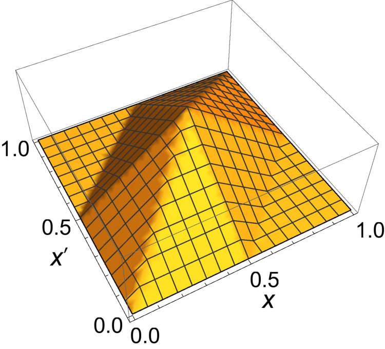 Figure 7
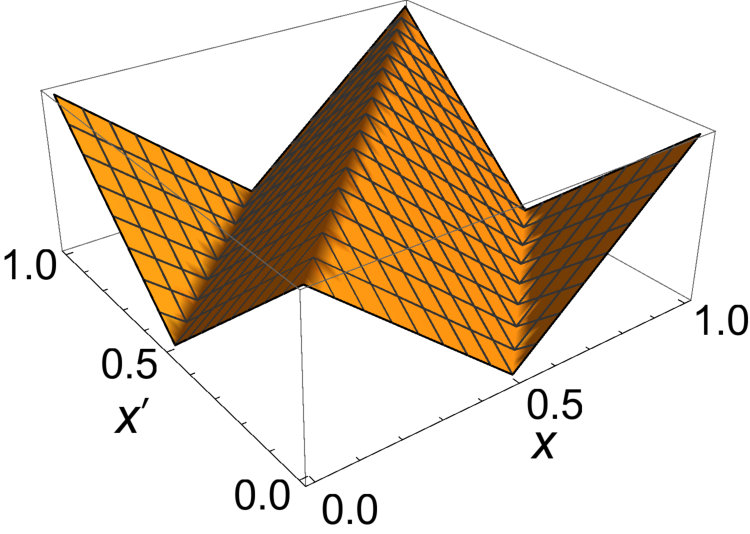 Figure 8
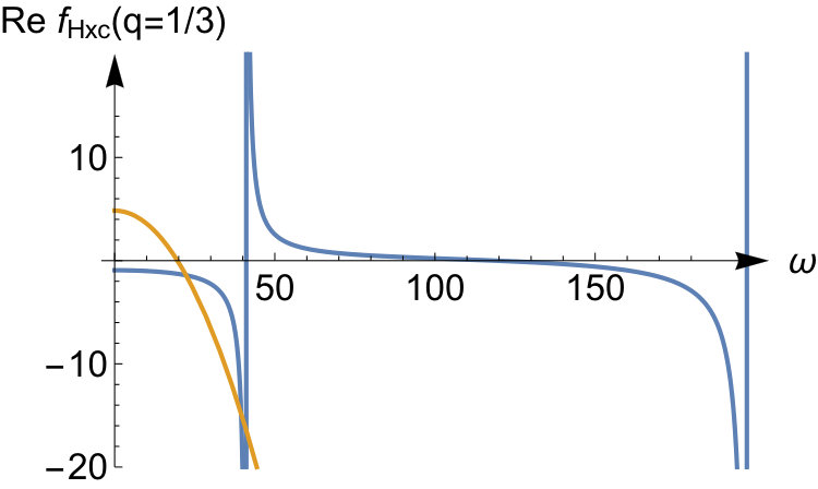 Figure 9
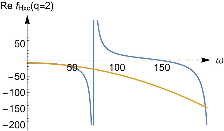 Figure 10
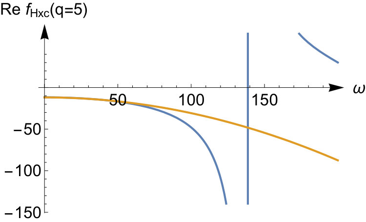 Figure 11
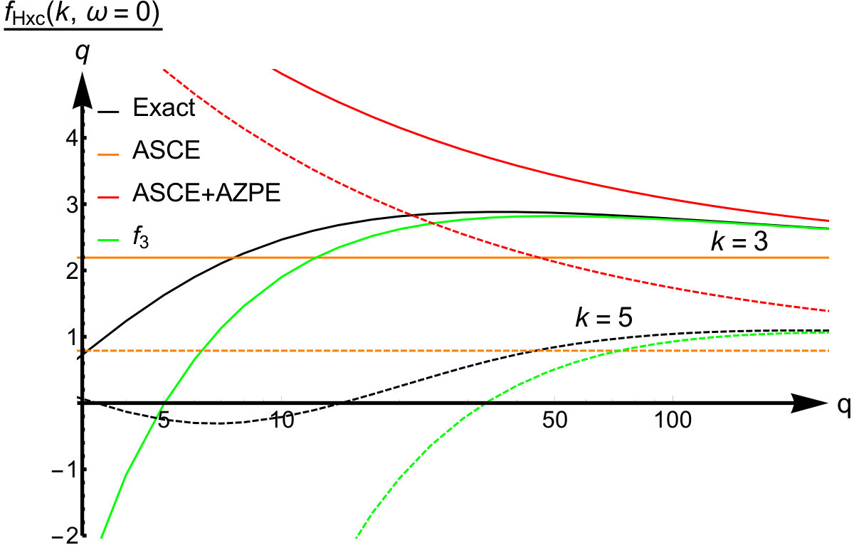 Figure 12
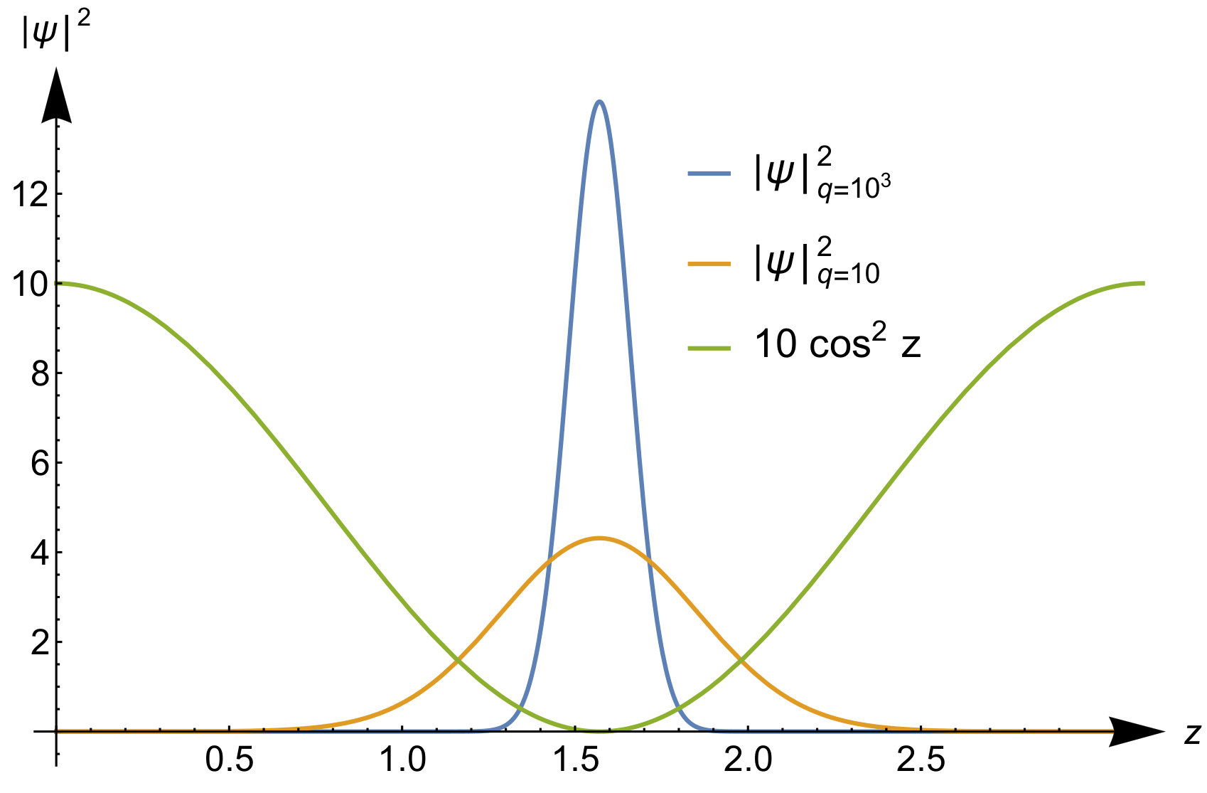 Figure 13
Peer Reviews
No public reviews on file for this paper yet. If you reviewed it on a platform where reviews are public (OpenReview, ICLR, NeurIPS, ICML), you can paste yours below so the community can read it here.
Videos
No videos yet. Explain this paper in a talk, walkthrough, or lecture? Add one.
Time-dependent density-functional theory for strongly interacting electrons
Luis Cort
Department of Physics, Nanoscience Center P.O.Box 35 FI-40014 University of Jyväskylä, Finland
Daniel Karlsson
Department of Physics, Nanoscience Center P.O.Box 35 FI-40014 University of Jyväskylä, Finland
Giovanna Lani
lnstitut de Minéralogie, de Physique des Matériaux et de Cosmochimie, Université Pierre et Marie Curie, 4 place Jussieu, 75252, Paris cedex 05, France
Robert van Leeuwen
Department of Physics, Nanoscience Center P.O.Box 35 FI-40014 University of Jyväskylä, Finland
Abstract
We consider an analytically solvable model of two interacting electrons that allows for the calculation of the exact exchange-correlation kernel of time-dependent density functional theory. This kernel, as well as the corresponding density response function, is studied in the limit of large repulsive interactions between the electrons and we give analytical results for these quantities as an asymptotic expansion in powers of the square root of the interaction strength. We find that in the strong interaction limit the three leading terms in the expansion of the kernel act instantaneously while memory terms only appear in the next orders. We further derive an alternative expansion for the kernel in the strong interaction limit on the basis of the theory developed in [Phys. Chem. Chem. Phys. 18, 21092 (2016)] using the formalism of strictly correlated electrons in the adiabatic approximation. We find that the first two leading terms in this series, corresponding to the strictly correlated limit and its zero-point vibration correction, coincide with the two leading terms of the exact expansion. We finally analyze the spatial non-locality of these terms and show when the adiabatic approximation breaks down. The ability to reproduce the exact kernel in the strong interaction limit indicates that the adiabatic strictly correlated electron formalism is useful for studying the density response and excitation properties of other systems with strong electronic interactions.
I Introduction
Time-dependent density functional theory (TDDFT) Gross et al. (1996); Burke et al. (2005); van Leeuwen (2001); Ullrich (2012); Marques et al. (2012); Ruggenthaler et al. (2015); Maitra (2016) is a well-established approach to study the time-dependent and excitation properties of many-electron systems. One of the main reasons for its popularity is that within this formalism the time-dependent interacting many-body problem can be recast exactly into an equivalent one-particle framework, advantageous for numerical implementations. The corresponding one-particle equations, called the time-dependent Kohn-Sham equations, contain an effective potential, known as the Kohn-Sham potential, which is defined in such a way that the non-interacting system has the same time-dependent density as the original interacting many-body system. The Kohn-Sham potential is typically written as the sum of the external potential of the interacting system and of the Hartree and the exchange-correlation (xc) potential.
In practical applications of TDDFT, the xc-potential is approximated. The type of approximation employed crucially determines the quality of the results, and therefore a considerable amount of research has gone into the difficult task of finding reliable and accurate approximations for this quantity. This task is simpler in the linear response regime where we consider small variations in the density caused by applied perturbations. This regime is of interest as the knowledge of the density response function is sufficient to calculate the excitation energies and the absorption spectrum of the system Petersilka et al. (1996). For this purpose it is enough to know and its functional derivative with respect to the density , evaluated at the ground-state density. The quantity is called the xc-kernel and has been the subject of intense investigations.
The simplest possible approximation is the adiabatic local-density approximation (ALDA) in which the xc-kernel is local in space and time. The ALDA has, however, a number of deficiencies Ullrich (2012) such as, for example, the inability to produce correct charge transfer excitations Stein et al. (2009); Gritsenko and Baerends (2004); Maitra (2005); Autschbach (2009) and Born-Oppenheimer surfaces of excited states in dissociating molecules Gritsenko et al. (2000); Hieringer and Görling (2006); Giesbertz and Baerends (2008) and semiconductor band gaps Botti et al. (2004). Some improvements have been made using hybrid functionals which contain mixtures of exact exchange and traditional local functionals. These methods are non-local in space but still adiabatic. However, they are not systematic and the optimal mixture of exact-exchange is often system-dependent Dreuw et al. (2003); Hofmann et al. (2012); Dierksen and Grimme (2004); Peach et al. (2008). Other, more systematic, approximations for beyond the ALDA often rely on perturbative expansions Görling (1998); Tokatly and Pankratov (2001); von Barth et al. (2005); Fuchs et al. (2005); Hellgren and von Barth (2009, 2010); Heßelmann and Görling (2011a, b); Bates and Furche (2013); Erhard et al. (2016) and many of them are restricted to the exchange-only approximation. Their perturbative nature makes these approaches questionable in the strong correlation regime which is relevant in various physical situations, notably the case of molecular dissociation, and hence it is highly desirable to develop new techniques to tackle this regime.
In a recent work Lani et al. (2016) the so-called strictly correlated electrons (SCE) framework Seidl (1999); Gori-Giorgi et al. (2009); Malet and Gori-Giorgi (2012), a formalism well suited for the description of strong interactions, has been applied within the time-dependent domain. The authors derived an expression for the xc kernel in the so-called adiabatic approximation and established that the adiabatic SCE (ASCE) kernel satisfies the zero force theorem Mundt et al. (2007), an exact property related to generalized translational invariance Vignale (1995a); Dobson (1994). The kernel was furthermore studied for finite one-dimensional systems with different density profiles, some of which are prototypical of the dissociation of two-electron homonuclear molecules. It was found that the ASCE kernel is spatially non-local and exhibits a divergent behavior as the molecular bond is stretched. For adiabatic kernels this diverging behavior is crucial Gritsenko et al. (2000) for describing bond-breaking excitations, which is a notoriously challenging problem in linear response TDDFT. Since the kernel was derived in the adiabatic approximation, not much could be concluded about the limitations of its adiabatic nature in the context of the physics of strong static correlation. The case of infinitely strong electron-electron correlation is quite peculiar and to date it is not known how accurate the adiabatic approximation can be in such a regime.
One way to shed light on this issue is to benchmark the ASCE kernel against an exact expression for obtained from a model system where the density response function and thus the xc-kernel can be calculated analytically. In this work we consider such a model, namely two interacting electrons on a quantum ring Viefers et al. (2004); Ruggenthaler et al. (2012); Loos and Gill (2012); Ruggenthaler et al. (2015), for which not only we compute the exact density response function and xc-kernel, but we also obtain these quantities for various two-body interaction strengths, including the infinitely strong one, and we compare these results with those given by the SCE theory in the adiabatic approximation. The leading order of the asymptotic expansion for the exact and the expression for the ASCE kernel are found to be identical. We also derive the next order correction term beyond the ASCE, called the adiabatic zero-point-energy approximation (AZPE), and show that also this adiabatic term is the same as the next order from the asymptotic expansion. The third order in the expansion for the kernel is still adiabatic, while a frequency dependence appears in the fourth order. In this order, an adiabatic approximation would break down. This is one of the central results of the paper and elucidates both the strengths and the weaknesses of the adiabatic approximation in the limit of strong electron-electron interaction.
The paper is organized as follows. In Sec. II we introduce the quantum ring model and, after computing the full spectrum of its Hamiltonian, we discuss asymptotic expansions for its eigenenergies and eigenstates in the case of strong interactions and analyze them. In Sec. III we study the density response function of strongly interacting systems, while in Sec. IV we focus on TDDFT in the same regime and give an asymptotic expansion for the xc-kernel. Our conclusions are finally presented in Sec. V.
II An exactly solvable system
II.1 Two interacting electrons on a quantum ring
For our study of electron correlations we consider an analytically solvable model, which we will refer to as the quantum ring model, of two electrons on a ring of length which repel each other with a two-body interaction. The interaction strength can be adjusted using a parameter, which allows us to study the exact properties of the system ranging from weak to very strong interactions. The explicit form of the Hamiltonian of the quantum ring is given by:
[TABLE]
where is a dimensionless parameter and has units of energy. The coordinates and are the coordinates of the electrons on the ring which run from [math] to . The ground-state density is spatially constant and independent of ; for this reason the model can be used to illustrate several features of the coupling strength dependence in density functional theory.
In order to calculate the properties of the system we have to determine the eigenfunctions which satisfy the stationary Schrödinger equation where are the energy eigenvalues. For our two-particle system these eigenfunctions can be written as a product of a spatial wave function and a spin function as follows
[TABLE]
For the singlet case (which we will focus on) the normalized spin function is given by
[TABLE]
and is anti-symmetric in the spin variables. For the triplet there are three linearly independent symmetric spin functions which we, for simplicity, all denote by . Since the two-electron wave function is anti-symmetric under the simultaneous interchange of space and spin variables it follows that the spatial wave functions satisfy the symmetry relation
[TABLE]
Apart from these symmetry conditions, the Schrödinger equation needs to be solved with periodic boundary conditions on the variables and , i.e. the wave function and its first spatial derivatives are invariant under the substitution for . Using these conditions we can solve the Schrödinger equation by a suitable coordinate transformation. Since these steps are carried out in detail in Ref. Ruggenthaler et al. (2013) here we just outline the main steps relevant for this work.
The Hamiltonian (1) becomes separable in the terms , the center-of-mass coordinate, and , the dimensionless relative coordinate. This variable transformation gives
[TABLE]
By inserting a product Ansatz of the form into the Schrödinger equation we find that the spatial two-particle eigenfunctions are of the form
[TABLE]
where is an integer and the function satisfies the Mathieu equation which we write in its standard form as Arscott et al. (1964); DLMF
[TABLE]
where the constants and are given by:
[TABLE]
For a given value of the Mathieu equation (3) has only periodic solutions for particular values which are called the Mathieu characteristic values. Moreover this equation has either even or odd periodic solutions which are called the Mathieu cosine and Mathieu sine functions respectively. Both sets of functions form a countable set, therefore its members can be labeled by a non-negative integer . For the Mathieu cosines this label starts at and for the Mathieu sines at . The even Mathieu cosine function is denoted by and its characteristic value by , while the odd Mathieu sine function is denoted by and its characteristic value by . Since the center-of-mass wave functions are symmetric under the interchange of the spatial coordinates of the electrons we see from Eq.(2) that the singlet wave functions must be described by even Mathieu functions whereas the triplet ones must be described by odd Mathieu functions. The final form of the normalized singlet and triplet wave functions therefore is
[TABLE]
in which the normalization of the Mathieu functions is chosen such that
[TABLE]
The Mathieu functions further have the periodicity property , i.e. they are periodic in for even values of and anti-periodic for odd values of . Furthermore the center-of-mass wave function in Eq.(2) changes with a prefactor when , for . Therefore for the wave functions in Eqs.(6) and (7) to satisfy periodic boundary conditions the labels and must be both even or both odd. Note that runs over all integers while only runs over the non-negative integers. From Eq.(5) we see that the energy eigenvalues are given by
[TABLE]
Since in the subsequent discussion of the density response function we focus on the singlet excitations in particular, we write the singlet wave functions in a slightly different form for the purpose of a better interpretation. Multiplying the spatial wave function of Eq.(6) with its singlet spin function, the full space-spin function can be written as
[TABLE]
where we defined the Slater determinant
[TABLE]
and we further defined the spatial normalized orbital by which corresponds to a periodic single-particle wave function of a free particle on the quantum ring. Let us consider the excitation from the ground-state to another singlet state with , which requires that the excited state is characterized by an even value. In that case in the Slater determinant above is a proper periodic wave function as is an integer. According to Eq.(9) the excitation energy is
[TABLE]
which is independent of the interaction strength as the excited state has the same relative wave function as the ground state. For the case that we have and the ground and excited state both become pure Slater determinants. The excitation then represents a promotion of two electrons from a doubly occupied state to a doubly occupied state with a one-particle quantum number , which is commonly called a double excitation. When is non-zero this language is not accurate anymore as also the relative wave function becomes relevant. If the interaction strength becomes very large the energy required to excite to a state with non-zero becomes very large too and the excitations with energy give the dominant contribution to the density response function, as we will see later.
II.2 The strong interaction expansion of the exact solution
As the interaction strength increases, the electronic repulsion becomes more important and the electrons tend to stay in opposite positions on the ring. This physically intuitive picture can be analyzed in more detail using the Mathieu equation. According to Eqs. (6) and (7), the square of the spatial wave function is given by
[TABLE]
where is either a Mathieu cosine or a Mathieu sine depending on whether the wave function is a singlet or a triplet one. We therefore see that the probability to find a given electron at given an electron at only depends on the relative coordinate , as one would expect on the basis of the symmetry of the system. This probability distribution is given by the square of the Mathieu function .
Let us analyze the properties of this function in the large interaction limit which according to Eq.(3) satisfies a single-particle Schrödinger type of equation in a potential of the form . For large values of we can see that the relative wave function described by becomes localized in the minimum of the potential at , which corresponds to a relative distance of the particles of . We can expand the potential around this minimum to obtain
[TABLE]
This potential describes (apart from a shift of the minimum) a harmonic oscillator with frequency . The eigenfunctions of the harmonic oscillator are well known to consist of Gaussians of width proportional to . In the limit of large the harmonic frequency increases and the wave functions become localized around . This behaviour is illustrated in Fig.(1). The eigenenergies of the harmonic oscillator are well-known and given by . This also immediately provides an asymptotic formula for the characteristic value of the Mathieu equation for large values of :
[TABLE]
and consequently also an asymptotic expansion for the eigenenergies of the quantum ring from Eq.(9).
A more rigorous connection to the harmonic oscillator wave functions can be made on the basis of the substitution which transforms the Mathieu equation (3) to the new form
[TABLE]
where we defined and . In the large limit this equation attains the form of the Schrödinger equation for the harmonic oscillator. Its eigenfunctions are well known and, apart from a normalization, are given by the parabolic cylinder functions defined by
[TABLE]
where are the Hermite polynomials. On the basis of this analysis we may suspect that it is possible to find an asymptotic large- expansion of the Mathieu functions in terms of harmonic oscillator functions of argument . Sips Sips (1949, 1959); Blanch (1960); Frenkel and Portugal (2001) already derived such an expansion on the basis of the transformed Mathieu equation. For reference in the next section we briefly outline its main features for the case of the Mathieu cosine which is relevant for the discussion of singlet states. The general form of the Sips expansion is given by
[TABLE]
in which we defined . The specific form of the coefficients is given in the work of Sips Sips (1949, 1959); Blanch (1960) who outlined a systematic procedure to obtain them. In general they can be obtained from a recursion relation Frenkel and Portugal (2001) and we refer to Appendix B for a more detailed discussion.
In Eq.(13) we see that for odd values of the Mathieu cosine is expanded in functions with only odd values of while for even it is expanded in functions with only even values of . This follows directly from the derivation by Sips Sips (1949) but we see with hindsight that this condition is necessary to make the Mathieu cosine satisfy . Namely, if we replace by then the variable changes to yielding this desired property for a series of the form (13) since . The Sips expansion, Eq.(13), will be used in the next section to determine the large interaction expansion of the density response function.
We conclude the section with a remark on the eigenenergies of the quantum ring. We can obtain an asymptotic expansion for them as the work of Sips also derives the large behavior of the Mathieu characteristic values in terms of an asymptotic series expansion in power of (see Appendix B). Taking the first few leading orders we obtain the following expression for the eigenenergies of the quantum ring
[TABLE]
The asymptotic expansion is the same for the singlet and triplet energies as their difference becomes exponentially small in the large limit (see Appendix B). To illustrate the -dependence of the eigenenergies we present in Fig. 2 some of the lowest eigenvalues and their asymptotic expansion from Eq.(14) as a function of . We see that the asymptotic expansion converges more slowly for higher values of , and for these we need high values of in order to have a reliable estimate.
III Density response of strongly interacting electrons
After having discussed the two-particle wave function and energy spectrum of the system, let us now move to its response properties. Particularly relevant to TDDFT is the induced density change when a small time-dependent external potential is applied. They are related by the retarded density response function as follows
[TABLE]
where is defined via
[TABLE]
where is the density operator in the Heisenberg picture and is the ground state of the system. Since the unperturbed system is time-independent, the density response function is a function of the relative time only and we can Fourier transform it with respect to :
[TABLE]
Before addressing in greater detail the properties of of the quantum ring in the large interaction limit, let us first make some considerations about the static density response function in a more general context.
III.1 Static density response in the strong interaction limit
Let us consider an interacting many-electron system in its ground state. The Hamiltonian consists of a kinetic energy operator, an external potential and a two-body interaction. If we consider a small variation in the static external potential, the ground-state density will vary by an amount which can be expressed as
[TABLE]
where is the static density response function. Let us now consider a shifted potential . The ground-state density for this new potential is given by . For small translations we can write that and similarly . Since this is valid for all small vectors we find from Eq.(17) that
[TABLE]
This equation relates the gradient of the external potential to the gradient of the ground-state density, and amounts to the static limit of an equation derived for the dynamic density response function by Vignale Vignale (1995b).
Let us now consider a system in which we scale the two-body interaction with a parameter and let us choose the external potential in such a way that the density is the same for all values of . According to the Hohenberg-Kohn theorem Hohenberg and Kohn (1964) such a potential is unique when it exists. For such a system the density response function will depend on as well and Eq.(18) becomes
[TABLE]
Let us now consider the limit of very large values of . One can show, for a general inhomogeneous system, that asymptotically where is the so-called strictly-correlated electron potential Seidl (1999); Seidl et al. (2007); Gori-Giorgi et al. (2009). The result is intuitively clear as the linearly growing repulsive two-body interaction must be compensated by a linearly growing attactive one-body potential in order to keep the density profile constant. This has consequences for the behavior of . We consider two cases. Let us first assume that for the response function attains a finite value . Because the left-hand side of Eq.(19) is independent of this implies that
[TABLE]
which means that the three vector components of must be eigenfunctions of with zero eigenvalue. Since the density response function reaches a finite limit the system does not become rigid even when the interaction becomes infinitely large. This is a possible situation in systems in which the Hamiltonian by a coordinate transformation can be separated in two parts in which one of the parts is weakly dependent on the interaction strength. That such inhomogeneous systems exist is demonstrated for the harmonic model system described in Appendix A and for which we demonstrate that Eq.(20) is indeed valid.
A probably more common situation is that such a separation is either not possible or that both parts of such a Hamiltonian are still strongly -dependent. In this case one would expect that the energy required to excite the system grows with , and as such the density response function would vanish for large . If this is the case it is to be expected that in Eq.(19) asymptotically behaves as
[TABLE]
where is a -independent function and the terms that follow decay faster than . This means that for a given perturbation the density response decays as and therefore the strong interaction makes the system more rigid and suppresses density variations. In such a case Eq.(19) reduces to
[TABLE]
which is an exact equation for the leading order in .
When we finally consider systems in which the ground-state density and external potential are spatially constant, the reasoning that we carried out does not apply anymore since the gradients in Eq.(19) are identically zero. However, such systems are homogeneous which implies that the center-of-mass can be separated off and we can therefore expect the response function to attain a finite value in the large interaction limit. This is exactly the case of our quantum ring model. Indeed we saw in Eq.(11) that the quantum ring admits excitation energies that are independent of the interaction strength and these correspond to excitations that only change the center-of-mass wave function and do not affect the relative probability distribution of the particles. As we will see in more detail below, such excitations give a contribution to the density response function that survives in the large interaction limit, while the remaining excitations give a contribution which behaves as in Eq.(21).
It is interesting to connect this analysis to the -sum rule for the dynamic density response function. In a system where the density is kept independent of with the -sum rule attains the form Stefanucci and van Leeuwen (2013)
[TABLE]
We therefore see that the frequency integration removes the -dependence. This is not in contradiction with Eq.(21). Although the density response function itself can become very small for large the integrand in Eq.(23) can remain finite as it is weighted by the frequency . As a consequence the integral gets contributions proportional to the excitation energies which grow with increasing interaction strength.
III.2 Exact density response of the quantum ring
After having discussed the general static case, we now turn our attention to the exact dynamical density response function of the quantum ring. Inserting a complete set of eigenstates of the Hamiltonian from Eq.(1) into the one-dimensional analogue of Eq.(16) we find the Lehmann representation Stefanucci and van Leeuwen (2013) of the retarded response function
[TABLE]
where we defined the excitation energies as . The expression contains an infinitesimal parameter that arises from the Fourier transform of the Heaviside function and the limit is implied after the evaluation of all terms. Furthermore is the density operator in the Schrödinger picture and labels the singlet or triplet eigenstates. The label runs over all positive and negative integers while runs over non-negative integers, with the condition that both are even or both are odd. The expression in Eq.(24) is simplified by the fact that the triplet terms vanish because the triplet spin-function is orthogonal to the singlet spin function of the ground state, which yields . The remaining non-zero terms can be evaluated as
[TABLE]
where denotes the spatial part of the singlet wave function of Eq.(6) expressed in the original coordinates and the excitation amplitudes read
[TABLE]
The amplitude has a number of properties directly related to properties of the Mathieu functions. Since is real, , and as a consequence of the orthogonality of the Mathieu functions, . Moreover, the fact that and that these functions are even in leads to . Making use of the symmetry properties of described, combined with , yields the following expansion of the response function
[TABLE]
where
[TABLE]
in which the sum runs over even values of for even and over odd values of for odd. We see from Eq.(27) that can be regarded as the discrete Fourier transform of with respect to the relative spatial coordinate as was to be expected on the basis of the symmetry of the system. It will be now convenient to define the spatially discrete and temporally continuous Fourier transform of a function and its inverse as:
[TABLE]
By using this Fourier transformation in Eq.(15) we rewrite the density response as
[TABLE]
in which is an integer and a continuous variable. We will make use of this relation below. We have now obtained an explicit form of the density response function that allows for an analytical analysis in the strong interaction limit.
However, before moving to that, we briefly give the form of the response function for the non-interacting system, i.e. , which in the density functional context will be the same as the Kohn-Sham response function, since the system has the same density for all values of . For the noninteracting case the Mathieu characteristic value is and the Mathieu cosine functions are given by and for . The excitation energies are given by Eq.(9),
[TABLE]
while the eigenstates are given by Eq.(6) as
[TABLE]
in which is always even. Note that yields a doubly excited state. The corresponding excitation amplitude can be calculated from Eq.(26). Apart from the amplitude , which does not contribute to the Lehmann sum since , for we have that
[TABLE]
Since only terms where is even contribute, we see that the only non-zero excitation amplitudes are the ones with . This implies the absence of double excitations in the density-response function, a well-known property of non-interacting systems Maitra et al. (2004); Ullrich (2012). Inserting Eq.(33) into Eq.(28) we find that the non-interacting response function is given by
[TABLE]
with . We note that in -space, has only a single pole for , and no zeroes.
Having determined the non-interacting response function, it now remains to study the density response function in the complementary limit of very strong interactions. For this purpose we need to study the excitation energies and excitation amplitudes in the limit of large . This is the topic of the next section.
III.3 Strong interaction expansion of the dynamic density response function
Let us focus on the excitation energies and the excitation amplitudes for large . Because for explicit asymptotic expansions are known (see Appendix B), this leaves us with the determination of defined by Eq.(26). We start by inserting the Sips expansion of Eq.(13) into Eq.(26), which gives
[TABLE]
where we defined
[TABLE]
where . Since the coefficients are known (see Appendix B for explicit expressions) it remains to evaluate . Changing the integration variable to and defining gives the expression
[TABLE]
where we defined the function
[TABLE]
and its Taylor coefficients . Inserting this Taylor series into Eq.(37) then gives the expansion
[TABLE]
where the interchange of integral and sum is allowed as we have an absolutely convergent series. Due to the Gaussian decay of the functions , in the limit , we make an error which, as a function of , decays faster than any polynomial function if we replace in the limits of the integral by infinity. We therefore obtain the asymptotic expansion
[TABLE]
where we introduced coefficients of the form
[TABLE]
This integral can be computed analytically, and the explicit expression is given in Appendix C. Also note that due to the parity properties of the integrand vanishes unless and are both even or both odd. Therefore, depending on whether is even or odd, the summation index in Eq.(39) can be taken to run only over even or only over odd values.
Expression (39) together with Eq.(35) gives an explicit procedure to calculate the large expansion of the excitation amplitudes. The asymptotic expansions of and of are given in Appendix C in Eq.(105) and Eq.(106) respectively. Together with the asymptotic expansion for the excitation energies, Eq.(97), inserted into Eq.(28) we find that the asymptotic expansion of the density response function is given by
[TABLE]
From this expression, we can draw a number of interesting conclusions. We find that the response function behaves quite differently for even and odd Fourier coefficients in the strong interaction regime. If we apply a potential with general coefficients to the system, the density change is strongly suppressed for odd as becomes very small. In this limit it will therefore mainly have even Fourier coefficients which implies that i.e. the density change at antipodal points of the ring is the same. If we however apply a potential with only odd Fourier coefficients the density change has the symmetry and is therefore opposite in antipodal points of the ring. From Eq.(41) we find that the leading term in real space in this case is given by
[TABLE]
We can understand the dependence on as follows. The generation of an anti-symmetric antipodal density requires excitation to states with an odd number of nodes in the relative wave function which requires a large energy in the strong interaction limit and therefore the density response is suppressed for large interaction strength. From Eq.(42) we also see that the density increases instantaneously around the points were the potential has positive curvature. The instantaneous nature of the response has a simple explanation. If we perturb the system with a potential which is only non-zero for frequencies well below the first excitation energy, the temporal variation of the perturbation is much slower than a typical timescale of the free evolution of the system and the density response can be regarded as instantaneous. Since the excitation energies for odd (which must have odd as well) increase proportionally to the density response function in this case is well approximated by a frequency independent function for , which explains the instantaneous dependence of the density variation on the perturbation in Eq.(42).
For even values of the density response function has a more interesting frequency dependence. In the strong interaction limit
[TABLE]
The poles of this response function correspond to the center-of-mass excitations of Eq.(11). Being independent of they are not shifted towards infinity when we increase the interaction strength. This is a peculiarity of the quantum ring system as the Hamiltonian is separable in a -dependent and a -independent part. This happens also for some other homogeneous systems such as the three-dimensional electron gas with periodic boundary conditions or for electrons restricted to the surface of a sphere Seidl (2007). The analysis based on Eq.(19) shows that such a separation is usually not possible in inhomogeneous systems. When it is possible, both parts will generally still depend on (see Appendix A for an example).
To illustrate the accuracy of the expansion in Eq.(41) we display the exact response function and the expanded one in the top panels of Fig.3 for and for some values of the interaction strength. For small interactions the exact response function has two poles; one is approximately at the same location as the Kohn-Sham response function , while a new pole with a small weight appears at the center-of-mass excitation energy at . The expansion captures this pole, albeit with a very different weight. When we increase the interaction strength, the pole originally at the Kohn-Sham energy will shift to higher energies to a position proportional to , while the pole corresponding to the center-of-mass excitation stays fixed and increases in weight. Already at , the asymptotic expansion yields good results for this -value. We thus see that the expansion is accurate for frequencies that are small compared to . This result was to be expected since in the expansion of Eq.(41) we treated the frequency as a constant that is small compared .
Having obtained the exact response function we have obtained all information needed to study the xc-kernel of TDDFT, which will be the topic of the next section.
IV TDDFT in the strong interaction limit
IV.1 The exchange-correlation kernel
In TDDFT an effective non-interacting system, known as the Kohn-Sham system, is constructed in such a way as to have exactly the same density as the interacting many-particle system of interest. The external potential in this system, , is a functional of the density Ruggenthaler et al. (2013, 2015) and is often written as follows
[TABLE]
Here is the external potential of the interacting system of interest and the two-particle interaction of that system. The second term in Eq.(44) is the Hartree potential and the last one is the exchange-correlation (xc) potential. Taking the functional derivative of Eq.(44) with respect to the density one obtains
[TABLE]
Here is the inverse of the Kohn-Sham density response function whereas is the inverse of the density response function of the interacting system and , the Hartree-xc kernel, is defined as
[TABLE]
where is the sum of the Hartree and the xc-potential. Equation (45) is commonly used to calculate from the knowledge of at the price of approximating .
For the discussion in the next section it is important to note that the functional derivative is not a uniquely defined function Hellgren and Gross (2012); Ruggenthaler et al. (2013) due to the fact that for a system with a fixed number of particles the density change must integrate to zero at any time, i.e.
[TABLE]
Let us define a new function
[TABLE]
with and arbitrary functions. The change in the Hartree-xc potential produced by the kernel of Eq.(48) due to a density change is given by
[TABLE]
where the integral over integrates to zero as a consequence of Eq.(47) and the integral over yields a function of time only, which is merely a gauge of the potential. We therefore see that and are physically equivalent integral kernels. The quantity that is defined unambiguously 111Note that Ref. Lani et al. (2016) did not discuss the possible addition of arbitrary functions of one spatial variable to the kernel. is the mixed spatial derivative
[TABLE]
a property that will be used below.
Let us turn to the specific case of the quantum ring. The density response function is diagonal in the momentum-energy representation and for the Fourier components the following relation holds:
[TABLE]
By Fourier transforming the kernel we impose a dependence on the relative coordinate in real space, which reduces the ambiguity of Eq.(48) to that of adding an arbitrary spatially constant function. In Eq.(51) this freedom is reflected in the fact that the kernel is well-defined for all -values except for , since in this case both the response functions vanish. For the homogeneous quantum ring the Kohn-Sham response function coincides with the response function of truly non-interacting electrons of Eq.(34). Using this equation, together with the expansion of Eq.(41), we obtain an explicit expression for in the strong interaction limit:
[TABLE]
where we have reintroduced the variable rather than as the notation is commonly used in the density functional context, which will be central for the discussion in the next section. Since these quantities only differ by a numerical prefactor (see Eq.(4)) we will refer to the large interaction regime as the regime in which either of these two variables tends to infinity.
To illustrate the accuracy of the expansion in Eq.(52) we display the exact kernel and the expanded one in the bottom panels of Fig.3 for and some values of the interaction strength. We see that the corresponding asymptotic expansion for is accurate up to the lowest excitation energy corresponding to a change in the relative wave function. In this energy region has a pole at an energy corresponding to a zero in , as a consequence of Eq.(51). It is worth noticing that, since the non-interacting response function has no zeroes, there is no pole in originating from the first term in Eq.(51). This is peculiar to our quantum ring system for which the non-interacting response function has only a single pole for . Instead, for a general system, the Kohn-Sham response function will have multiple poles and zeroes which implies that, to order , is frequency dependent causing the adiabatic approximation to fail in this order. In our system for even tends to a frequency-independent function for all when the interaction strength approaches infinity. Its static value, given by , is the value needed to shift the Kohn-Sham pole to the pole.
For the odd values (not shown here), all poles in the response function shift to infinity as . The asymptotic expansion for captures this, and the kernel becomes frequency-independent in this limit. In fact, for odd values of in Eq.(52), all the leading terms up to order are frequency independent. However, frequency-dependent terms will appear to order (not presented here) as is also the case for even .
For the discussion in the next section it is useful to recast the kernel in real space. The expressions in Eq.(52) are sufficient to calculate this quantity to order in real space using the Fourier transform of Eq.(53)
[TABLE]
and is the relative distance between the points and which are the one-dimensional counterparts of the spatial points in Eq.(46). Since and are both in the interval from [math] to we have that . We find that
[TABLE]
The leading term is given explicitly by
[TABLE]
in which we choose the arbitrary constant function (see the discussion below Eq.(51)) such that the Fourier coefficient of becomes zero for . For we find (up to a constant) that
[TABLE]
Since in the next section we will focus mostly on and , we do not report here the real space representation of . In the next section we will show how and can be calculated in an alternative manner using the SCE theory in the adiabatic approximation.
IV.2 Expanding the xc-kernel in the theory of strictly correlated electrons
To date, no good and reliable approximations for electrons in the strong correlation regime have been developed within TDDFT. A ground-state theory of so-called strictly correlated electrons (SCE) Seidl (1999); Seidl et al. (2007) has been constructed and applied within the adiabatic approximation to calculate the xc-kernel to the leading order in the interaction strength. In this section we will first benchmark this approximation against the exact solution for the quantum ring model, and then derive and compare the next order.
Let us begin with a brief overview of the ingredients of SCE theory that we will use. The Hartree-xc energy for a system with interaction strength can be written as Langreth and Perdew (1975):
[TABLE]
where we defined:
[TABLE]
In this expression is the two-particle interaction and is the ground-state wave function of a system with a local external potential, interaction and ground-state density . In the strong interaction limit can be expanded asGori-Giorgi et al. (2009),222Strictly speaking the absence of a term of order in this expansion has only been shown for a Coulomb system but we find it to be true in our model as well:
[TABLE]
where the first term is the SCE energy which has the explicit form:
[TABLE]
where is the two-particle interaction which we assume to depend only on the distance between the particles. The functions are the so-called co-motion functions, which specify the position of electrons given the position of one electron at . The second term in Eq.(59) contains the so-called zero-point energy (ZPE) which describes the vibrations of the electrons around their equilibrium positions and is given explicitly as:
[TABLE]
where is the spatial dimensionality of the system and are the harmonic frequencies. Inserting Eq.(59) into Eq.(57) we find the large expansion of the Hartree-xc energy to be:
[TABLE]
The ground-state theory can be used in the adiabatic approximation Lani et al. (2016) to find an approximate exchange-correlation kernel from
[TABLE]
where we added the superscript A to indicate that we make the adiabatic approximation. This approximation yields a frequency independent Hartree-xc kernel when transformed to frequency space, which we denote as . The second order variation of Eq.(62) with respect to the density gives an expansion in orders of for the Hartree-xc kernel:
[TABLE]
where we defined the adiabatic SCE and ZPE kernels as
[TABLE]
Let us now turn again to the case of the quantum ring. In this case there are two electrons and just one simple co-motion function given by
[TABLE]
If one electron is at this function simply puts the other electron at the antipodal point of the quantum ring. From this co-motion function it is straightforward to calculate the SCE energy. Since we have from our interaction in Hamiltonian (1) that and therefore for our density. Physically this means that the electrons are simply localized at the bottom of a potential well with zero energy.
To next order oscillations around these equilibrium positions start to appear. These zero-point oscillations give an energy contribution which can be calculated using Eq.(61). For a one-dimensional two-electron system there is only one non-zero harmonic frequency given by Malet et al. (2014)
[TABLE]
where . If we calculate this frequency for our quantum ring we find and . We can verify that this is in accordance with the exact strong interaction expansion of the Hartree-xc energy. Since the Kohn-Sham kinetic energy as well as the external potential is zero for the quantum ring system, simply coincides with the total energy, which is known in the strong interaction limit from the large- expansion of the lowest Mathieu characteristic value (see Appendix B). This gives
[TABLE]
where the leading coefficient indeed exactly gives . The expansion of can be calculated from Eq.(57) to give
[TABLE]
This result agrees with a direct calculation of using the Sips expansion of the Mathieu functions and indeed has the structure of the expansion in Eq.(59) in which we also included the term to order .
Let us turn to the calculation of the kernels of Eqs.(65) and (66).
The ASCE kernel is obtained from the expression derived in Ref. Lani et al. (2016) and reads
[TABLE]
where is the function given in Eq.(55). Because of the freedom in Eq.(48) is physically equivalent to the kernel and agrees with the leading term in the expansion of Eq.(54) in the strong interaction limit. Both kernels are shown in Fig.4. Since has a simpler shape, we will restrict ourselves to this function. The kernel describes how a density variation induces a change in . To leading order in we have
[TABLE]
By taking the second derivative of this equation, we obtain
[TABLE]
where we stress that is periodic with . Since is linear everywhere except at the kinks at , the second derivatives yield delta functions at these points. Also note that the sign of the density change yields the curvature of the induced potential. Eq.(72 ) has some interesting consequences. If we make a localized density variation in a very small interval of the ring, there will not only be a change in the same interval, but at the same time a similar change in the potential with opposite sign in an antipodal interval. This shows very clearly that the Hxc-potential depends non-locally, but instantaneously, on the density.
Let us analyze the next orders in the strong interaction expansion. The calculation of allows for a comparison with the next leading term in Eq.(54) which is proportional to . The kernel was obtained by taking the second functional derivative of the one-dimensional counterpart of Eq.(61), using Eq.(68) and the functional derivative of the co-motion functions (derived already in Ref. Lani et al. (2016)). We also find agreement between this expression and that of the next leading term in Eq.(56), i.e. modulo the addition of arbitrary functions of and separately (see again Eq.(48)). We observe that the first two leading terms of the expansion of the Hartree-xc kernel from the adiabatic SCE theory agree with the exact results for the quantum ring. An interpretation of this fact will be presented below.
We have thus seen that, in this model, the ASCE and AZPE terms agree with the terms and respectively of the exact asymptotic expansion. To better elucidate their role in the strong interaction limit, we show in Fig. 5 the first three terms contributing to , all scaled by , and compare them with the expression for the exact kernel, in Fourier space for and . As was pointed out earlier the accuracy of the expansion depends on the value of : high -values require higher values to achieve better accuracy. The first term, that is the ASCE, is constant, while the second one, that is the AZPE, only improves on it for large -values and worsens it for smaller ones, as one would expect for an asymptotic expansion. The third term, beyond the AZPE, also exhibits a non-negligible contribution in the small- regime.
We will now offer a physical interpretation of the above terms and make some considerations about their properties in the case of more general systems than the quantum ring model. In the (infinitely) strong interaction limit, a given system behaves very rigidly, since the position of the reference electron determines the positions of all the remaining electrons. Upon application of a perturbation, the response of the system is instantaneous, or adiabatic, while maintaining its rigidity, unless special symmetries are present. This behavior is likely to apply to a wider class of systems, both with a uniform (such as the quantum ring) and a non-uniform density. On the other hand it is unclear whether the frequency-independence of is equally general as we already move away from the strictly correlated electron limit by introducing zero-point vibrations: thus the adiabaticity of for general systems is still an open issue. Finally, as already noted before, the third term of the expansion will be non-adiabatic for general systems.
V Conclusions
In this work, we have considered an exactly solvable model consisting of two interacting electrons on a quantum ring. We focused on the response properties and calculated the energy spectrum, the excitation amplitudes, the density response function, and the exchange-correlation kernel of time-dependent density functional theory. In the limit of strong interaction, we developed an asymptotic expansion in powers of the square root of the interaction strength for the response function and kernel. For the kernel we found that its leading terms are local in time but non-local in space. This already shows that the commonly used adiabatic local-density, or semi-local, approximations will fail for such strongly correlated systems, since they are local both in time and space. We compared the expansion for the kernel to a similar one obtained from the adiabatic-SCE formalism Lani et al. (2016) which has the spatial non-locality built in. The leading term of the exact expansion was found to coincide with the adiabatic-SCE kernel derived in Ref. Lani et al. (2016). After working out the next order term, the so-called zero-point energy contribution, we found that it also coincided with the exact next-to-leading term. For our model, the subsequent term in the expansion is still adiabatic, but we showed that in general systems this term will be non-adiabatic.
The agreement with our exact results puts the adiabatic-SCE and the adiabatic-ZPE approximations on firmer ground and gives confidence in employing the formalism of strictly correlated electrons in the adiabatic approximation for calculating response properties of strongly correlated systems.
Acknowledgements.
LC, DK and RvL acknowledge the Academy of Finland for support under project no. 267839. GL acknowledges the Université Pierre et Marie Curie through an ATER position, which granted her considerable flexibility and freedom to contribute to this work.
Appendices:
Appendix A Response function of a harmonic model system
To illustrate some properties of the response function in the large interaction limit for an inhomogeneous system, let us analyze a model system of two harmonically confined electrons in three dimensions with a harmonic repulsionMoshinsky et al. (1970). The Hamiltonian of the system is given by
[TABLE]
in which the harmonic frequency is chosen in such a way that the density is independent of . Using the coordinate transformation and the Hamiltonian can be written as that of two independent harmonic oscillators
[TABLE]
where . The eigenfunctions and eigenvalues of this Hamiltonian are well-known. The normalized eigenfunctions are given by
[TABLE]
where we defined the triplet of non-negative integers and and the functions
[TABLE]
in which we denoted
[TABLE]
where and is the Hermite polynomial of order . The energy eigenvalues are given by
[TABLE]
The ground-state wave function has the explicit form
[TABLE]
From this function the density is readily obtained as
[TABLE]
where we defined
[TABLE]
If we insert into this relation, we can determine the -dependence of as is independent of . We find
[TABLE]
where solves the quartic equation
[TABLE]
In the limit of large interaction we find that such that
[TABLE]
We see that the harmonic frequency of the center-of-mass mode approaches infinity whereas the one of the relative mode approaches a finite value. This has interesting consequences for the excitation spectrum. For the excitation energies of the relative mode it implies that
[TABLE]
while all other excitation energies diverge to infinite values at large interaction strength. The latter correspond to excitations of the center-of-mass mode. In contrast to the quantum ring, only the excitation energies of the relative mode remain finite in the large interaction limit which is due to the very different nature of the two-body interaction.
Let us turn our attention to the density response function. In the response function only the singlet excitations contribute. This means that the spatial wave functions that we need to consider are symmetric in the interchange of the particle positions. For this to be true, the relative wave functions need to be even and we have to require that only attains even values. The response function therefore has the form
[TABLE]
where are the excitation energies and we further put the restriction that we sum over all such that is even. The excitation amplitudes corresponding to these excitations are given by
[TABLE]
where we rewrote the eigenfunctions in terms of the original coordinates. Let us now consider the large interaction limit of the response function. Since only the excitation energies of the form remain finite in this limit we only need to consider the excitation amplitudes of the form
[TABLE]
If we now use that
[TABLE]
is a limit representation for the delta distribution and the fact that in the large interaction limit we find that
[TABLE]
For the response function in the large interaction limit we therefore obtain
[TABLE]
where the sum runs over values such that is even. We see that in the large interaction limit it is still possible to excite the relative modes of the system.
Let us now have a look at the external potential in the strong interaction limit
[TABLE]
which implies . Since the response function does not vanish in the large interaction limit, Eq.(20) tells us that
[TABLE]
must hold, where we took the static limit of the response function of Eq.(92). Since the polynomial functions in Eq.(92) are all even (since is even), and is an odd function, we find that this relation is indeed satisfied.
Appendix B Sips’ expansion of the Mathieu function
In this Appendix we describe the details of the expansion of the Mathieu functions for large . A recent general discussion is given by Frenkel and Portugal Frenkel and Portugal (2001) who give an overview of various expansions for the Mathieu functions for large and small values of in different regions of their domain and recursion formulas to determine the expansion coefficients. The expansion that we are interested in for this work is the large expansion for the Mathieu cosine function in the region enclosing the value . Such an expansion was derived originally by Sips Sips (1949, 1959); Blanch (1960); DLMF who developed a systematic theory. For the Mathieu cosine this expansion is of the form of Eq.(13). We here give the explicit expressions for the coefficients in Eq.(13), and for this it will be convenient to define new coefficients
[TABLE]
which only differ from the coefficients by a prefactor . This is done to ensure that , which is convenient for a recursive calculation of the remaining coefficients as is done in Blanch (1960); Frenkel and Portugal (2001). The prefactor is chosen such that the Mathieu cosine satisfies the normalization of Eq.(8). It has the explicit asymptotic expansion Sips (1949); Blanch (1960); Frenkel and Portugal (2001)
[TABLE]
In terms of the new coefficients the Sips expansion of Eq.(13) becomes Blanch (1960)
[TABLE]
where the functions are defined in Eq.(12) and . Note that the expansion here differs in the choice of argument compared to that of Ref. DLMF by a factor of as we preferred to use the physicist’s convention for the Hermite polynomials appearing in the harmonic oscillator functions . We prefer here to avoid a general discussion on the determination of and refer the interested reader to Refs. Blanch (1960); Frenkel and Portugal (2001) for details. Instead we give the explicit forms of the coefficients up to order which is sufficient for this work:
[TABLE]
where we define if . From the formulas given in Ref. Frenkel and Portugal (2001) it is readily seen that to know the Sips expansion to order we need to know the coefficients for . For example, the knowledge of the next order would need the knowledge of the coefficients from up to , see for example Blanch (1960).
To show the accuracy of the Sips expansion we display in Fig.6 the Mathieu cosine for and for and and compare them to the Sips expansion using the coefficients given explicitly above. We see that already at the Sips expansion performs very well. In general we find that for higher values of more terms in the expansion need to be taken into account for high accuracy.
It remains to give the asymptotic values of the Mathieu characteristic value. The characteristic values and have the same asymptotic expansion of the form Frenkel and Portugal (2001)
[TABLE]
while the difference is exponentially small in the large limit DLMF .
Appendix C Expansion of the excitation amplitudes
Here we further outline some general features of the expansion of the excitation amplitudes . If we rewrite the expansion of Eq.(35) using the coefficients of Eq.(94) we have the expression
[TABLE]
For the products of the pre-factors we can write
[TABLE]
where has an expansion in powers of , i.e.
[TABLE]
and higher powers can be calculated from expression (95). With these definitions and Eq.(39) we can rewrite the expansion of Eq.(98) as
[TABLE]
where the factor from Eq.(99) has been absorbed in the last sum. The function and the coefficients have an expansion in powers of . Now since the coefficients vanish unless and are both even or both odd, we conclude that has an expansion only in odd powers of if is odd and only in even powers of otherwise. The explicit expression for is given by
[TABLE]
where we defined Weisstein . Finally the coefficients can be obtained from a Taylor expansion of the function defined in Eq. (38). Taken all these terms together we find the following expansion of the excitation amplitude:
[TABLE]
The excitation amplitude indeed has an expansion in odd powers of for odd and in even powers of for even , as we demonstrated above. This implies that has an expansion in powers of . The expansion derived here has been checked numerically to ensure the correctness of the derivations. As a further check on the result we see that the excitation amplitude satisfies as well as .
The order for given in Eq.(105) is enough to yield the following asymptotic expansion for the absolute value squared of the excitation amplitudes to order
[TABLE]
We compare the expansion of to the exact values obtained by numerically integrating Eq.(26) in Fig.7. We see from this figure that higher values of require higher values of to make the expansion accurate. This was to be expected since larger -values imply a more oscillatory integrand in Eq.(26) while a larger value of makes the Mathieu functions more localized and thereby making the expansion of Eq.(38) used in the integrand more accurate.
We finally note that the frequency-sum rule, Eq.(23), can be used to check the validity of some of the terms of Eq.(106). If we insert the explicit form of Eq.(28) into the one-dimensional equivalent of Eq.(23) for the frequency sum rule we can derive that
[TABLE]
where the sum runs over even if is even and over odd when is odd. The right hand side is independent of the interaction strength , thus in the sum on the left hand side the -dependence in the excitation amplitudes has to be compensated by the -dependence of the Mathieu characteristic values to give a result independent of the interaction strength.
The reference list from the paper itself. Each links out to its DOI / PubMed record.
- 1Gross et al. (1996) E. K. U. Gross, J. F. Dobson, and M. Petersilka, “Density functional theory of time-dependent phenomena,” in Density Functional Theory II: Relativistic and Time Dependent Extensions , edited by R. F. Nalewajski (Springer Berlin Heidelberg, Berlin, Heidelberg, 1996) pp. 81–172. · doi ↗
- 2Burke et al. (2005) K. Burke, J. Werschnik, and E. K. U. Gross, “Time-dependent density functional theory: Past, present, and future,” The Journal of Chemical Physics 123 , 062206 (2005) . · doi ↗
- 3van Leeuwen (2001) R. van Leeuwen, “Key concepts in time-dependent density-functional theory,” International Journal of Modern Physics B 15 , 1969–2023 (2001) . · doi ↗
- 4Ullrich (2012) C. A. Ullrich, Time-Dependent Density-Functional Theory (Oxford University Press, Oxford, 2012). · doi ↗
- 5Marques et al. (2012) M. A. L. Marques, N. T. Maitra, F. M. S. Nogueira, E. K. U. Gross, and A. Rubio, eds., Fundamentals of Time-Dependent Density Functional Theory , Lecture Notes in Physics, Vol. 837 (Springer Berlin Heidelberg, Berlin, Heidelberg, 2012). · doi ↗
- 6Ruggenthaler et al. (2015) M. Ruggenthaler, M. Penz, and R. van Leeuwen, “Existence, uniqueness, and construction of the density-potential mapping in time-dependent density-functional theory,” Journal of Physics: Condensed Matter 27 , 203202 (2015) . · doi ↗
- 7Maitra (2016) N. T. Maitra, “Perspective: Fundamental aspects of time-dependent density functional theory,” Journal of Chemical Physics 144 , 220901 (2016) . · doi ↗
- 8Petersilka et al. (1996) M. Petersilka, U. J. Gossmann, and E. K. U. Gross, “Excitation Energies from Time-Dependent Density-Functional Theory,” Physical Review Letters 76 , 1212–1215 (1996) . · doi ↗