Existence and Uniqueness for the Multivariate Discrete Terminal Wealth Relative
Andreas Hermes, Stanislaus Maier-Paape

TL;DR
This paper proves the existence and uniqueness of an optimal multivariate fractional trading strategy in money management, extending previous univariate results and ensuring numerical computability via steepest ascent methods.
Contribution
It generalizes the univariate fractional trading results to the multivariate case, establishing existence, uniqueness, and computational methods for optimal strategies.
Findings
Proves existence and uniqueness of multivariate optimal f
Extends univariate fractional trading results
Ensures numerical solutions via steepest ascent
Abstract
In this paper the multivariate fractional trading ansatz of money management from Ralph Vince (Portfolio Management Formulas: Mathematical Trading Methods for the Futures, Options, and Stock Markets, John Wiley & Sons, Inc., 1990) is discussed. In particular, we prove existence and uniqueness of an optimal f of the respective optimization problem under reasonable assumptions on the trade return matrix. This result generalizes a similar result for the univariate fractional trading ansatz. Furthermore, our result guarantees that the multivariate optimal f solutions can always be found numerically by steepest ascent methods.
Click any figure to enlarge with its caption.
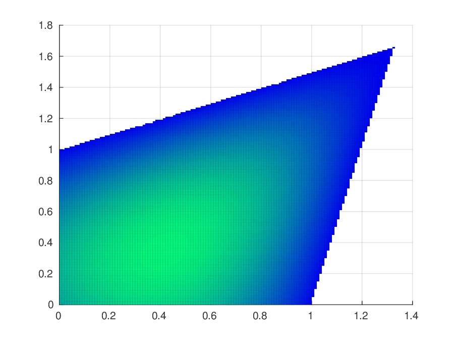 Figure 1
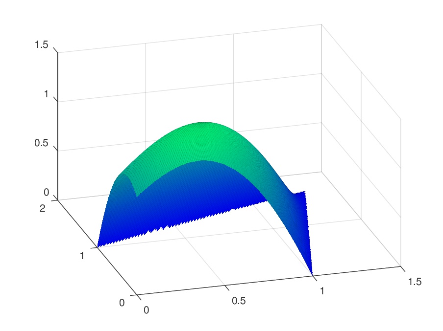 Figure 2
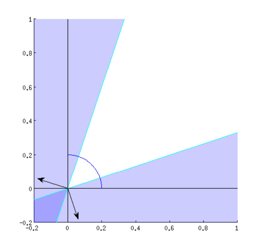 Figure 3
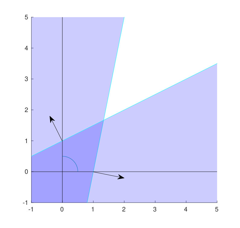 Figure 4
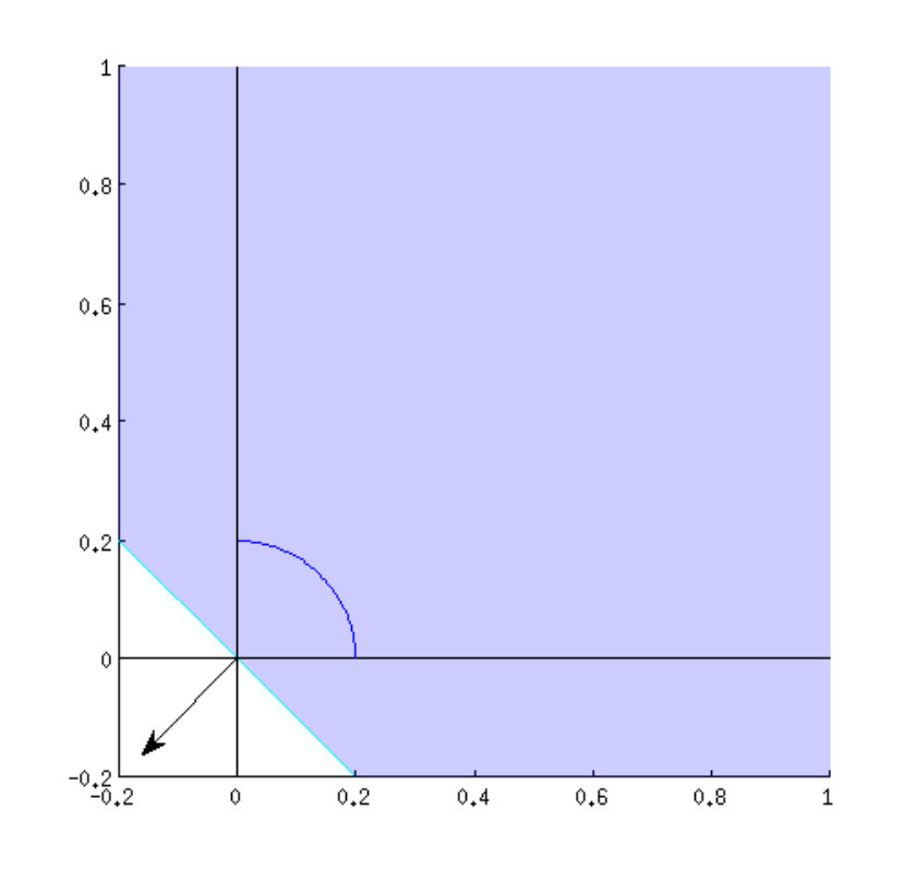 Figure 5
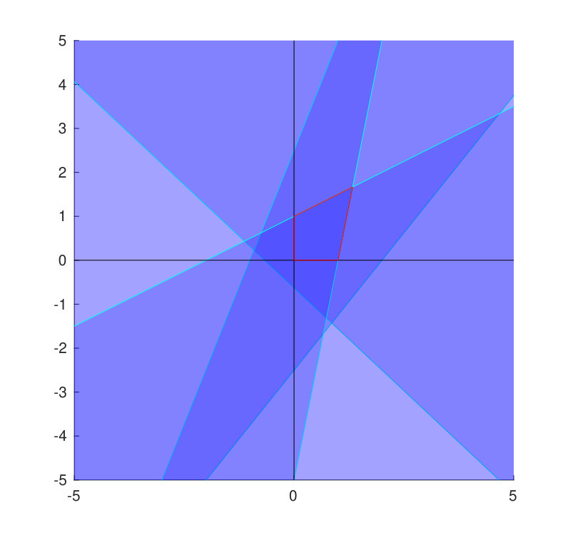 Figure 6
Peer Reviews
No public reviews on file for this paper yet. If you reviewed it on a platform where reviews are public (OpenReview, ICLR, NeurIPS, ICML), you can paste yours below so the community can read it here.
Videos
No videos yet. Explain this paper in a talk, walkthrough, or lecture? Add one.
\addtokomafont
title \addtokomafontsection \addtokomafontsubsection \addtokomafontsubsubsection \addtokomafontparagraph
\NewEnvironLalign
[TABLE]
Existence and Uniqueness for the Multivariate Discrete Terminal Wealth Relative
Andreas Hermes and Stanislaus Maier-Paape
*Institut für Mathematik, RWTH Aachen,
Templergraben 55, D-52062 Aachen, Germany
Abstract In this paper the multivariate fractional trading ansatz of money management from Vince [8] is discussed. In particular, we prove existence and uniqueness of an “optimal ” of the respective optimization problem under reasonable assumptions on the trade return matrix. This result generalizes a similar result for the univariate fractional trading ansatz. Furthermore, our result guarantees that the multivariate optimal solutions can always be found numerically by steepest ascent methods.
Keywords fractional trading, optimal f, multivariate discrete terminal wealth relative, risk and money management, portfolio theory
1 Introduction
Risk and money management for investment issues has always been at the heart of
finance. Going back to the 1950s, Markowitz [7] invented the “modern portfolio theory”,
where the additive expectation of a portfolio of different investments was maximized subject to a given risk expressed by volatility of the portfolio.
When the returns of the portfolio are no longer calculated additive, but multiplicative in order to respect the needs of compound interest, the resulting optimization problem is known as “fixed fractional trading”. In fixed fractional trading strategies an investor always wants to risk a fixed percentage of his current capital for future investments given some distribution of historic trades of his trading strategy.
A first example of factional trading was established in the 1950s by Kelly [2] who found a criterion for an asymptotically optimal investment strategy for one investment instrument. Similarly, Vince in the 1990s (see [8] and [9]) used the fractional trading ansatz to optimize his position sizing. Although at first glance these two methods look quite different, they are in fact closely related as could be shown in [6]. However, only recently in [10], Vince extended the fractional trading ansatz to portfolios of different investment instruments. The situation with investment instruments (systems) and coincident realizations of absolute returns of these systems results in a trade return matrix described in detail in (2.1). Given this trade return matrix, the “Terminal Wealth Relative ” (TWR) can be constructed (see (2.3)) measuring the multiplicative gain of a portfolio resulting from a fixed vector of fractional investments into the systems. In order to find an optimal investment among all fractions the TWR has to be maximized
[TABLE]
where is the definition set of the TWR (see Definition 2.1 and (3.2)).
Whereas in [10], Vince only stated this optimization problem and illustrated it with examples, in Section 3 we give as our main result the necessary analysis. In particular, we investigate the definition set of the TWR and fix reasonable assumptions (Assumption 3.2) under which (1.1) has a unique solution. This unique solution may lie in or on as different examples in Section 4 show. Our result extend the results of Maier–Paape [4], Zhu [12] ( case only) and parts of the PhD of Hermes [1] on the discrete multivariate TWR. One of the main ingredients to show the uniqueness of the maximum of (1.1) is the concavity of the function (see Lemma 3.5). Uniqueness and concavity furthermore guarantee that the solution of (1.1) can always be found numerically by simply following steepest ascent.
Before we start our analysis, some more remarks on related papers are in order.
In [5] Maier–Paape showed that the fractional trading ansatz on one investment instrument leads to tremendous drawdowns, but that effect can be reduced largely when several stochastic independent trading systems are used coincidentally. Under which conditions this diversification effect works out in the here considered multivariate TWR situation is still an open question. Furthermore, several papers investigated risk measures in the context of fractional trading with one investment instrument (; see [3], [4], [6] and [11]). Related investigations for the multivariate TWR using the drawdown can be found in Vince [10].
In the following sections we now analyse the multivariate case of a discrete Terminal Wealth Relative . That means we consider multiple investment strategies where every strategy generates multiple trading returns. As noted before this situation can be seen as a portfolio approach of a discrete Terminal Wealth Relative (cf. [10]). For example one could consider an investment strategy applied to several assets, the strategy producing trading returns on each asset. But in an even broader sense, one could also consider several distinct investment strategies applied to several distinct assets or even classes of assets.
2 Definition of a Terminal Wealth Relative
The subject of consideration in this paper is the multivariate case of the discrete Terminal Wealth Relative for several trading systems analogous to the definition of Ralph Vince in [10]. For we denote the -th trading system by (system k). A trading system is an investment strategy applied to a financial instrument. Each system generates periodic trade returns, e.g. monthly, daily or the like. The absolute trade return of the -th period of the -th system is denoted by , . Thus we have the joint return matrix
[TABLE]
and define
[TABLE]
Just as in the univariate case (cf. [4] or [8]), we assume that each system produced at least one loss within the periods. That means
[TABLE]
Thus we can define the biggest loss of each system as
[TABLE]
For better readability, we define the rows of the given return matrix, i.e. the return of the -th period, as
[TABLE]
and the vector of all biggest losses as
[TABLE]
Having the biggest loses at hand, it is possible to “normalize” the –th column of by such that each system has a maximal loss of . Using the componentwise quotient, the normalized trade matrix return then has the rows
[TABLE]
For , , we define the Holding Period Return (HPR) of the -th period as
[TABLE]
where \langle{\raisebox{-2.15277pt}{\scalebox{1.6}{\cdot}}},{\raisebox{-2.15277pt}{\scalebox{1.6}{\cdot}}}\rangle_{\mathbb{R}^{M}} denotes the standard scalar product on . To shorten the notation, the marking of the vector space at the scalar product is omitted, if the dimension of the vectors is clear. Similar to the univariate case, the gain (or loss) in each system is scaled by its biggest loss. Therefore the represents the gain (loss) of one period, when investing a fraction of of the capital in (system k) for all , thus risking a maximal loss of in the -th trading system.
The Terminal Wealth Relative (TWR) as the gain (or loss) after the given periods, when the fraction is invested in (system k) over all periods, is then given as
[TABLE]
Note that in the –dimensional case a risk of a full loss of our capital corresponds to a fraction of . Here in the multivariate case we have a loss of of our capital every time there exists an such that . That is for example if we risk a maximal loss of in the -th trading system (for some ) and simultaneously letting for all other . However these degenerate vectors of fractions are not the only examples that produce a Terminal Wealth Relative (TWR) of zero. Since we would like to risk at most of our capital (which is quite a meaningful limitation), we restrict to the domain given by the following definition:
Definition 2.1**.**
A vector of fractions is called admissible if holds, where
[TABLE]
Furthermore we define
[TABLE]
With this definition we now have a risk of for each vector of fractions and a risk of less than for each vector of fractions . Since
[TABLE]
we can find an such that
[TABLE]
and thus in particular holds. \|\raisebox{-2.15277pt}{\scalebox{1.6}{\cdot}}\|=\sqrt{\langle{\raisebox{-2.15277pt}{\scalebox{1.6}{\cdot}}},{\raisebox{-2.15277pt}{\scalebox{1.6}{\cdot}}}\rangle} denotes the Euclidean norm on .
Observe that the -th period results in a loss if , that means \langle{(\nicefrac{{\bm{t}_{i\raisebox{-1.07639pt}{\scalebox{1.6}{\cdot}}}}}{{\bm{\hat{t}}}})^{\top}},{\bm{\varphi}}\rangle=\operatorname{HPR}_{i}(\bm{\varphi})-1<0. Hence the biggest loss over all periods for an investment with a given vector of fractions is
[TABLE]
Consequently, we have a biggest loss of
[TABLE]
Note that for we do not have an a priori bound for the fractions , . Thus it may happen that there are with for some (or even for all) , or at least , indicating a risk of more than for the individual trading systems, but the combined risk of all trading systems can still be less than . So the individual risks can potentially be eliminated to some extent through diversification. As a drawback of this favorable effect the optimization in the multivariate case may result in vectors of fractions that require a high capitalization of the individual trading systems. Thus we assume leveraged financial instruments and ignore margin calls or other regulatory issues.
Before we continue with the TWR analysis, let us state a first auxiliary lemma for .
Lemma 2.2**.**
The set in Definition 2.1 is convex, as is .
Proof.
All the conditions and
[TABLE]
define half spaces (which are convex). Since is the intersection of a finite set of half spaces, it is itself convex.
A similar reasoning yields that is convex, too. ∎
3 Optimal Fraction of the Discrete Terminal Wealth Relative
If we develop this line of thought a little further a necessary condition for the return matrix for the optimization of the Terminal Wealth Relative gets clear:
Lemma 3.1**.**
Assume there is a vector with then
[TABLE]
If in addition there is an such that then
[TABLE]
Proof.
If
[TABLE]
it follows that
[TABLE]
For arbitrary the function
[TABLE]
is monotonically increasing in for all and by that we have
[TABLE]
Moreover, if there is an with then
[TABLE]
and by that
[TABLE]
∎
An investment where the holding period returns are greater than or equal to for all periods denotes a “risk free” investment () and considering the possibility of an unbounded leverage, it is clear that the overall profit can be maximized by investing an infinite quantity. Assuming arbitrage free investment instruments, any risk free investment can only be of short duration, hence by increasing the condition will eventually burst, cf. (3.1). Thus, when optimizing the Terminal Wealth Relative , we are interested in settings that fulfill the following assumption
[TABLE]
always yielding .
With that at hand, we can formulate the optimization problem for the multivariate discrete Terminal Wealth Relative
[TABLE]
and analyze the existence and uniqueness of an optimal vector of fractions for the problem under the assumption
Assumption 3.2**.**
*We assume that each of the trading systems in (2.1) produced at least one loss (cf. (2.2)) and furthermore {Lalign} &∀ φ∈∂Bε(0)∩Λε∃ i0=i0(φ)∈{1,…,N}such that ⟨(\nicefrac{{\bm{t}_{i_{0}\raisebox{-1.07639pt}{\scalebox{1.6}{\cdot}}}}}{{\bm{\hat{t}}}})⊤,φ⟩¡0 (no risk free investment)
1N∑i=1Nti,k¿0 ∀ k=1,…,M (each trading system is profitable)
ker(T)={0} (linear independent trading systems)*
Assumption 3.2(3.2) ensures that, no matter how we allocate our portfolio (i.e. no matter what direction we choose), there is always at least one period that realizes a loss, i.e. there exists an with . Or in other words, not only are the investment systems all fraught with risk (cf. (2.2)), but there is also no possible risk free allocation of the systems.
The matrix from (2.1) can be viewed as a linear mapping
[TABLE]
“” denotes the kernel of the matrix in Assumption 3.2(3.2). Thus this assumption is the linear independence of the trading systems, i.e. the linear independence of the columns
[TABLE]
of the matrix . Hence with Assumption 3.2(3.2) it is not possible that there exists an and a such that
[TABLE]
which would make (system ) obsolete. So Assumption 3.2(3.2) is no actual restriction of the optimization problem.
Now we point out a first property of the Terminal Wealth Relative .
Lemma 3.3**.**
Let the return matrix (as in (2.1)) satisfy Assumption 3.2(3.2) then, for all , there exists an such that . In fact .
Proof.
For some arbitrary we have . Then Assumption 3.2(3.2) yields the existence of an with \langle{(\nicefrac{{\bm{t}_{i_{0}\raisebox{-1.07639pt}{\scalebox{1.6}{\cdot}}}}}{{\bm{\hat{t}}}})^{\top}},{\bm{\varphi}}\rangle<0. With
[TABLE]
and
[TABLE]
we get that
[TABLE]
and for all . Hence and clearly (cf. Definition 2.1). ∎
Furthermore the following holds.
Lemma 3.4**.**
Let the return matrix (as in (2.1)) satisfy Assumption 3.2(3.2) then the set is compact.
Proof.
For all Assumption 3.2(3.2) yields an such that \langle{(\nicefrac{{\bm{t}_{i_{0}\raisebox{-1.07639pt}{\scalebox{1.6}{\cdot}}}}}{{\bm{\hat{t}}}})^{\top}},{\bm{\varphi}}\rangle<0. With that we define
[TABLE]
This function is continuous on the compact support . Thus the maximum exists
[TABLE]
Consequently the function
[TABLE]
is well defined and continuous. Since for all
[TABLE]
with equality for at least one index , we have
[TABLE]
and
[TABLE]
hence
[TABLE]
Altogether we see that
[TABLE]
thus the set is bounded and connected as image of the compact set under the continuous function and by that the set is compact. ∎
Now we take a closer look at the third assumption for the optimization problem.
Lemma 3.5**.**
Let the return matrix (as in (2.1)) satisfy Assumption 3.2(3.2) then is concave on . Moreover if there is a with , then is even strictly concave in .
Proof.
For the gradient of is given by the column vector
[TABLE]
where . The Hessian-matrix is then given by
[TABLE]
where \bm{y}_{i}:=\frac{1}{1+\langle{(\nicefrac{{\bm{t}_{i\raisebox{-1.07639pt}{\scalebox{1.6}{\cdot}}}}}{{\bm{\hat{t}}}})^{\top}},{\bm{\varphi}}\rangle}(\nicefrac{{\bm{t}_{i\raisebox{-1.07639pt}{\scalebox{1.6}{\cdot}}}}}{{\bm{\hat{t}}}})\in\mathbb{R}^{1\times M} is a row vector. The matrix can be rearranged as
[TABLE]
Since the matrices are positive semi-definite for all , the same holds for and therefore is concave. Furthermore if there is a with
[TABLE]
where , the matrix further reduces to
[TABLE]
If is not strictly positive definite there is a such that
[TABLE]
and we get that
[TABLE]
yielding a non trivial element in and thus contradicting Assumption 3.2(3.2). Hence matrix is strictly positive definite and is strictly concave in . ∎
With this at hand we can state an existence and uniqueness result for the multivariate optimization problem.
Theorem 3.6**.**
(optimal existence) Given a return matrix T=\bigg{(}t_{i,k}\bigg{)}_{\begin{subarray}{c}1\leq i\leq N\\ 1\leq k\leq M\end{subarray}} as in (2.1) that fulfills Assumption 3.2, then there exists a solution of the optimization problem (3.2)
[TABLE]
Furthermore one of the following statements holds:
- (a)
* is unique, or* 2. (b)
*. *
For both cases , and hold true.
Proof.
We show existence and partly uniqueness of a maximum of the -th root of , yielding existence and partly uniqueness of a solution of (3.4) with the claimed properties.
With Lemma 2.2 and Lemma 3.4, the support of the Terminal Wealth Relative is convex and compact. Hence the continuous function attains its maximum on . For we get from (3.3)
[TABLE]
which is a vector whose components are strictly positive due to Assumption 3.2(3.2). Therefore is not a maximum of and a global maximum reaches a value greater than
[TABLE]
Since for all
[TABLE]
holds, a maximum can not be attained in either.
Now if there is a maximum on , assertion (b) holds together with the claimed properties. Alternatively, a maximum is attained in the interior . In this case, Lemma 3.5 yields the strict concavity of at . Suppose there is another maximum then the straight line connecting both maxima
[TABLE]
is fully contained in the convex set (cf. Lemma 2.2). Because of the concavity of all points of have to be maxima, which is a contradiction to the strict concavity of in . Thus the maximum is unique and assertion (a) holds together with the claimed properties. ∎
In the remaining of this section, we will further discuss case (b) in Theorem 3.6. We aim to show that the maximum is unique either, but we proof this using a completely different idea. In order to lay the grounds for this, first, we give a lemma:
Lemma 3.7**.**
If from (2.1) is a return map satisfying Assumption 3.2 and if , then each return map , which results from after eliminating one of its columns, is also a return map satisfying Assumption 3.2.
Proof.
Since each of the trading systems of the return matrix has a biggest loss , , the same holds for the trading systems of the reduced matrix .
For , Assumption 3.2 (3.2) and (3.2) follow straight from the respective properties of the matrix .
Now let, without loss of generality, be the matrix that results from by eliminating the last column, i.e. the -th trading system is omitted. Let \bm{t}_{i\raisebox{-1.50694pt}{\scalebox{1.6}{\cdot}}}^{(M-1)}\in\mathbb{R}^{M-1}, , denote the rows of and the vector of biggest losses of . Then for Assumption 3.2 (3.2) we have to show that
[TABLE]
such that
[TABLE]
Using Assumption 3.2 (3.2) for matrix and
[TABLE]
the inequality
[TABLE]
holds true. Thus (3.5) holds likewise. ∎
Having this at hand, we can now extend Theorem 3.6.
Corollary 3.8**.**
(optimal uniqueness) In the situation of Theorem 3.6 the uniqueness also holds for case (b), i.e. a maximum is also a unique maximum of in .
Proof.
Assume that the optimal solution is not unique, then there exists an additional optimal solution with . Since is convex (c.f. Lemma 2.2), the line connecting both solutions
[TABLE]
is fully contained in . Because of the concavity of on (c.f. Lemma 3.5), all points on are optimal solutions. Therefore must be a subset of , since we have seen that an optimal solution in the interior would be unique. Hence, there is (at least) one such that, for all investment vectors in , the trading system (system ) is not invested . I.e. the -th component of , and all vectors in is zero.
Without loss of generality, let . Then
[TABLE]
are two optimal solutions for
[TABLE]
But with that, the -dimensional investment vectors and are two distinct optimal solutions for
[TABLE]
With Lemma 3.7 the return map , which results from after eliminating the -th column (i.e. (system )) satisfies Assumption 3.2. Applying Theorem 3.6 to the sub-dimensional optimization problem, yields that and again lie at the boundary of the admissible set of investment vectors .
Hence, we have two distinct optimal solutions on the boundary for the optimization problem with investment systems. By induction this reasoning leads to the existence of two distinct optimal solutions for an optimization problem with just one single trading system. But for that type of problem, we already know that the solution is unique (see for example [4]), which causes a contradiction to our assumption. Thus, also for case (b) we have the uniqueness of the solution . ∎
Remark 3.9**.**
Note that Assumption 3.2(3.2) is necessary for uniqueness. To give a counterexample imagine a return matrix with two equal columns, meaning the same trading system is used twice. Let be the optimal f for this one dimensional trading system. Then it is easy to see that , and the straight line connecting these two points yield TWR optimal solutions for the return matrix .
4 Example
As an example we fix the joint return matrix for trading systems and the returns from periods given through the following table.
[TABLE]
Obviously every system produced at least one loss within the periods, thus the vector with
[TABLE]
is well-defined. For the takes the form
[TABLE]
where the set of admissible vectors is given by
[TABLE]
Since for all
[TABLE]
we have
[TABLE]
Accordingly we get
[TABLE]
When examining the -th row \bm{t}_{6\raisebox{-1.50694pt}{\scalebox{1.6}{\cdot}}}=(-1,-1,-1,-1) of the matrix we observe that Assumption 3.2(3.2) is fulfilled with . To see that let, for some , , then
[TABLE]
For Assumption 3.2(3.2) one can easily check that all four systems are “profitable”, since the mean values of all four columns in (4.8) are strictly positive. Lastly, for Assumption 3.2(3.2) we check that the rows of matrix are linearly independent
[TABLE]
Thus Theorem 3.6 yields the existence and uniqueness of an optimal investment fraction with , and , which can numerically be computed
[TABLE]
In the above example, a crucial point is that there is one row in the return matrix where the -th entry is the biggest loss of (system k), . Such a row in the return matrix implies, that all trading systems realized their biggest loss simultaneously, which can be seen as a strong evidence against a sufficient diversification of the systems. Hence we analyze Assumption 3.2(3.2) a little closer to see what happens if this is not the case.
With the help of Assumption 3.2(3.2), for all , there is a row of the return matrix \bm{t}_{i_{0}\raisebox{-1.50694pt}{\scalebox{1.6}{\cdot}}}, such that \langle{(\nicefrac{{\bm{t}_{i_{0}\raisebox{-1.07639pt}{\scalebox{1.6}{\cdot}}}}}{{\bm{\hat{t}}}})^{\top}},{\bm{\varphi}}\rangle<0. The sets
[TABLE]
describe the hyperplanes generated by the normal direction (\nicefrac{{\bm{t}_{i\raisebox{-1.07639pt}{\scalebox{1.6}{\cdot}}}}}{{\bm{\hat{t}}}})^{\top}\in\mathbb{R}^{M}, . Thus each from the set has to be an element of one of the half spaces
[TABLE]
In other words the set has to be a subset of a union of half spaces
[TABLE]
If there exists an index such that for all , then the normal direction of the corresponding hyperplane is
[TABLE]
hence
[TABLE]
and therefore Assumption 3.2(3.2) is fulfilled. Figure 1 shows a hyperplane for and a row of the return matrix where all entries are the biggest losses, that means the normal direction of this hyperplane is the vector
[TABLE]
However, it is not necessary for Assumption 3.2(3.2) that the set is covered by just one hyperplane. Again for an illustration of possible hyperplanes can be seen in Figure 2. The figure on the left shows a case where Assumption 3.2(3.2) is violated and the figure on the right a case where it is satisfied.
For the next example we fix the return matrix as
[TABLE]
with and . Thus the biggest losses of the two systems are
[TABLE]
To determine the set of admissible investments (and to check Assumption 3.2) we examine the vectors (\nicefrac{{\bm{t}_{i\raisebox{-1.07639pt}{\scalebox{1.6}{\cdot}}}}}{{\bm{\hat{t}}}}) for
[TABLE]
and solve the linear equations
[TABLE]
The solutions for are shown in Figure 3.
Each solution corresponds to a “cyan” line. The area where the inequality \langle{(\nicefrac{{\bm{t}_{i\raisebox{-1.07639pt}{\scalebox{1.6}{\cdot}}}}}{{\bm{\hat{t}}}})^{\top}},{\bm{\varphi}}\rangle\geq-1 holds for some is shaded in “light blue”. The set where the inequalities hold for all is the section where all shaded areas overlap, thus the “dark blue” section. Therefore the set of admissible investments is given by
[TABLE]
with
[TABLE]
Assumption 3.2 is fulfilled, since
- (a)
the half spaces for rows and of the return matrix cover the whole set (cf. Figure 2 b), 2. (b)
and and 3. (c)
obviously, the columns of the return matrix are linearly independent.
A plot of the Terminal Wealth Relative for the return matrix from (4.9) can be seen in Figure 4 and 5 with a maximum at
[TABLE]
Therefore the maximum is clearly attained in the interior .
The following example will show that the unique maximum of Theorem 3.6 can indeed be attained on , i.e. the case discussed in Corollary 3.8. For that we add a third investment system to our last example (4.10) with the new returns
[TABLE]
such that the vectors (\nicefrac{{\bm{t}_{i\raisebox{-1.07639pt}{\scalebox{1.6}{\cdot}}}}}{{\bm{\hat{t}}}}), , form the matrix
[TABLE]
This set of trading systems fulfills Assumption 3.2(3.2) since .
Assumption 3.2(3.2) is satisfied as well, because the three columns of are linearly independent. For Assumption 3.2(3.2) we have to show that
[TABLE]
holds. If not, we would have an investment vector
[TABLE]
such that (4.14) is not true for all rows of the matrix . In particular if we look at lines 4 and 5
[TABLE]
the sum of both inequalities still has to be true
[TABLE]
which is a contradiction to being an element of .
Now we examine the following vector of investments
[TABLE]
with the unique maximum of the optimization problem of the reduced set of trading systems from the last example (cf. (4.12)).
The first derivative of the Terminal Wealth Relative in the direction of the third component at is given by
[TABLE]
Moreover with being the optimal solution of the last example in two variables we have
[TABLE]
Thus is indeed a local maximal point on the boundary of for with the three trading systems in (4.13). Corollary 3.8 yields the uniqueness of this maximal solution for
[TABLE]
5 Conclusion
With our main theorems, Theorem 3.6 and Corollary 3.8, we were able give a complete existence and uniqueness theory for the optimization problem (3.2) of a multivariate Terminal Wealth Relative under reasonable assumptions. Furthermore, due to the convexity of the domain (Lemma 2.2), the concavity of (see Lemma 3.5) and the uniqueness of the “optimal ” solution, it is always guaranteed that simple numerical methods like steepest ascent will find the maximum.
The reference list from the paper itself. Each links out to its DOI / PubMed record.
- 1[1] Andreas Hermes, A mathematical approach to fractional trading, Ph D–thesis, Institut für Mathematik, RWTH Aachen, (2016).
- 2[2] J. L. Kelly, Jr. A new interpretation of information rate, Bell System Technical J. 35:917-926, (1956).
- 3[3] Marcos Lopez de Prado, Ralph Vince and Qiji Jim Zhu, Optimal risk budgeting under a finite investment horizon, Availabe at SSRN 2364092, (2013).
- 4[4] Stanislaus Maier–Paape, Existence theorems for optimal fractional trading, Institut für Mathematik, RWTH Aachen, Report Nr. 67 (2013).
- 5[5] Stanislaus Maier–Paape, Optimal 𝐟 𝐟 f and diversification, International Federation of Technical Analysis Journal, 15:4-7, (2015).
- 6[6] Stanislaus Maier–Paape, Risk averse fractional trading using the current drawdown, Institut für Mathematik, RWTH Aachen, Report Nr. 88 (2016).
- 7[7] Henry M. Markowitz, Portfolio Selection, Finanz Buch Verlag, (1991).
- 8[8] Ralph Vince, Portfolio Management Formulas: Mathematical Trading Methods for the Futures, Options, and Stock Markets, John Wiley & Sons, Inc., (1990).