Heat generation with plasmonic nanoparticles
Habib Ammari, Francisco Romero, Matias Ruiz

TL;DR
This paper analyzes heat generation by plasmonic nanoparticles of arbitrary shapes under resonance illumination, revealing significant temperature deviations in close-to-touching particles, with implications for biomedical detection and thermal monitoring.
Contribution
It introduces a mathematical framework using layer potentials and asymptotic analysis for arbitrary-shaped nanoparticles, including multiple particles, at plasmonic resonance.
Findings
Temperature fields differ significantly for close-to-touching nanoparticles.
The analysis enables better detection of nanoparticles in biological media.
It provides insights into temperature elevation in tissue due to nanoparticle heating.
Abstract
In this paper we use layer potentials and asymptotic analysis techniques to analyze the heat generation due to nanoparticles when illuminated at their plasmonic resonance. We consider arbitrary-shaped particles and both single and multiple particles. For close-to-touching nanoparticles, we show that the temperature field deviates significantly from the one generated by a single nanoparticle. The results of this paper open a door for solving the challenging problems of detecting plasmonic nanoparticles in biological media and monitoring temperature elevation in tissue generated by nanoparticle heating.
Click any figure to enlarge with its caption.
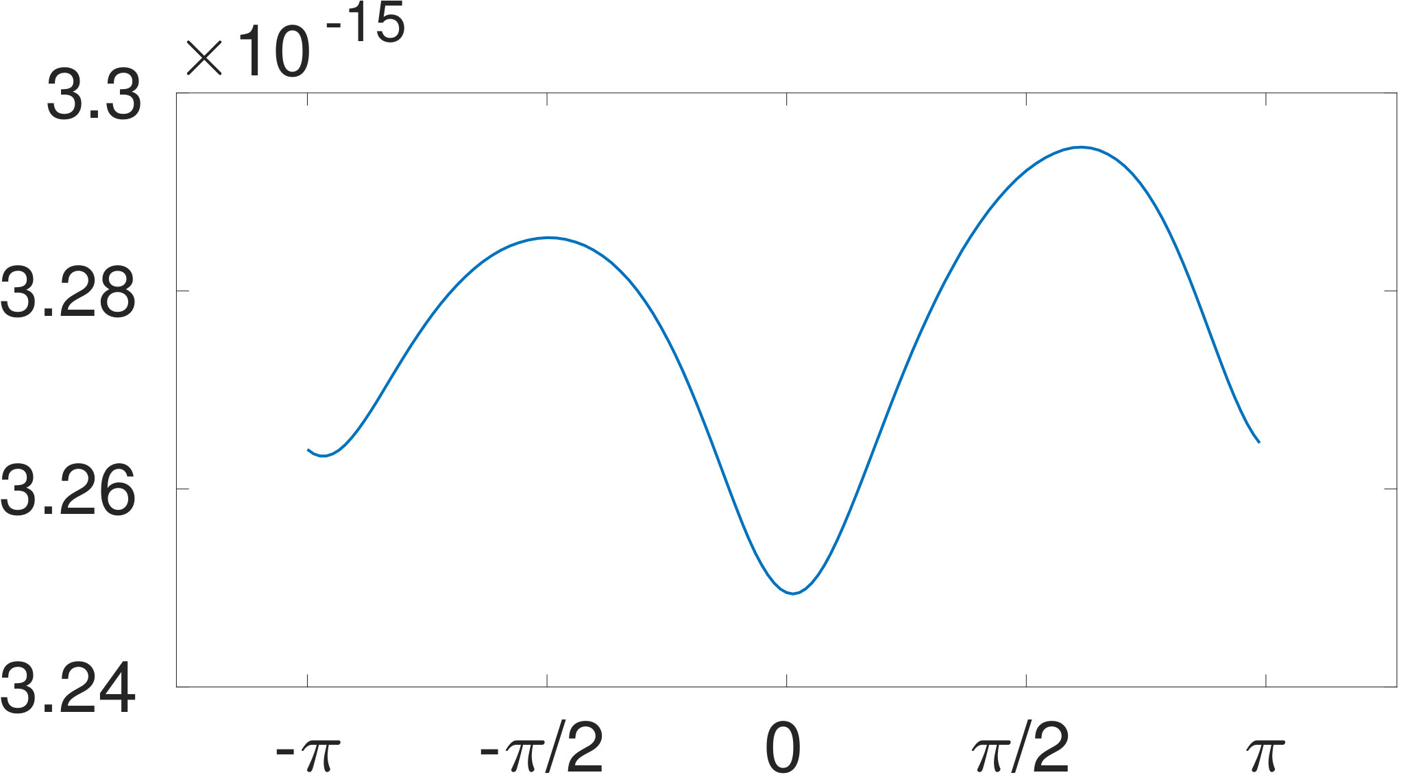 Figure 1
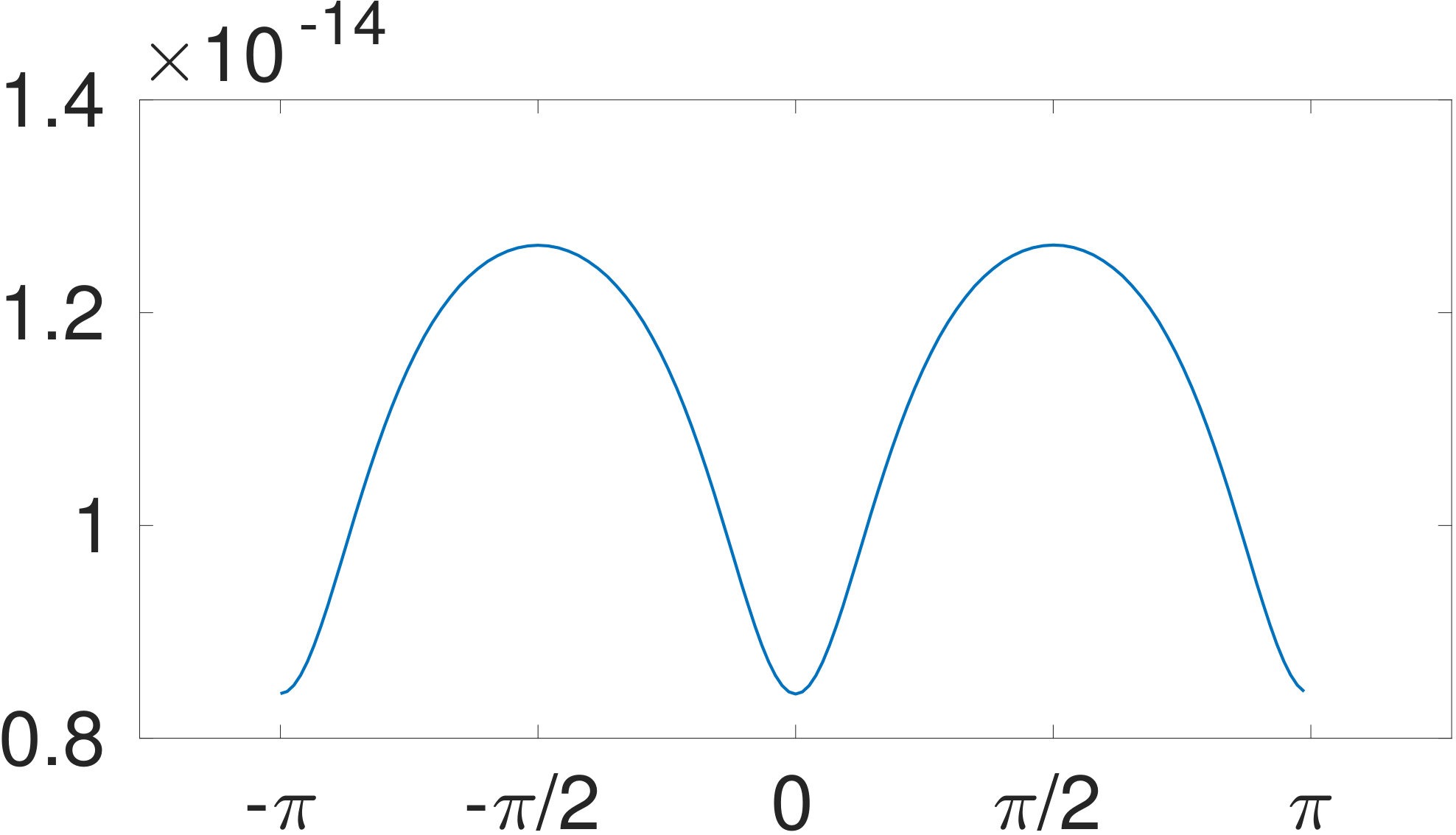 Figure 1
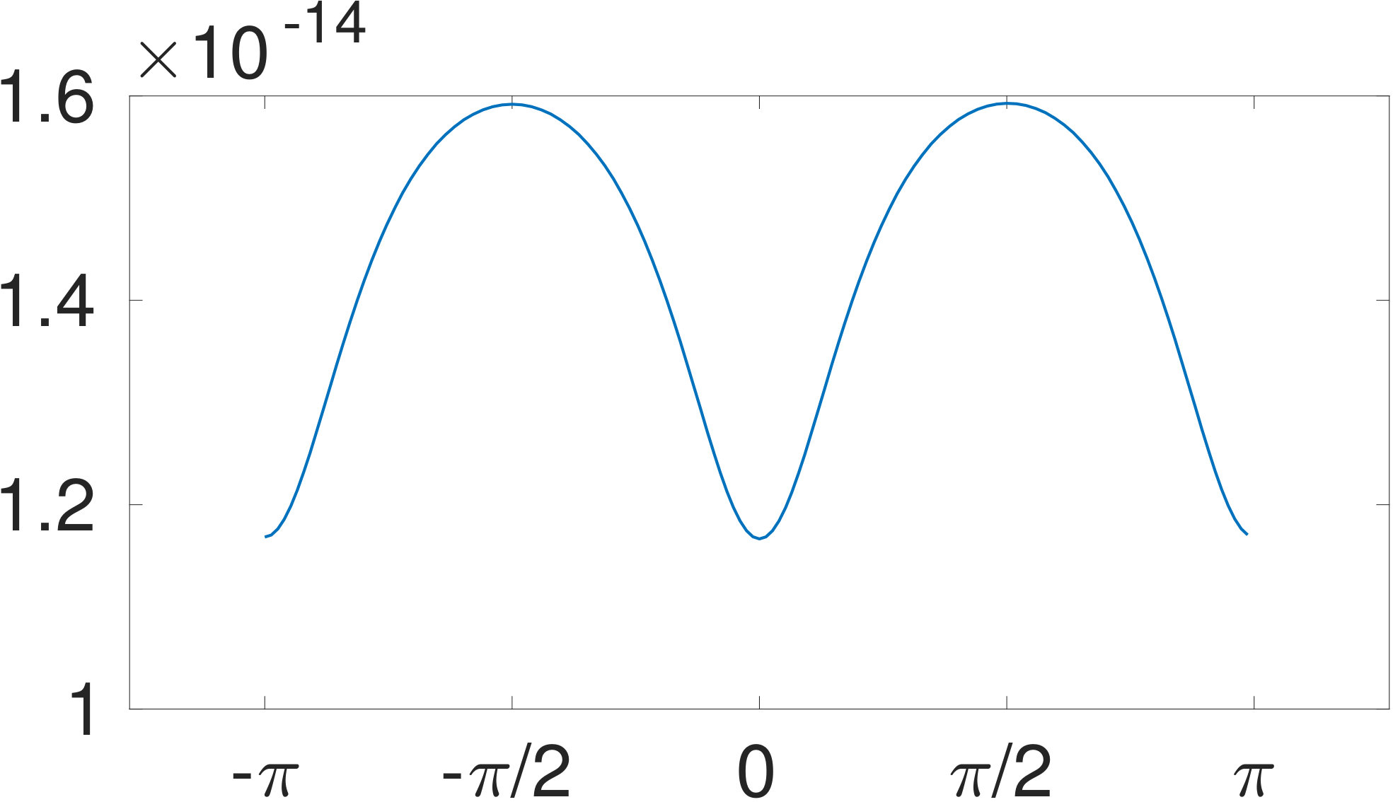 Figure 1
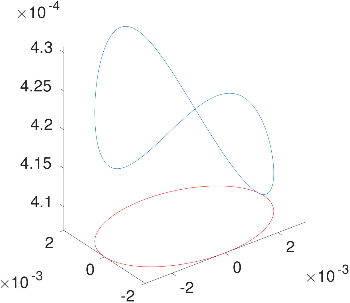 Figure 1
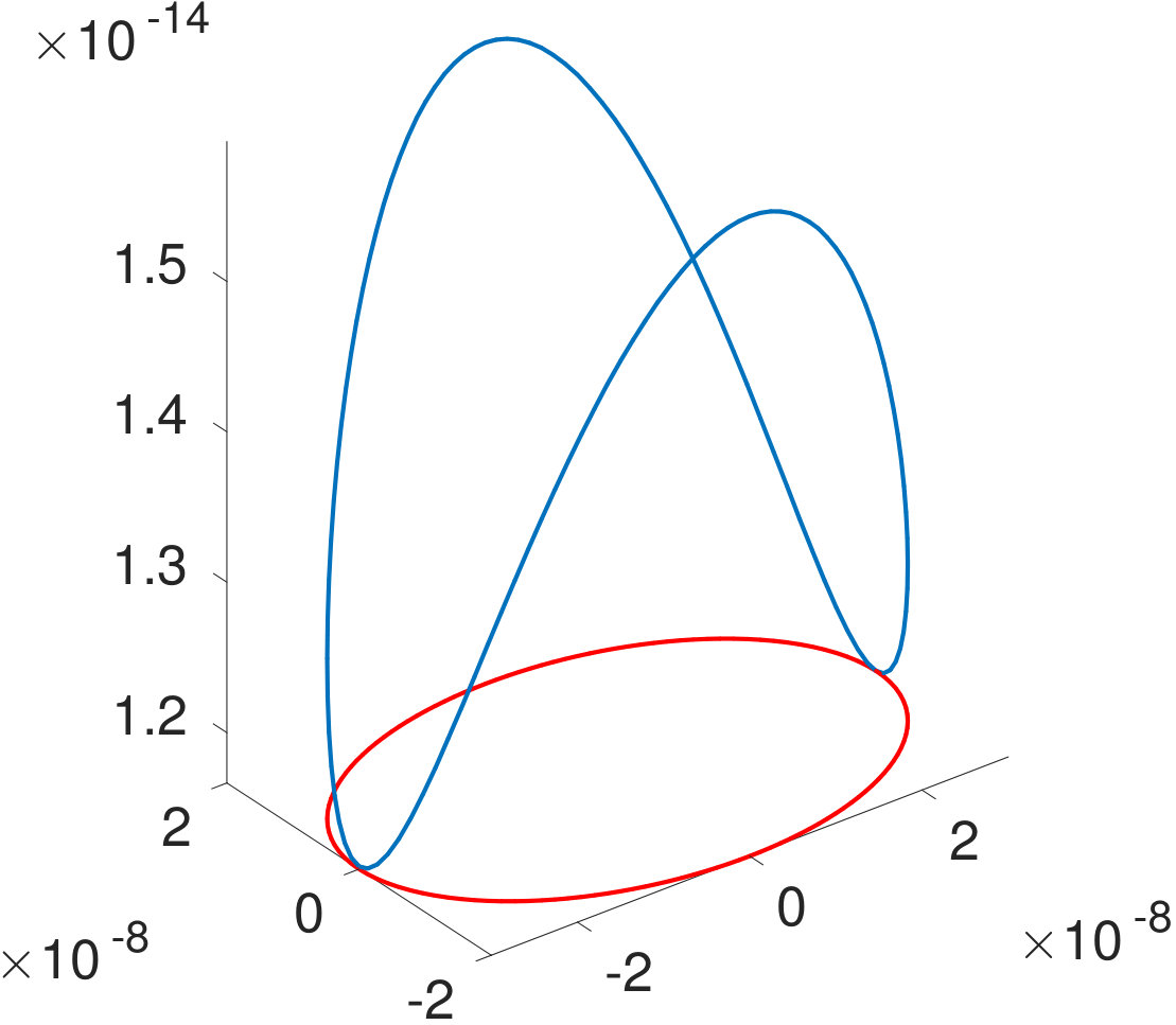 Figure 1
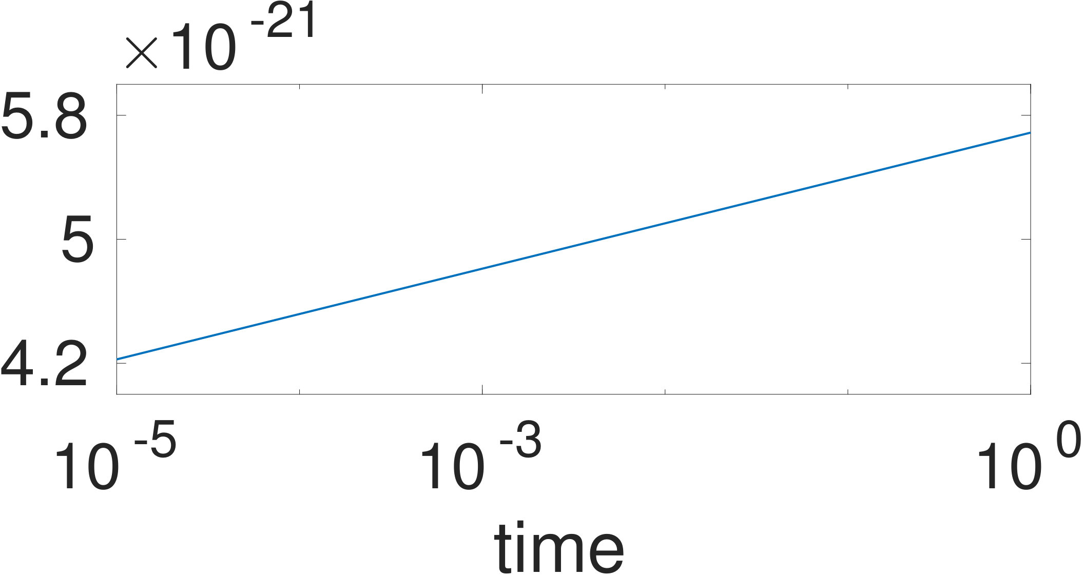 Figure 1
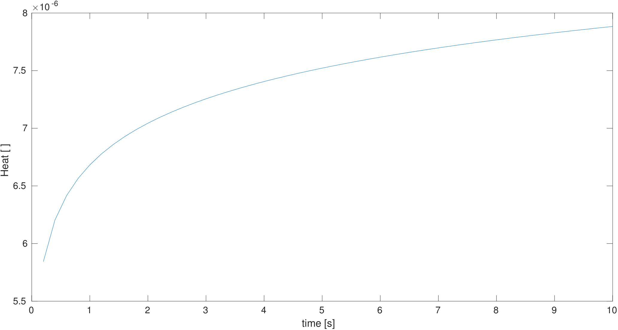 Figure 1
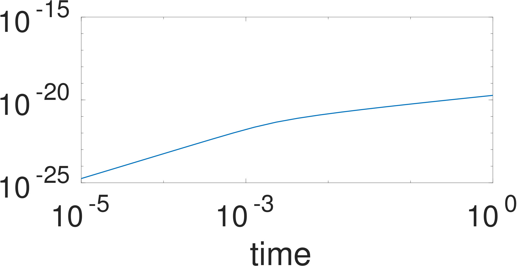 Figure 1
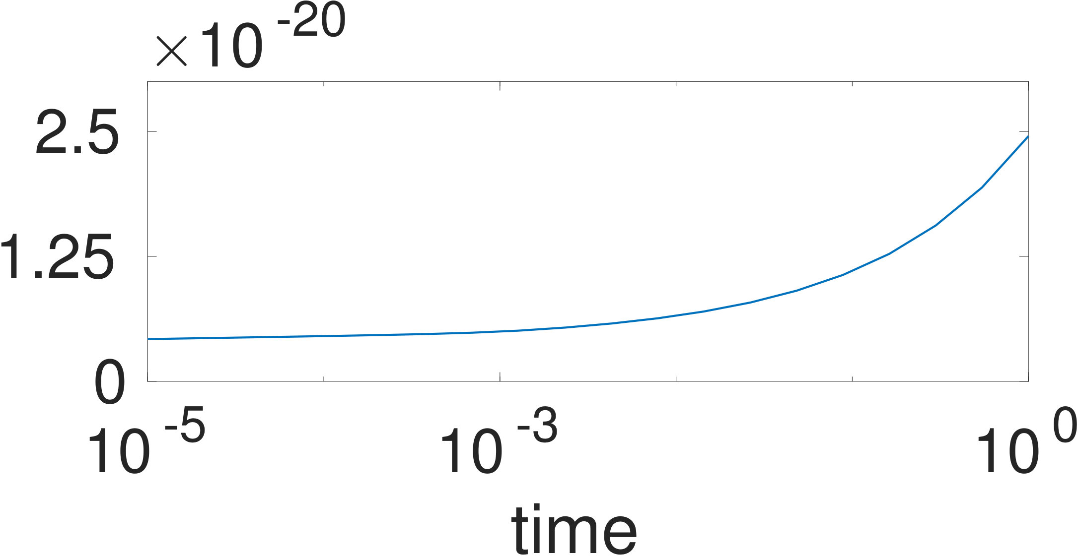 Figure 1
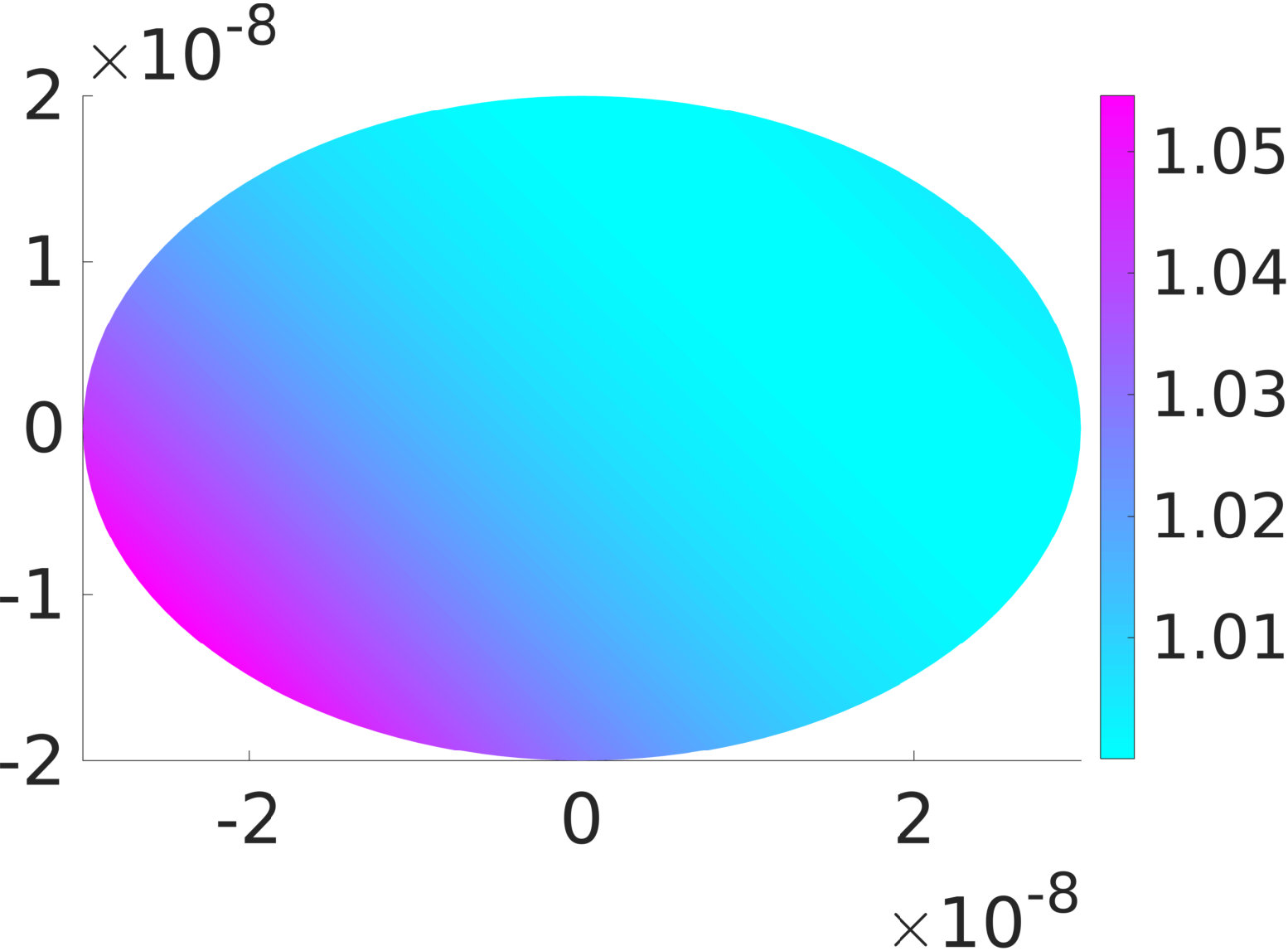 Figure 1
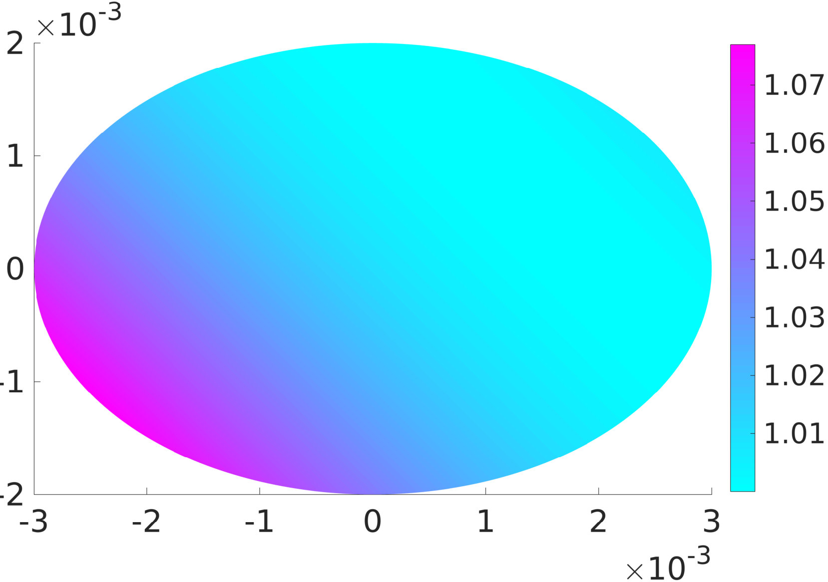 Figure 1
 Figure 1
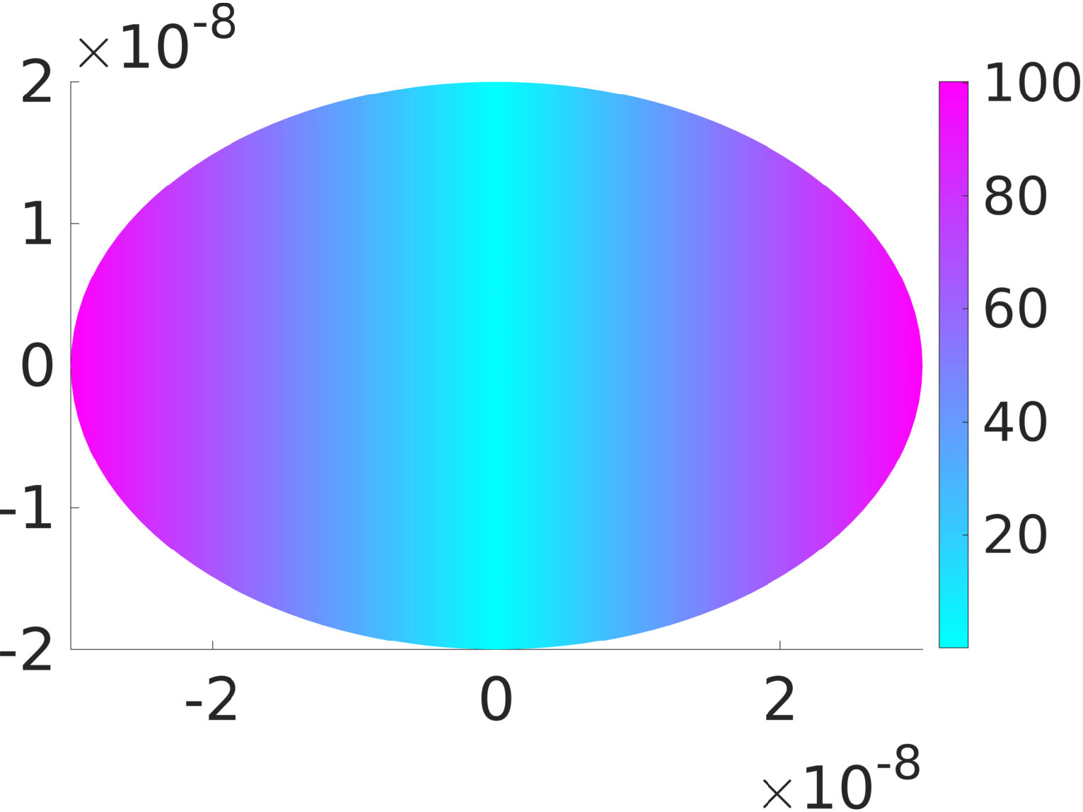 Figure 1
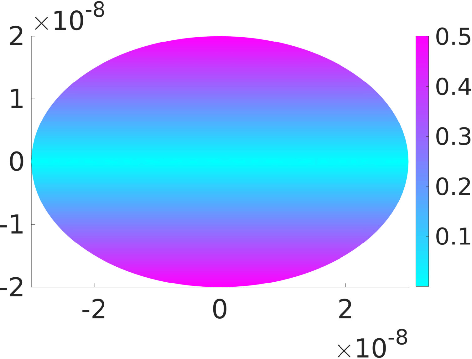 Figure 1
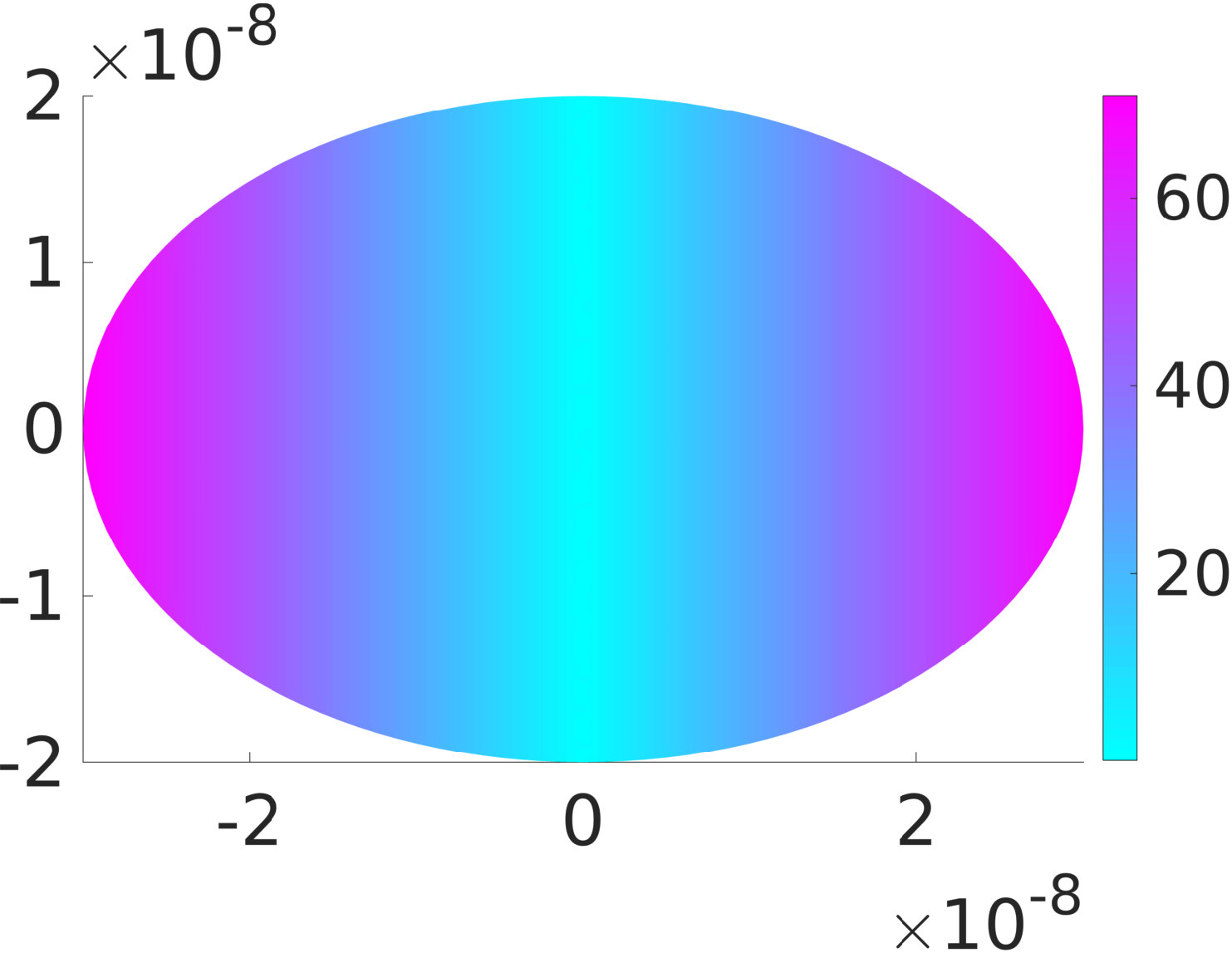 Figure 1
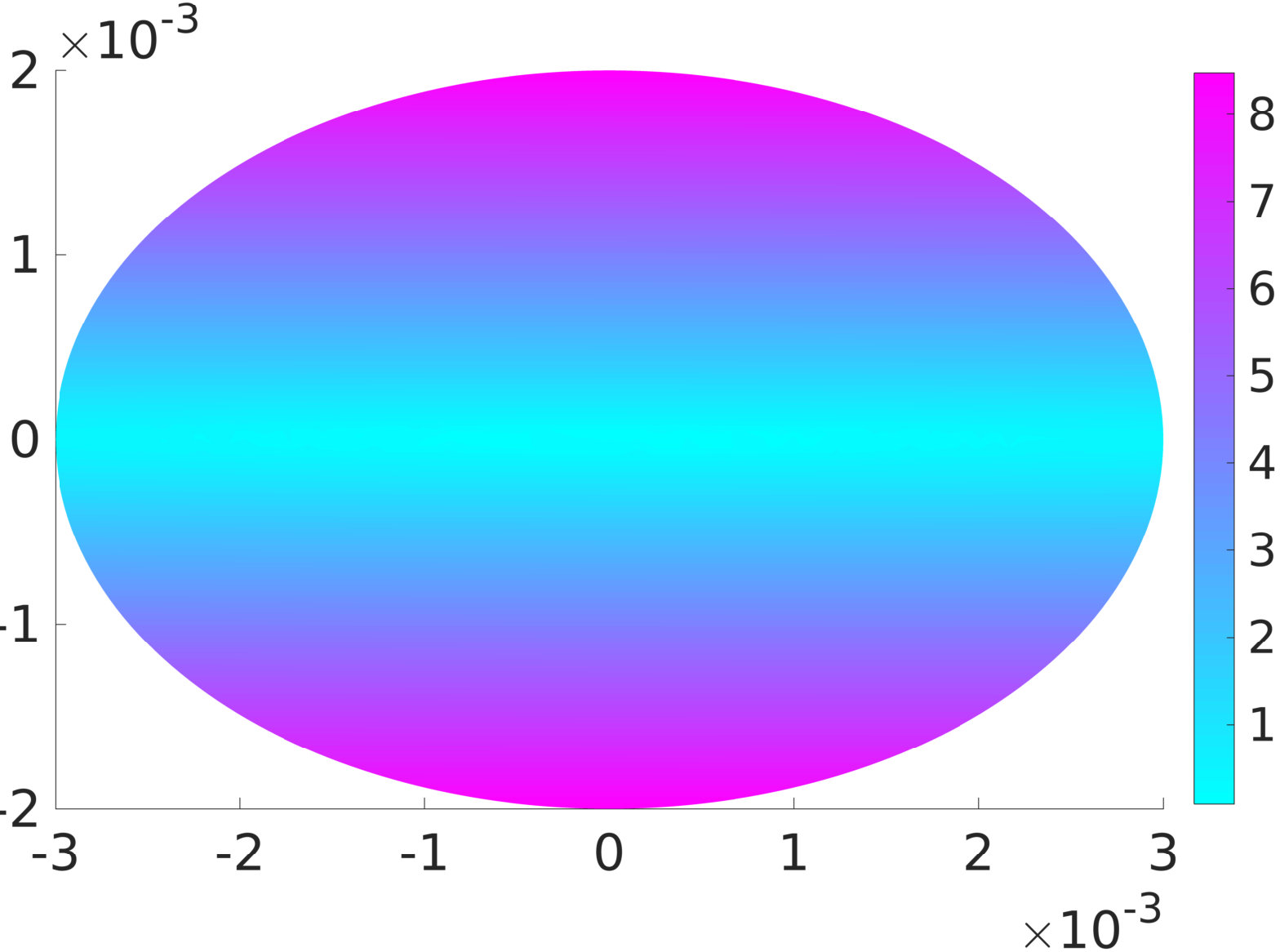 Figure 1
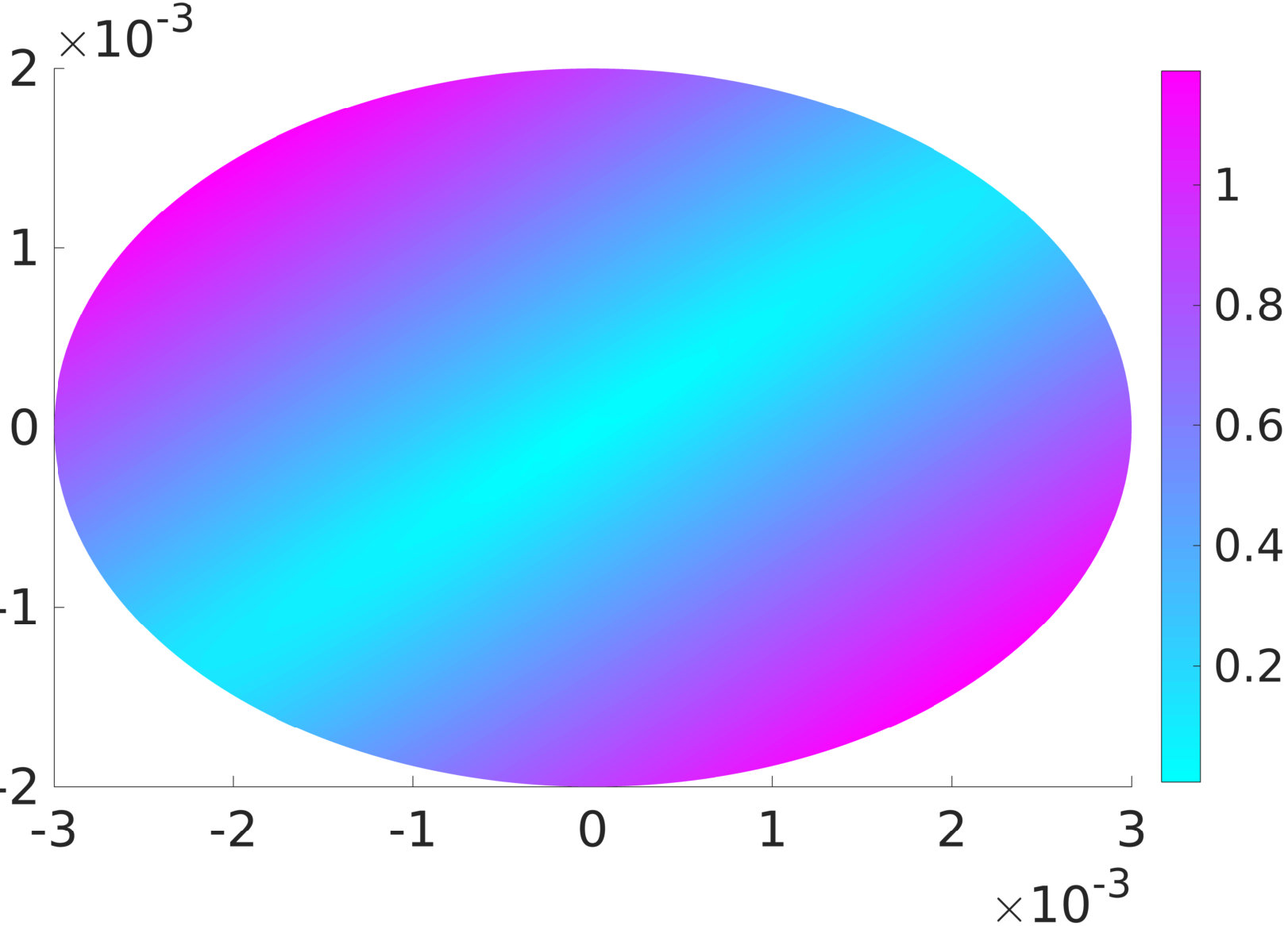 Figure 1
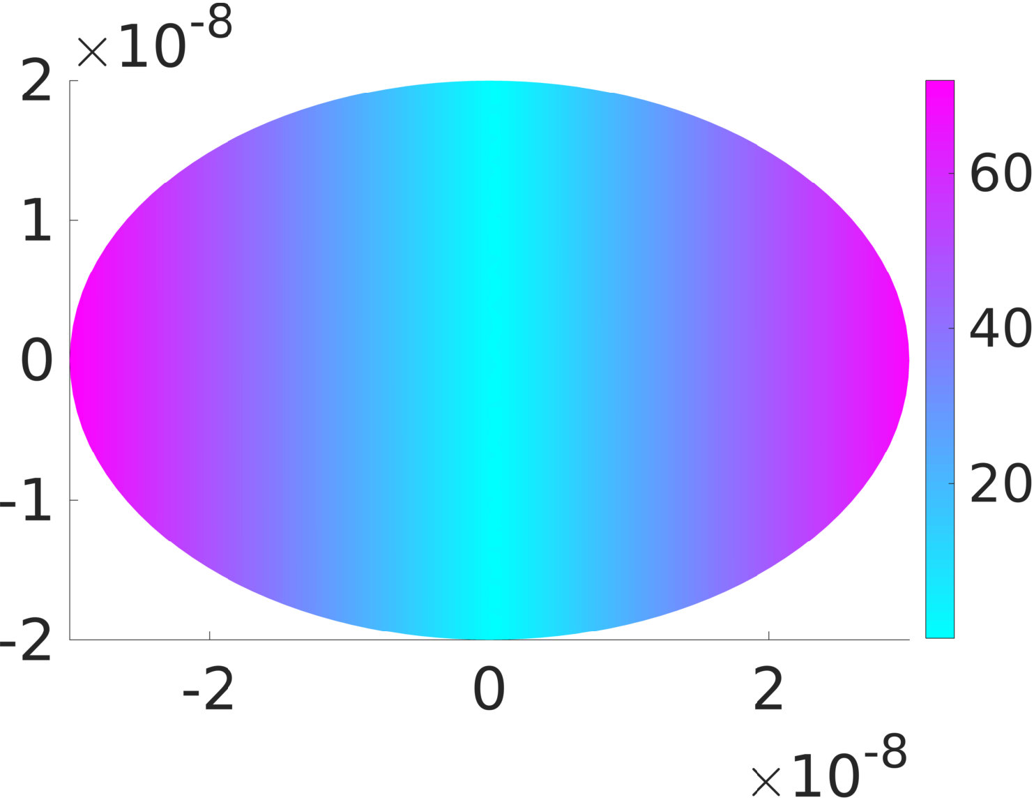 Figure 1
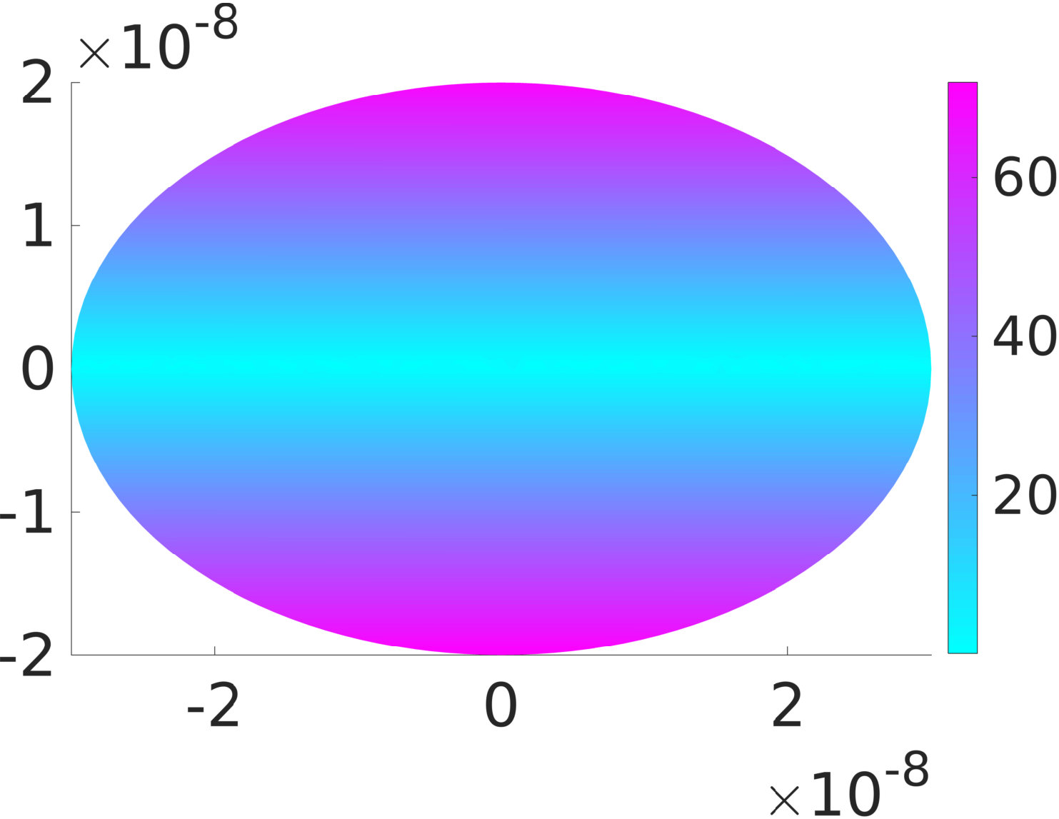 Figure 1
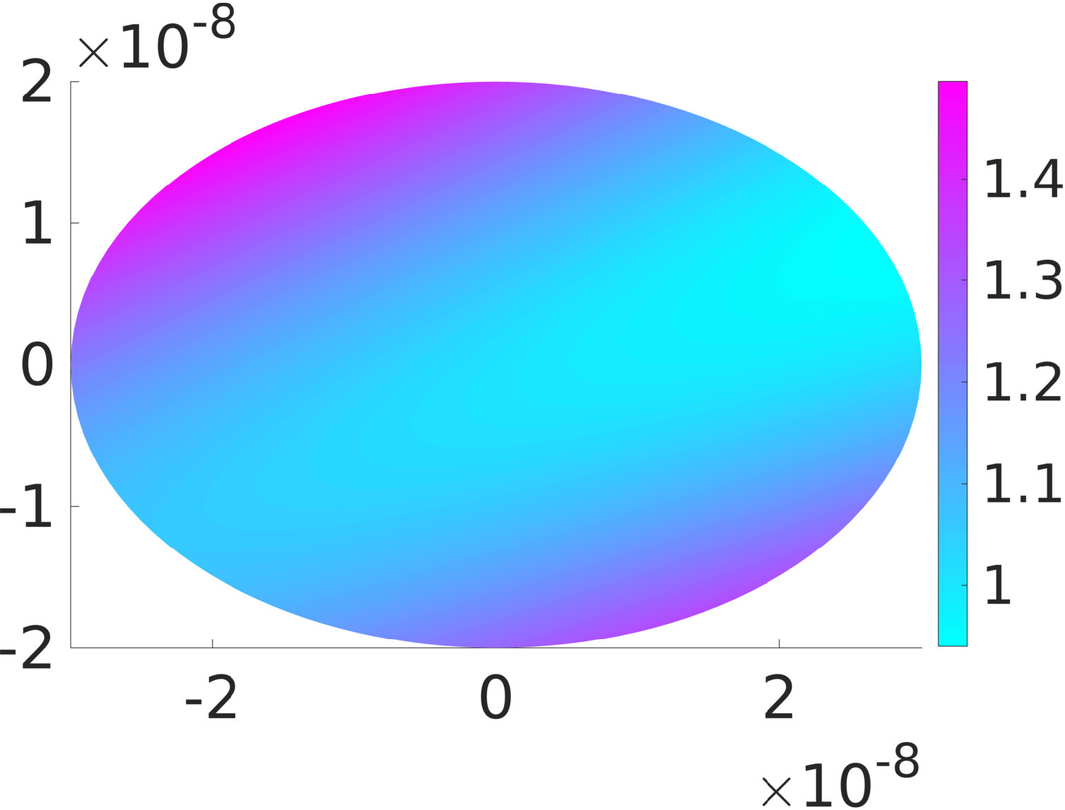 Figure 1
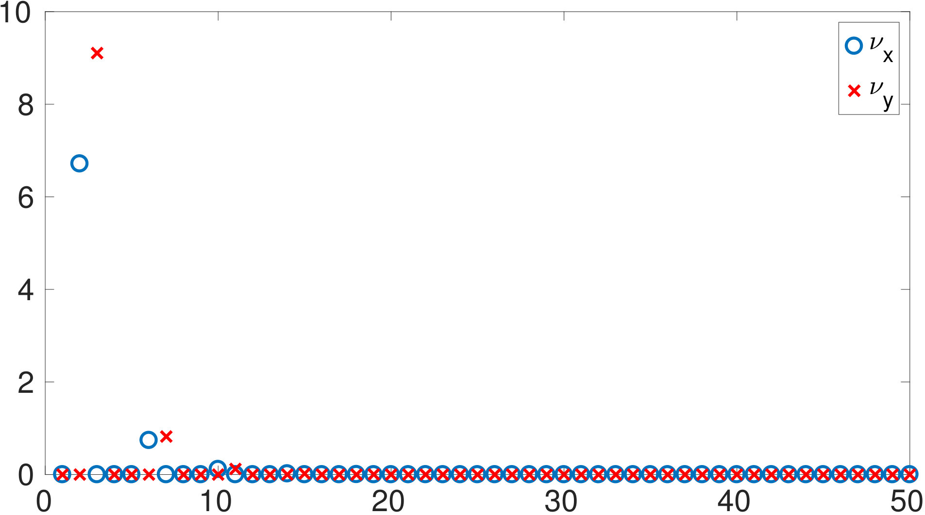 Figure 1
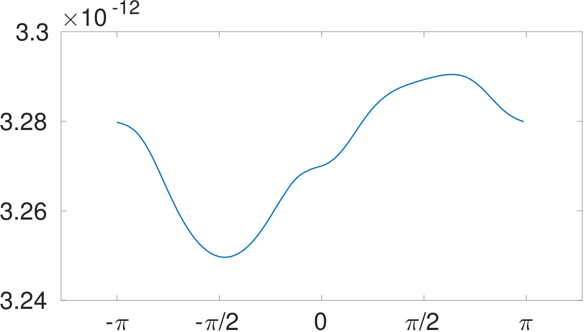 Figure 2
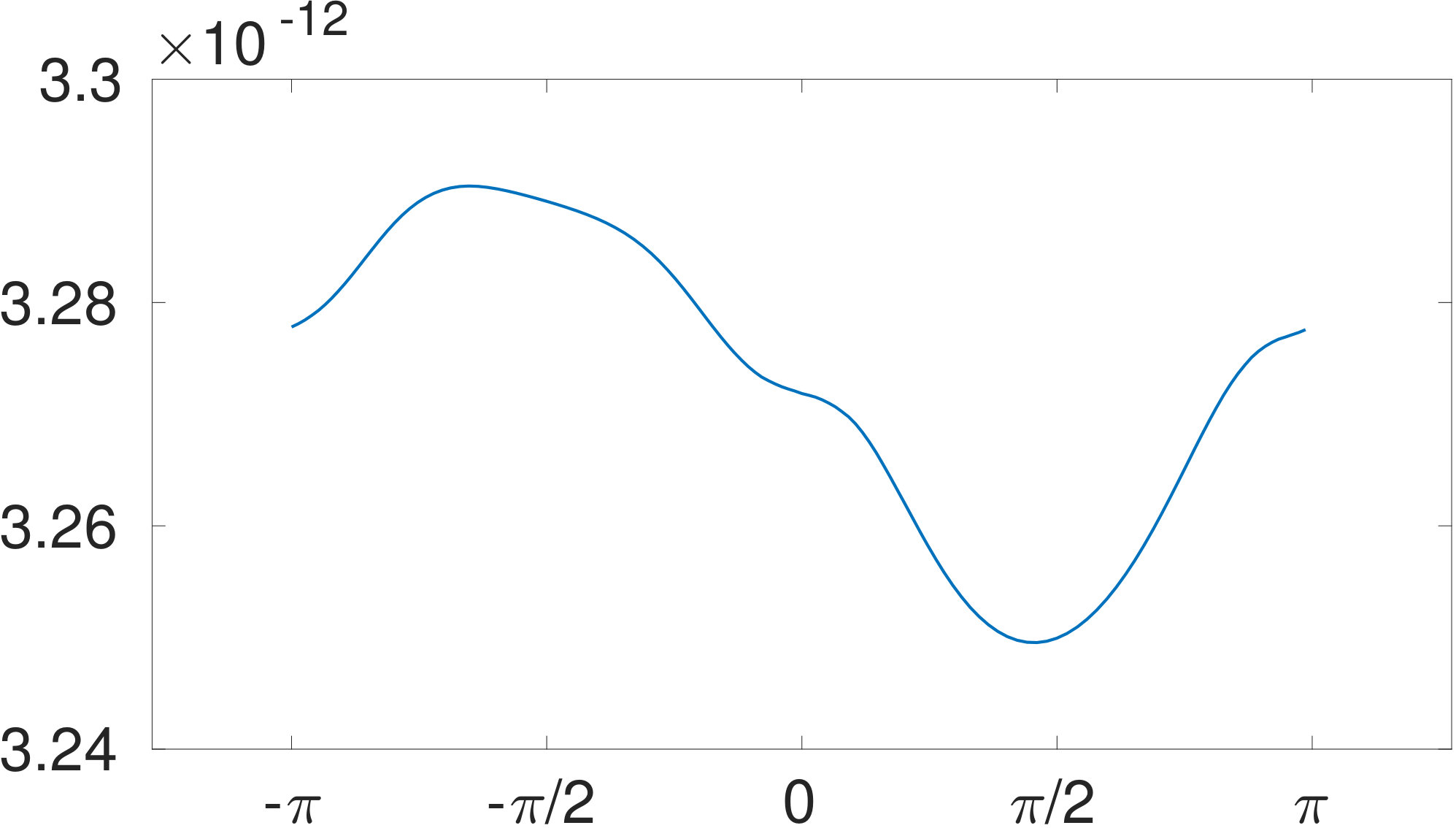 Figure 2
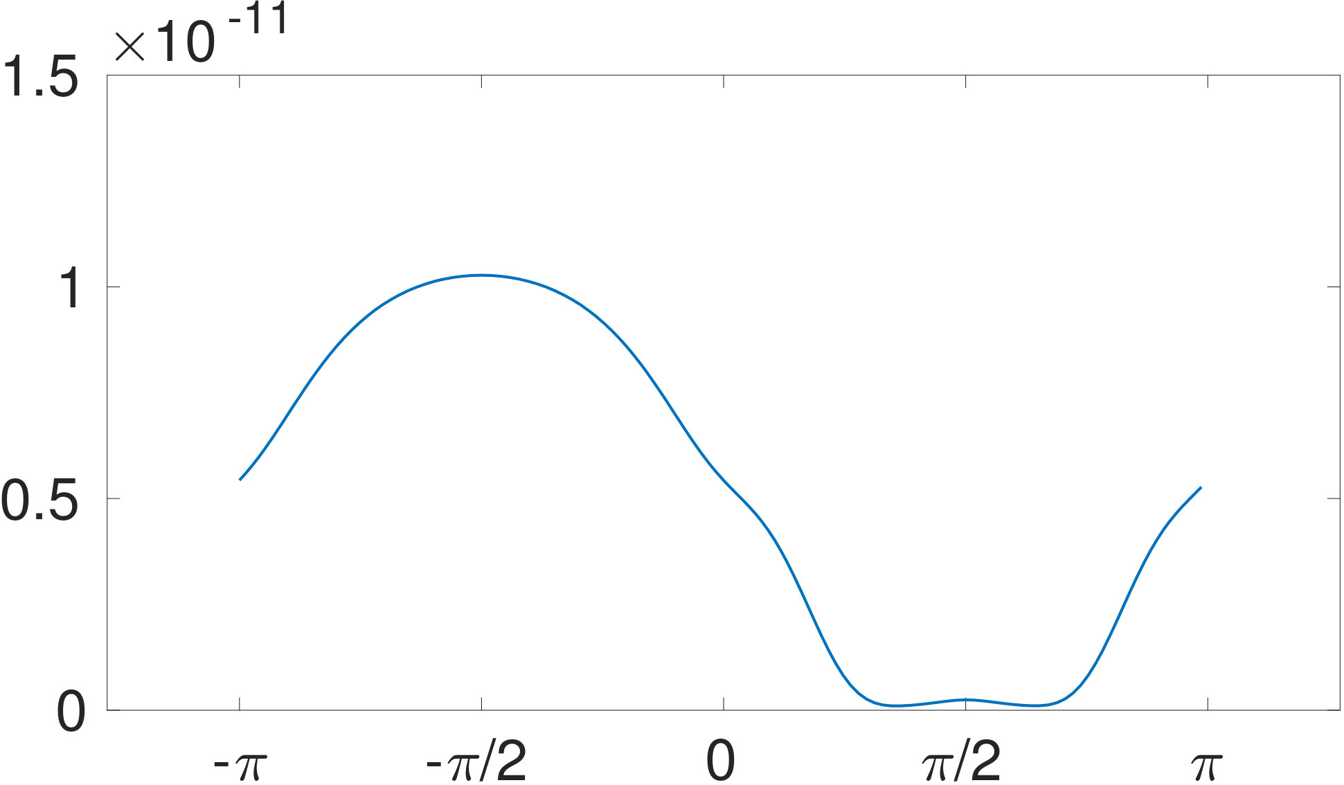 Figure 2
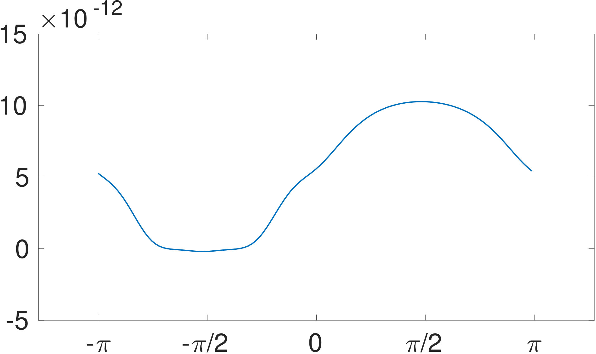 Figure 2
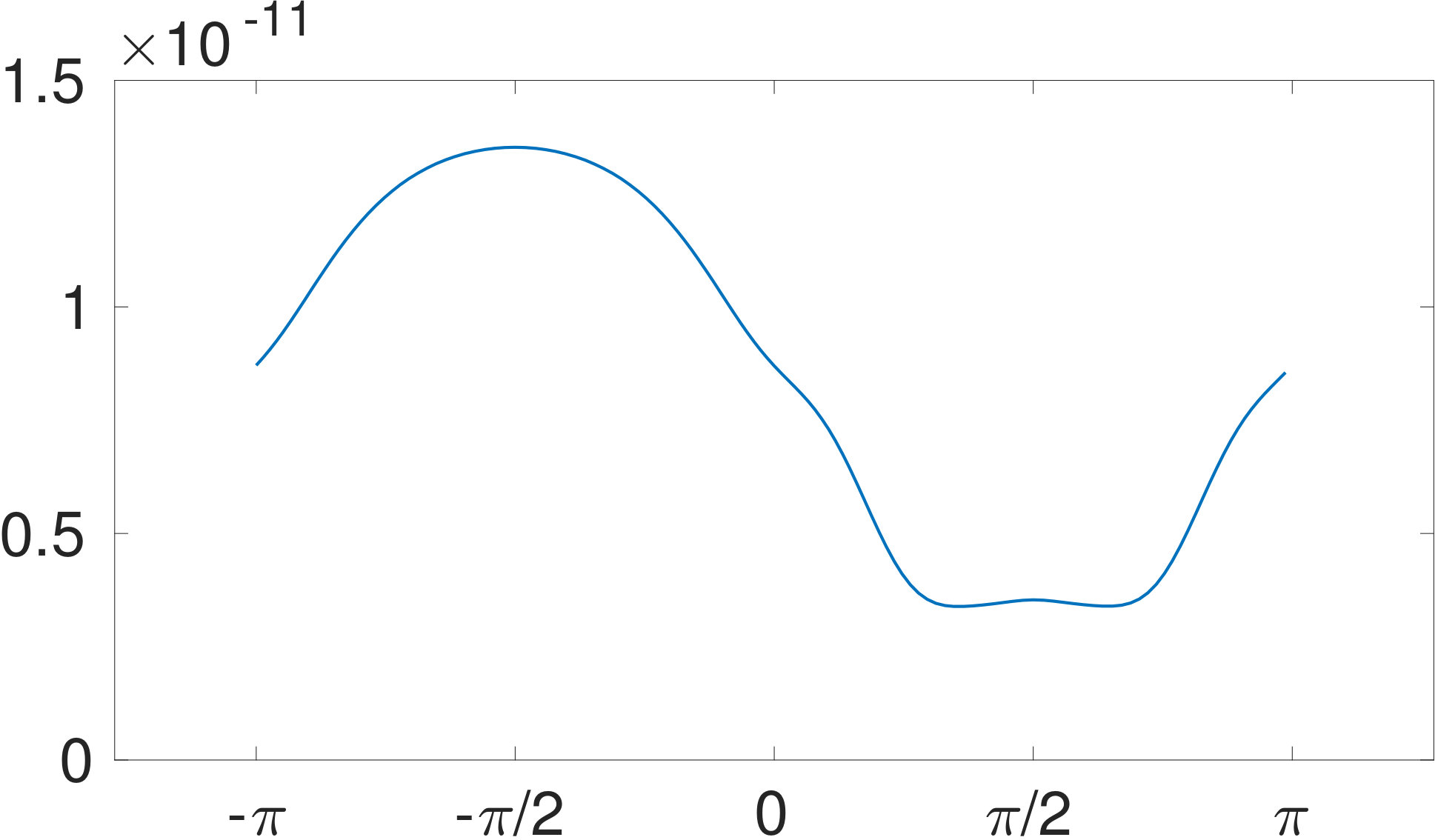 Figure 2
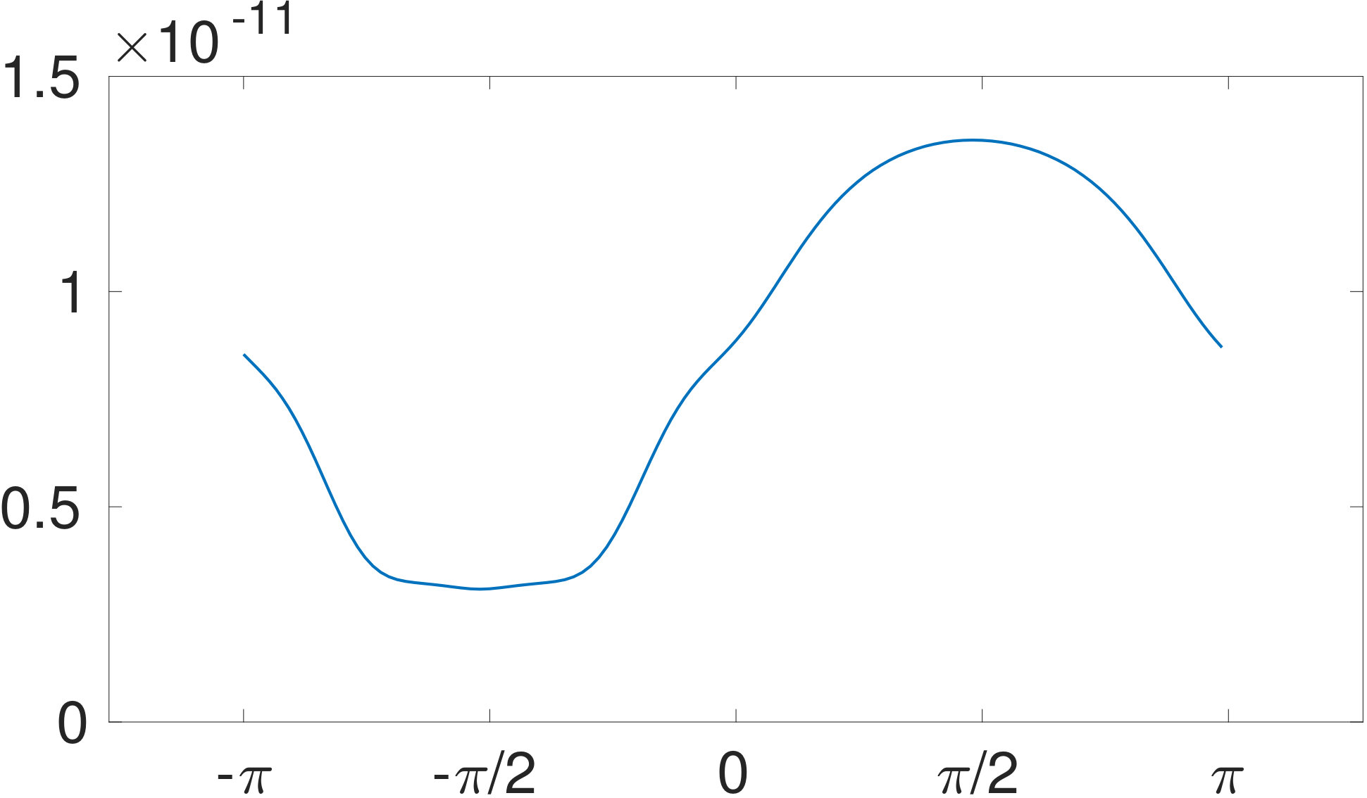 Figure 2
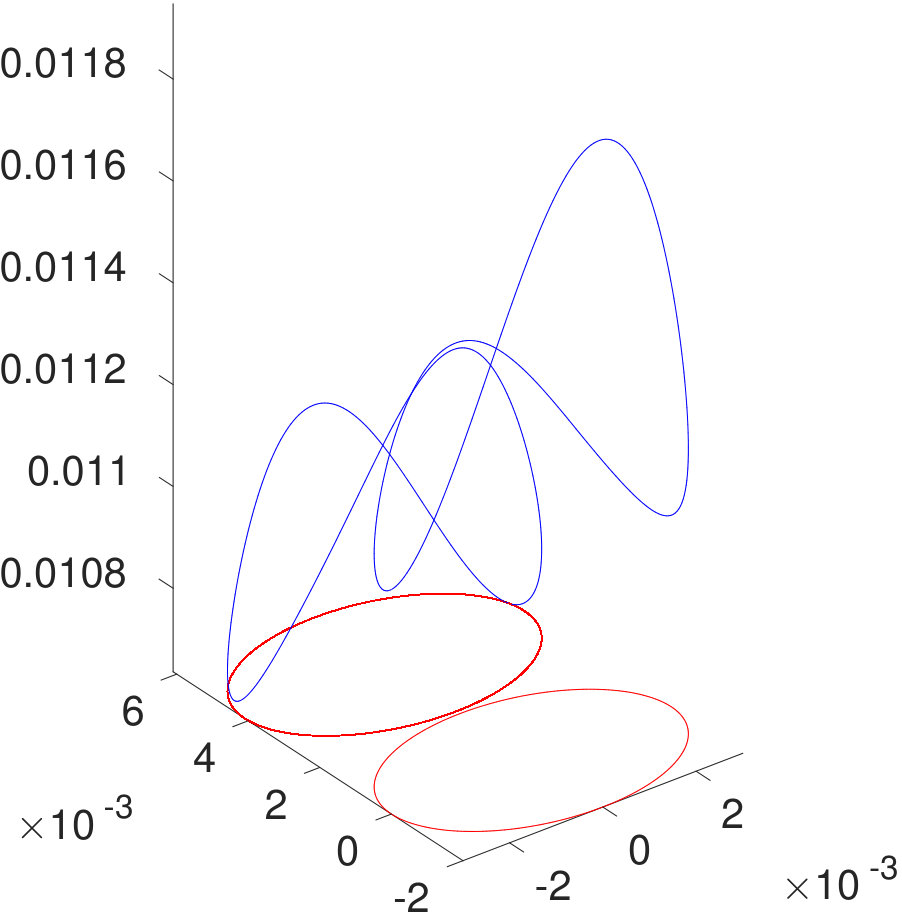 Figure 2
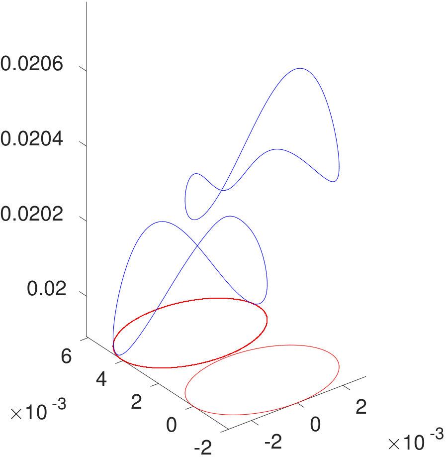 Figure 2
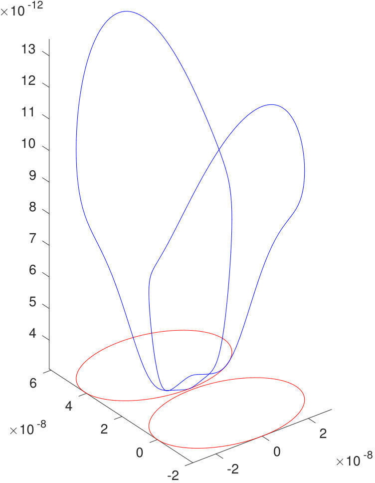 Figure 2
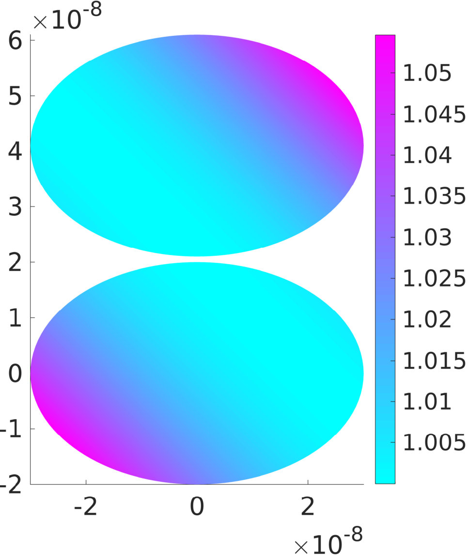 Figure 2
 Figure 2
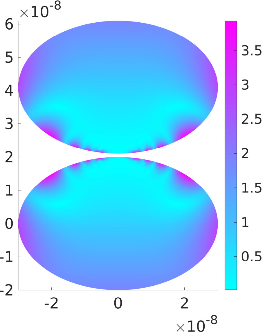 Figure 2
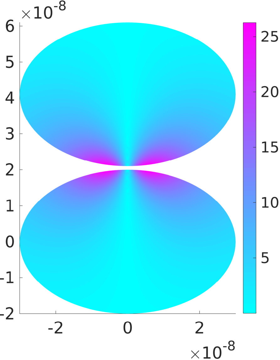 Figure 2
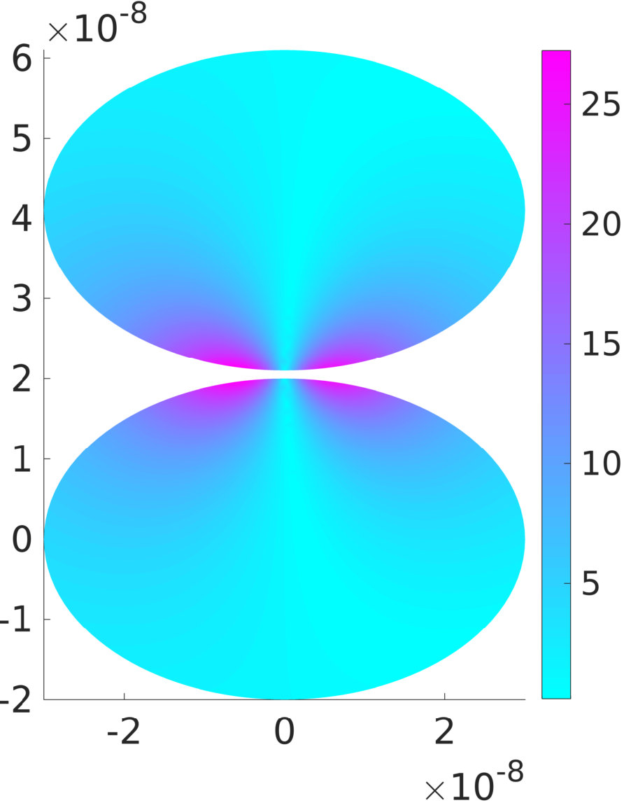 Figure 2
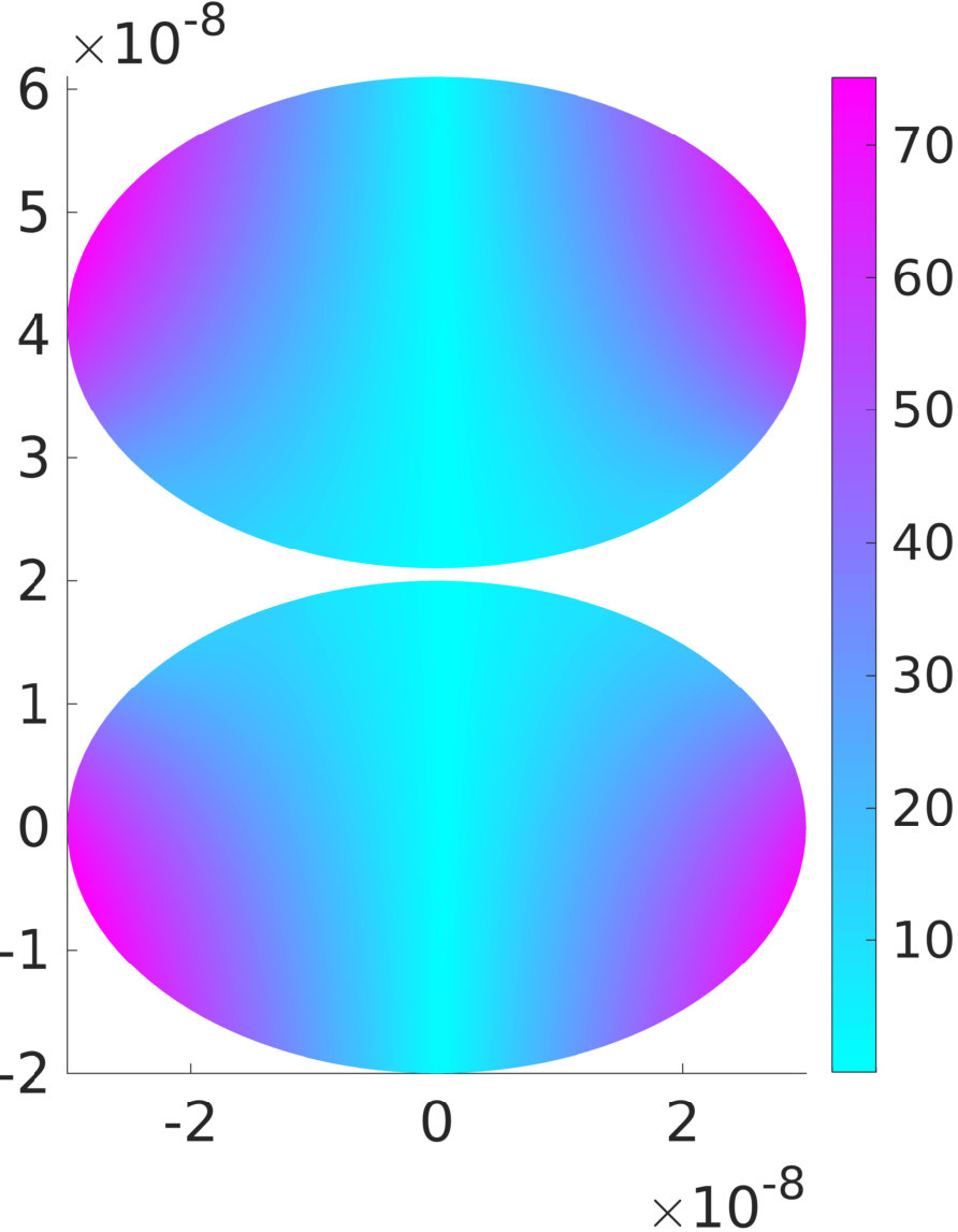 Figure 2
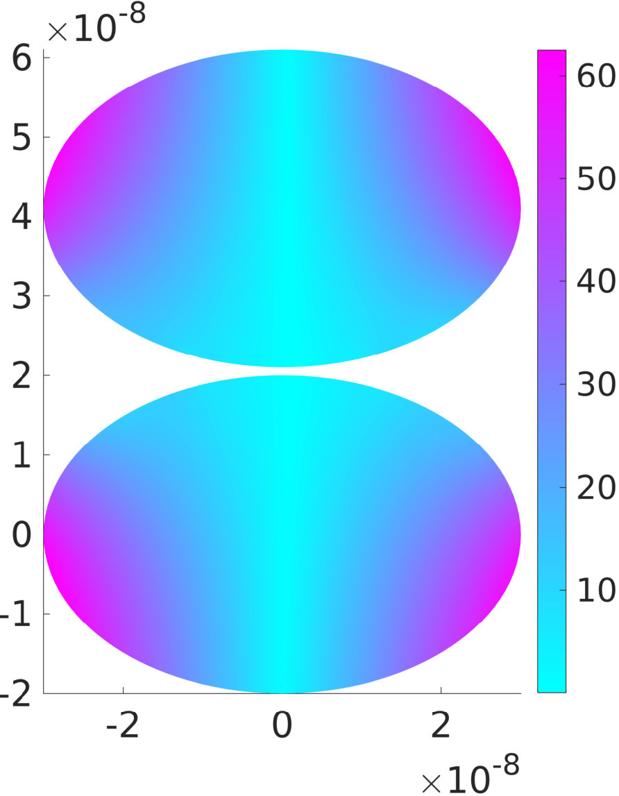 Figure 2
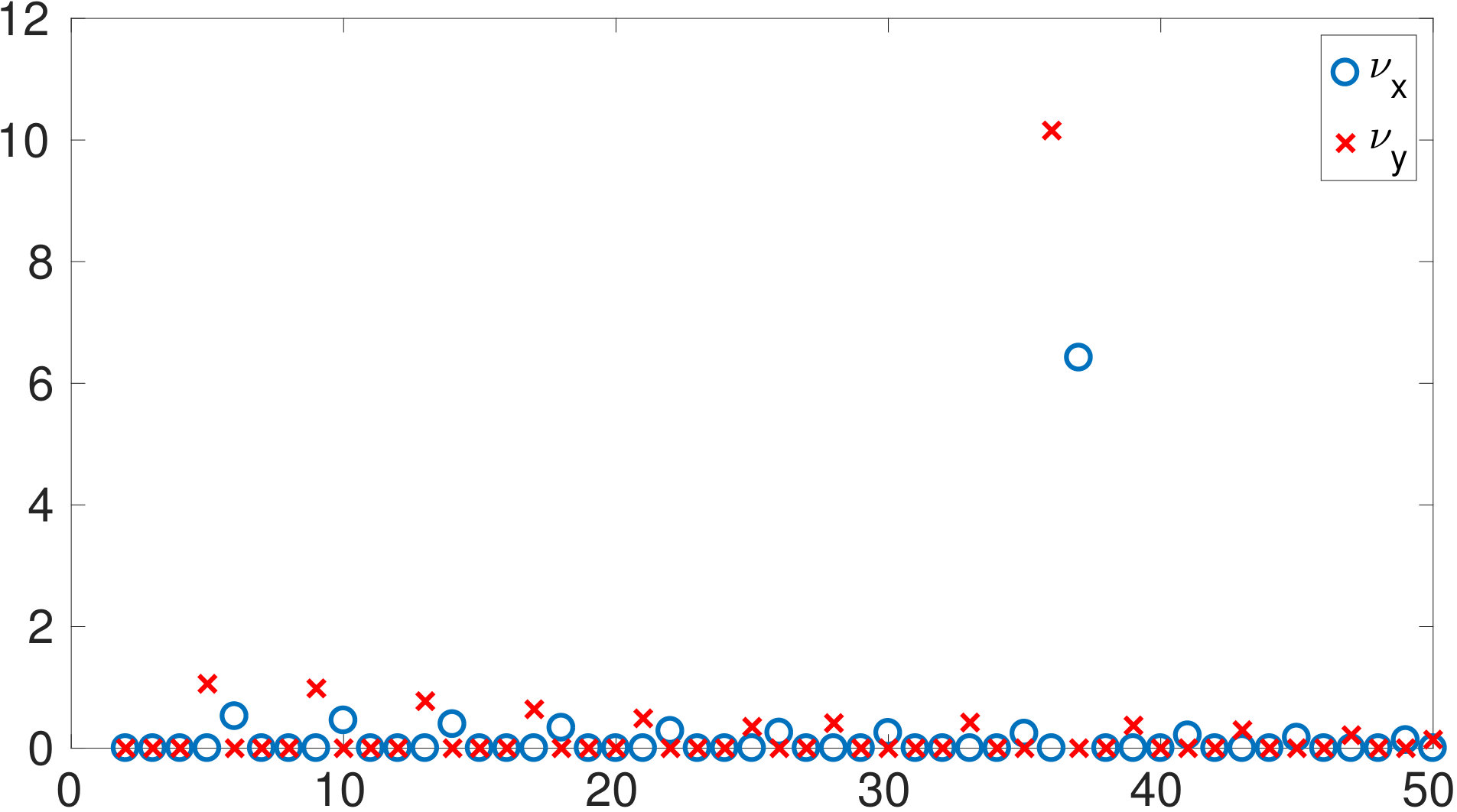 Figure 2
Peer Reviews
No public reviews on file for this paper yet. If you reviewed it on a platform where reviews are public (OpenReview, ICLR, NeurIPS, ICML), you can paste yours below so the community can read it here.
Videos
No videos yet. Explain this paper in a talk, walkthrough, or lecture? Add one.
Taxonomy
TopicsGold and Silver Nanoparticles Synthesis and Applications · Plasmonic and Surface Plasmon Research · Photoacoustic and Ultrasonic Imaging
Heat generation with plasmonic nanoparticles
Habib Ammari Department of Mathematics, ETH Zürich, Rämistrasse 101, CH-8092 Zürich, Switzerland ([email protected], [email protected]).
Francisco Romero22footnotemark: 2
Matias Ruiz Department of Mathematics and Applications, Ecole Normale Supérieure, 45 Rue d’Ulm, 75005 Paris, France ([email protected]).
Abstract
In this paper we use layer potentials and asymptotic analysis techniques to analyze the heat generation due to nanoparticles when illuminated at their plasmonic resonance. We consider arbitrary-shaped particles and both single and multiple particles. For close-to-touching nanoparticles, we show that the temperature field deviates significantly from the one generated by a single nanoparticle. The results of this paper open a door for solving the challenging problems of detecting plasmonic nanoparticles in biological media and monitoring temperature elevation in tissue generated by nanoparticle heating.
Mathematics Subject Classification (MSC2000): 35R30, 35C20.
Key words: plasmonic nanoparticle, plasmonic resonance, heat generation, Neumann-Poincaré operator.
1 Introduction
Our aim in this paper is to provide a mathematical and numerical framework for analyzing photothermal effects using plasmonic nanoparticles. A remarkable feature of plasmonic nanoparticles is that they exhibit quasi-static optical resonances, called plasmonic resonances. At or near these resonant frequencies, strong enhancement of scattering and absorption occurs [5, 7, 27]. The plasmonic resonances are related to the spectra of the non-self adjoint Neumann-Poincaré type operators associated with the particle shapes [5, 7, 8, 9, 15, 21]. Plasmonic nanoparticles efficiently generate heat in the presence of electromagnetic radiation. Their biocompatibility makes them suitable for use in nanotherapy [10].
Nanotherapy relies on a simple mechanism. First nanoparticles become attached to tumor cells using selective biomolecular linkers. Then heat generated by optically-simulated plasmonic nanoparticles destroys the tumor cells [14]. In this nanomedical application, the temperature increase is the most important parameter [23, 26]. It depends on a highly nontrivial way on the shape, the number, and organization of the nanoparticles. Moreover, it is challenging to measure it at the surface of the nanoparticles [14].
In this paper, we derive an asymptotic formula for the temperature at the surface of plasmonic nanoparticles of arbitrary shape. Our formula holds for clusters of simply connected nanoparticles. It allows to estimate the collective response of plasmonic nanoparticles.
The paper is organized as follows. In section 2 we describe the mathematical setting for the physical phenomena we are modeling. To this end, we use the Helmholtz equation to model the propagation of light which we couple to the heat equation. Later on, we present our main results in this paper which consist on original asymptotic formulas for the inner field and the temperature on the boundaries of the nanoparticles. In section 4 we prove Theorems 2.1 and 2.2. These results clarify the strong dependency of the heat generation on the geometry of the particles as it depends on the eigenvalues of the Neumann-Poincaré operator. In section 5 we present numerical examples of the temperature at the boundary of single and multiple particles. Appendix A is devoted to the asymptotic analysis of layer potentials for the Helmholtz equation in dimension two. We also include an analysis for the invertibility of the single-layer potential for the Laplacian for the case of multiple particles.
2 Setting of the problem and the main results
In this paper, we use the Helmholtz equation for modeling the propagation of light. This can be thought of as a special case of Maxwell’s equations, when the incident wave is a transverse electric or transverse magnetic (TE or TM) polarized wave. This approximation, also called paraxial approximation [19], is a good model for a laser beam which are used, in particular, in full-field optical coherence tomography. We will therefore model the propagation of a laser beam in a host domain (tissue), hosting a nanoparticle.
Let the nanoparticle occupy a bounded domain of class for some . Furthermore, let , where is centered at the origin and .
We denote by and , , the electric permittivity and magnetic permeability of the particle, respectively, both of which may depend on the frequency of the incident wave. Assume that , and that . Here and throughout, and are the permittivity and permeability of vacuum.
Similarly, we denote by and , the permittivity and permeability of the host medium, both of which do not depend on the frequency of the incident wave. Assume that and are real and strictly positive.
The index of refraction of the medium (with the nanoparticle) is given by
[TABLE]
where denotes the indicator function.
The scattering problem for a TE incident wave is modeled as follows:
[TABLE]
where denotes the outward normal derivative and is the speed of light in vacuum. We use the notation \frac{\partial}{\partial\nu}\Big{|}_{\pm} indicating
[TABLE]
with being the outward unit normal vector to .
The interaction of the electromagnetic waves with the medium produces a heat flow of energy which translates into a change of temperature governed by the heat equation [11]
[TABLE]
where is the mass density, is the thermal capacity, is the thermal conductivity, is the final time of measurements and .
We further assume that are real positive constants.
Note that in and so, outside , the heat equation is homogeneous.
The coupling of equations (2.1) and (2.2) describes the physics of our problem.
We remark that, in general, the index of refraction varies with temperature; hence, a solution to the above equations would imply a dependency on time for the electric field , which contradicts the time-harmonic assumption leading to model (2.1). Nevertheless, the time-scale on the dynamics of the index of refraction is much larger than the time-scale on the dynamics of the interaction of the electromagnetic wave with the medium. Therefore, we will not integrate a time-varying component into the index of refraction.
Let be the Green function for the Helmholtz operator satisfying the Sommerfeld radiation condition. In dimension two, is given by
[TABLE]
where is the Hankel function of first kind and order [math]. We denote .
Define the following single-layer potential and Neumann-Poincaré integral operator
[TABLE]
and
[TABLE]
Let denote the identity operator and let and respectively denote the single-layer potential and the Neumann-Poincaré operator associated to the Laplacian. Our main results in this paper are the following.
Theorem 2.1**.**
For an incident wave , the solution to (2.1), inside a plasmonic particle occupying a domain , has the following asymptotic expansion as in ,
[TABLE]
where is the outward normal to , denotes the spectrum of in and
[TABLE]
Theorem 2.2**.**
Let be the solution to (2.1). The solution to (2.2) on the boundary of a plasmonic particle occupying the domain has the following asymptotic expansion as , uniformly in ,
[TABLE]
where is the outward normal to and
[TABLE]
Remark 2.1**.**
We remark that Theorem 2.1 and Theorem 2.2 are independent. A generalization of Theorem 2.2 to is straightforward and the same type of small volume approximation can be found using the techniques presented in this paper. In fact, in , the operators involved in the first term of the temperature small volume expansion are
[TABLE]
Here is the vectorial electric field as a result of Maxwell equations. A small volume expansion for inside the nanoparticle for the plasmonic case can be found using the same techniques as those of [7].
Throughout this paper, we denote by the set of bounded linear applications from to and let and let to be the standard Sobolev space of order on .
3 Preliminaries
3.1 Layer potentials for the Helmholtz equation in two dimensions
Let us recall some properties of the single-layer potential and the Neumann-Poincaré integral operator [2]:
- (i)
is bounded; 2. (ii)
for , ; 3. (iii)
is compact; 4. (iv)
, , satisfies the Sommerfeld radiation condition at infinity; 5. (v)
\dfrac{\partial\mathcal{S}_{D}^{k}[\varphi]}{\partial\nu}\Big{|}_{\pm}=(\pm\frac{1}{2}I+(\mathcal{K}_{D}^{k})^{*})[\varphi].
We have that, for any ,
[TABLE]
with and , satisfies and satisfies the Sommerfeld radiation condition.
To satisfy the boundary transmission conditions, need to satisfy the following system of integral equations on
[TABLE]
The following result shows the existence of such a representation [4].
Theorem 3.1**.**
The operator
[TABLE]
is invertible.
4 Heat generation
In this section we consider the coupling of equations (2.1) and (2.2), that is,
[TABLE]
Under the assumption that the index of refraction does not depend on the temperature, we can solve equation (2.1) separately from equation (2.2).
Our goal is to establish a small volume expansion for the resulting temperature at the surface of the nanoparticule as a function of time. To do so, we first need to compute the electric field inside the nanoparticule as a result of a plasmonic resonance. We make use of layer potentials for the Helmholtz equation, described in subsection 3.1.
4.1 Small volume expansion of the inner field
We proceed in this section to prove Theorem 2.1.
4.1.1 Rescaling
Since we are working with nanoparticles, we want to rescale equation (3.2) to study the solution for a small volume approximation by using representation (3.1).
Recall that . For any , and for each function defined on , we introduce a corresponding function defined on as follows
[TABLE]
It follows that
[TABLE]
so system (3.2) becomes
[TABLE]
Note that the system is defined on .
For small enough is invertible (see Appendix A). Therefore,
[TABLE]
Hence, we have the following equation for :
[TABLE]
where
[TABLE]
4.1.2 Proof of Theorem 2.1
To express the solution to (2.1) in , asymptotically on the size of the nanoparticle , we make use of the representation (3.1). We derive an asymptotic expansion for on to later compute and scale back to . We divide the proof into three steps.
Step 1. We first compute an asymptotic for and .
Let be defined by (A.3) with replaced by . In , we have the following asymptotic expansion as (see Appendix A)
[TABLE]
Let be an eigenfunction of associated to the eigenvalue (see Appendix A) and let be defined by (A.6) with replaced with . Then it follows that
[TABLE]
Therefore, in ,
[TABLE]
and from the definition of we get
[TABLE]
In the same manner, in the space ,
[TABLE]
We can further develop . Indeed, for every , a Taylor expansion yields
[TABLE]
The regularity of ensures that the previous formulas hold in .
The fact that is harmonic in and Lemma A.4 imply that
[TABLE]
in .
Thus, in ,
[TABLE]
From the definition of we get
[TABLE]
Step 2. We compute .
We begin by computing an asymptotic expansion of .
The operator \mathcal{A}^{I}_{0}:=\left(\big{(}\frac{1}{2\varepsilon_{m}}+\frac{1}{2\varepsilon_{c}}\big{)}I+\big{(}\frac{1}{\varepsilon_{m}}-\frac{1}{\varepsilon_{c}}\big{)}\mathcal{K}_{B}^{*}\right) maps into . Hence, the operator defined by (which appears in the expansion of )
[TABLE]
is invertible of inverse
[TABLE]
Therefore, we can write
[TABLE]
Since is a compact self-adjoint operator in it follows that [1, 5]
[TABLE]
for a constant . Therefore, for small enough, we obtain
[TABLE]
Using the representation formula of described in Lemma A.2 we can further develop the third term in the above expression to obtain
[TABLE]
Using the same arguments as those in the proof of Lemma A.4, we have
[TABLE]
and consequently,
[TABLE]
Therefore,
[TABLE]
Step 3. Finally, we compute .
From Appendix A, the following holds when is viewed as an operator from the space to :
[TABLE]
In particular, we have
[TABLE]
It can be verified that the same expansion holds when viewed as an operator from into .
Note that the following identity holds
[TABLE]
Straightforward calculations and the fact that is harmonic in yields
[TABLE]
in . Using Lemma A.3 to scale back the estimate to leads to the desired result.
4.2 Small volume expansion of the temperature
We proceed in this section to prove Theorem 2.2. To do so, we make use of the Laplace transform method [13, 16, 22].
Consider equation (4.10) and define the Laplace transform of a function by
[TABLE]
Taking the Laplace transform of the equations on in (4.10) we formally obtain the following system:
[TABLE]
where and are the Laplace transforms of and , respectively, and .
A rigorous justification for the derivation of system (4.18) and the validity of the inverse transform of the solution can be found in [16].
Using layer potential techniques we have that, for any , defined by
[TABLE]
satisfies the differential equations in (4.18) together with the Sommerfeld radiation condition. Here , and
[TABLE]
To satisfy the boundary transmission conditions, and should satisfy the following system of integral equations on :
[TABLE]
4.2.1 Rescaling of the equations
Recall that , for any , , for each function defined on , is such that and
[TABLE]
We can also verify that
[TABLE]
Note that in the above identity, in the left-hand side we differentiate with respect to while in the right-hand side we differentiate with respect to . To simplify the notation, we will use to refer to .
We rescale system (4.20) to arrive at
[TABLE]
For small enough, is invertible (see Appendix A). Therefore, it follows that
[TABLE]
Hence, we have the following equation for :
[TABLE]
where
[TABLE]
4.2.2 Proof of Theorem 2.2
To express the solution of (2.2) on , asymptotically on the size of the nanoparticle , we make use of the representation (4.19). We will compute an asymptotic expansion for on to later compute on , scale back to and take Laplace inverse.
Using the asymptotic expansions of Appendix A the following asymptotic for holds in
[TABLE]
where
[TABLE]
In the same manner, in ,
[TABLE]
Here the remainder comes from the fact that .
Note that in and in . We can further verify that satisfies the assumption required in Lemma A.4. Thus we have
[TABLE]
where is a constant such that .
After replacing the above in the expression of we find that
[TABLE]
where
[TABLE]
Finally, in ,
[TABLE]
It can be shown, from the regularity of the remainders, that the previous identity also holds in .
Using Holder’s inequality we can prove that
[TABLE]
for some constant . Hence, we find that identity (4.25) also holds true uniformly on and , uniformly in . Scaling back to gives
[TABLE]
Before we take the inverse Laplace transform to (4.26) we note that (see [22])
[TABLE]
where and is the fundamental solution of the heat equation. In dimension two, is given by
[TABLE]
We denote . By the properties of the Laplace transform, we have
[TABLE]
We define as follows
[TABLE]
Similarly, we have that for a function
[TABLE]
We define as follows
[TABLE]
Finally, using Fubini’s theorem and taking Laplace inverse we find that
[TABLE]
uniformly in .
4.3 Temperature elevation at the plasmonic resonance
Suppose that the incident wave is , where is a unit vector. For a nanoparticle occupying a domain , the inner field solution to (2.1) is given by Theorem 2.1, which states that, in ,
[TABLE]
and hence
[TABLE]
Using Lemma A.2, we can write
[TABLE]
and therefore, for a given plasmonic frequency , we have
[TABLE]
Here is such that and the eignevalue is assumed to be simple. If this was not the case, should be replaced by the corresponding sum over an orthonormal basis of eigenfunctions for the eigenspace associated to .
Replacing in (4.29) we find
[TABLE]
Thus, at a plasmonic resonance ,
[TABLE]
Then, the temperature on the boundary of a nanoparticle at the plasmonic resonance can be estimated by plugging the above approximations of and into
[TABLE]
4.4 Temperature elevation for two close-to-touching particles
Lemma A.4 implies that
[TABLE]
Therefore, we can write the temperature on the boundary of the nanoparticle as
[TABLE]
where is the projection into : the complement in of the eigenspace associated to the eigenvalue of . This implies that, even if is close to , the quantity will remain of order , provided that the second largest eigenvalue of is not close to .
Even if this is in general the case for smooth boundaries , it turns out that for nanoparticles with two connected close-to-touching subparts with contact of order , a family of eigenvalues of in approaches as (see [12])
[TABLE]
where is the distance between connected subparts and is an increasing sequence of positive numbers.
Now, is the kind of situations encountered for metallic nanoparticles immersed in water or some biological tissue. As an example, the thermal conductivity of gold is and that of pure water is . This gives .
In view of this, the second term in (4.30) may increase considerably for some type of close-to-touching particles.
We stress, nevertheless, that this is not the general case. For a more refined analysis, asymptotics of the eigenfunctions of should be also studied.
5 Numerical results
The numerical experiments for this work can be divided into two parts. The first one is the Helmholtz equation solution approximation, which is obtained by using Theorem 2.1. The second part is the Heat equation solution computation, which is obtained using Theorem 2.2.
The major tasks surrounding the numerical implementation of these formulas are integrating against a singular kernel. The numerical computations of the operators and can be achieved by meshing the domain and integrating semi-analytically inside the triangles that are close to the singularities. We used the following formula to avoid numerical differentiation:
[TABLE]
For all the presented simulations, we considered an incident plane wave given by
[TABLE]
where is the illumination direction and is the frequency (in the red range). The considered nanoparticles are ellipses with semi-axes and , respectively.
It is worth noticing that the illumination direction is relevant solely in the asymptotic formula in Theorem 2.1. Its role is to define the coefficients of a linear combination of both components of . We will see from the numerical simulations that this is fundamental if we wish to maximize the produced electromagnetic field, and therefore the generated heat inside the nanoparticles.
With respect to the asymptotic formula established in Theorem 2.1, besides the nanoparticle’s shape , the sole parameter that is left is . For all the following simulations we will consider this as a free parameter that we will use to excite the eigenvalues of the Neumann-Poincaré operator and hence to generate resonances. The physical justification that allows us to do this is based on the Drude model [1]. Whenever we mention that we approach a particular eigenvalue of , we will adopt .
With respect to the heat equation coefficients, we use realistic values of gold for nanoparticles, and water for tissues.
5.1 Single-particle simulation
We consider one elliptical nanoparticle centered at the origin, with its semi-major axis aligned with the -axis.
5.1.1 Single-particle Helmholtz resonance
Resonance is achieved by approaching the eigenvalues of the Neumann-Poincaré operator with , and afterwards applying it to each of the components of the normal to . It turns out that for some eigenfunctions of , the normal of the shape is almost orthogonal, in , to them. Therefore, we cannot observe resonance for their associated eigenvalues; see [6]. In Figure 1 we can see values of the inner product between the eigenfunctions of and the components and of . Figure 1 suggests us which are the available resonant modes with the respective strength of each coordinate.
In Figure 2 we present the absolute value of the inner field for the first three resonant modes, corresponding to the second, third and sixth eigenvalue of , respectively. In Figure 3 we decompose the inner field into the zeroth-order and the first-order terms respectively given by and \mathcal{S}_{D}\big{(}\lambda_{\varepsilon}I-\mathcal{K}_{D}^{*}\big{)}^{-1}[\nu]\cdot\nabla u^{i}(z). Figure 4 shows the components of the vector .
From Figure 3, we can see that when we excite the nanoparticle at its resonant mode, the largest contribution to the electromagnetic field comes from the first-order term of the small volume expansion formula established in Theorem 2.1.
Observing the vectorial components of the first-order term in Figure 4 tells us how important is the illumination direction as the -component is significantly stronger than the -component. If we wish to maximize the electromagnetic field and therefore the generated heat, the recommended illumination direction would be around (with being the transpose), as it was initially suggested by Figure 1.
5.1.2 Single-particle surface heat generation
Considering the electromagnetic field inside the nanoparticle given by the first resonant mode presented in Figure 2, following the formula given by Theorem 2.2, we compute the generated heat on the surface of the nanoparticle. In Figure 5 we plot the generated heat in three dimensions and present a two dimensional plot obtained by parameterizing the boundary. In Figure 6 we decompose the heat in its first- and second-order terms given by formula 2.2, being and respectively. In Figure 7, we integrate the total heat on the boundary and plot it as a function of time, for each component.
We can observe that the heat is not symmetric, this can be noticed from the total inner field for the first resonance mode in Figure 2. The reason behind this non symmetry is because we are illuminating with direction over an ellipse. From Figure 7 we can notice that the first-order term converges, while the zeroth-order term increases logarithmically, as it is expected from the known solution of the heat equation for constant source in two dimensions that the heat increases logarithmically.
5.2 Two particles simulation
We consider two elliptical nanoparticles , , , with the same shape and orientation as the nanoparticle considered in the above example. The particle is centered at the origin and is centered at , resulting in a separation distance of between the two particles.
5.2.1 Two particles Helmholtz resonance
Following the same analysis as the one for one particle, in Figure 8 we present the inner product between the eigenvectors of with each component of the normal of . We can observe that there are more available resonant modes. In particular we can see that when approaches the 36th or 37th eigenvalues, we achieve strong resonant modes.
In Figure 2 we present the absolute value of the inner field for the resonant modes corresponding to the 6th, 37th and 38th eigenvalues of . Similarly to the case with one particle, the dominant term in the electromagnetic field for each case is the first-order term. In Figure 10 we decompose the first-order term in its -component and -component.
As suggested by Figure 8, for the resonant mode associated to the 38th eigenvector of , the stronger component is the one on the y direction, meaning that if we wish to maximize the electromagnetic field, and therefore the generated heat, it is suggested to consider the illumination vector .
5.2.2 Two particles surface heat generation
Similarly to the analysis carried out for one particle, we now compute the generated heat for these two particles while undergoing resonance for the resonant mode associated to the 38th eigenvalue of . In Figure 11 we plot generated heat in the boundary of the two nanoparticles. In Figure 12 we decompose the generated heat in its zeroth and first-order component, explicited for each of the two nanoparticles.
Similarly to the single nanoparticle case, there is no symmetry on the heat values on the boundary, which is due to the illumination. We have not provided the plots of the heat integrated along the boundary, as the conclusions are the same as the ones in the single nanoparticle case: The total heat on the boundary increases logarithmically, initially on time the dominant term is the fist-order one, but as time increases the zeroth-order term becomes the predominant one.
6 Concluding remarks
In this paper we have derived asymptotic formula for the temperature elevation due to plasmonic nanoparticles. We have considered thermal coupling within close-to-touching nanoparticles, where the temperature field deviates significantly from the one generated by a single nanoparticle. Our results can be used for the thermal detection and localization of the nanoparticles [24]. They can also be used for monitoring temperature elevation due to plasmonic nanoparticles based on the photoacoustic signal recently analyzed in [28]. Thermoacoustic signals generated by nanoparticle heating can be computed numerically based on the successive resolution of the thermal diffusion problem considered in this paper and a thermoelastic problem, taking into account the size and shape of the nanoparticle, thermoelastic and elastic properties of both the particle and its environment, and the temperature-dependence of the thermal expansion coefficient of the environment. For sufficiently high illumination fluences, this temperature dependence yields a nonlinear relationship between the photoacoustic amplitude and the fluence [25]. The investigation of this nonlinear model will be the subject of a forthcoming publication.
Appendix A Asymptotic analysis of the single-layer potential in two dimensions
In this section we make an analysis of the single-layer potential for small values of , i.e . We use this, in section 4.1 , to make and expansion on of the operator and its inverse.
The results in this section were first established in [8] for a connected domain . Here we generalize them to non connected domains.
A.1 Layer potentials for the Laplacian in two dimensions
Recall the definition of the single-layer potential and Neumann-Poincaré operators for the Laplacian:
[TABLE]
In the single-layer potential is not, in general, invertible. Hence, does not define an inner product and the symmetrization technique described in [2, subsection 2.1.4] is no longer valid.
Here and throughout, denotes the duality pairing between and .
To overcome this difficulty, we will introduce a substitute of , in the same way as in [8].
We first need the following lemma.
Lemma A.1**.**
Let . We have .
Proof.
It is known that
[TABLE]
is invertible [3, Theorem 2.26].
We can see that , where . The invertibility of implies that . Thus, by the range theorem we have
[TABLE]
∎
Definition A.1**.**
We call the unique element of such that .
Note that for every we have the decomposition
[TABLE]
where we can see that . This kind of decomposition, , with is unique.
Note that we can decompose as a direct sum of elements with zero-mean and multiples of , . This allows us to define the following operator.
Definition A.2**.**
Let be the linear operator that satisfies
[TABLE]
Remark A.1**.**
When is invertible, is similar enough to keep the invertibility. When is not invertible, then and the operator becomes an invertible alternative to that images the kernel to the space .
Remark A.2**.**
* follows the same definition.*
Theorem A.1**.**
* is invertible, self-adjoint and negative for and satisfies the following Calderón identity: .*
Proof.
The invertibility is a direct consequence of Lemma A.1.
Indeed, since is Fredholm of zero index, so is . Therefore, we only need the injectivity. Suppose that, such that . This mean that, such that . Therefore, , which is a contradiction. Hence .
The self-adjointness comes directly form that of . Noticing that is an eigenfunction of eigenvalue of we get the Calderón identity from a similar one satisfied by : ; see [2, Lemma 2.12].
It is known that if and , see [2, Lemma 2.10]. Therefore, writing \varphi=\psi+\Big{(}\int_{\partial D}\varphi d\sigma\Big{)}\varphi_{0}, with \psi=\varphi-\Big{(}\int_{\partial D}\varphi d\sigma\Big{)}\varphi_{0}, and noticing that , we have
[TABLE]
if .
∎
Definition A.3**.**
We define the space as the Hilbert space resulting from endowing with the inner product
[TABLE]
Similarly, we let to be the Hilbert space resulting from endowing with the inner product
[TABLE]
If is , we have the following result.
Lemma A.2**.**
Let be a bounded domain of and let be the operator introduced in Definition A.2. Then
- (i)
The operator is compact self-adjoint in the Hilbert space and is equivalent to ; Similarly, the Hilbert space is equivalent to . 2. (ii)
*Let , be the eigenvalue and normalized eigenfunction pair of with . Then, and as ; * 3. (iii)
The following representation formula holds: for any ,
[TABLE]
The following lemmas are needed in the proof of Theorem 2.1 and Theorem 2.2.
Lemma A.3**.**
Let and be the function such that, for every , , for almost all . Then
[TABLE]
Similarly, if for every , , for almost all , then
[TABLE]
Proof.
We only prove the scaling in . From the proof of Theorem A.1, we have
[TABLE]
where \psi=\varphi-\Big{(}\int_{\partial D}\varphi d\sigma\Big{)}\varphi_{0}. Note that and so, as well.
By a rescaling argument we find that
[TABLE]
∎
Lemma A.4**.**
Let be such that with . Then, in ,
[TABLE]
For some and for a constant .
Moreover, if , in , , then
[TABLE]
with
[TABLE]
where is given in Definition A.1. Here, by an abuse of notation, we still denote by the trace of on .
Proof.
Let . Then
[TABLE]
We have used the fact that is harmonic in .
Consider the linear application . We have
[TABLE]
Here we have used Holder’s inequality, a standard Sobolev embedding, the trace theorem and the fact that is continuous. By the Riez representation theorem, there exists such that .
By abuse of notation we still denote to make explicit the dependency on . It follows that
[TABLE]
We now show that in , .
Indeed, let , then
[TABLE]
Here we have used the assumption on , the fact that is harmonic in and and that for we have and for .
Therefore,
[TABLE]
Finally, recaling the definition of given in Definition A.1 we obtain that
[TABLE]
∎
A.2 Asymptotic expansions
Let us now consider the single-layer potential for the Helmholtz equation in given by
[TABLE]
where and is the Hankel function of first kind and order [math]. We have, for ,
[TABLE]
where
[TABLE]
and is the Euler constant. Thus, we get
[TABLE]
where
[TABLE]
Lemma A.5**.**
The norms and are uniformly bounded with respect to . Moreover, the series in (A.4) is convergent in for .
Observe that
[TABLE]
Then it follows that
[TABLE]
where
[TABLE]
Therefore, we arrive at the following result.
Lemma A.6**.**
For small enough, is invertible.
Proof.
is clearly a compact operator. Since is invertible, the invertibility of is equivalent to that of . By the Fredholm alternative, we only need to prove the injectivity of .
Since , for , we need to show that .
We have
[TABLE]
Since we can always find a small enough such that , we need . This yields the stated result. ∎
Lemma A.7**.**
For small enough, the operator is invertible.
Proof.
The operator is a compact operator. Because is invertible for small enough, by the Fredholm alternative only the injectivity of is necessary. From the uniqueness of a solution to the Helmholtz equation we get the result. ∎
Lemma A.8**.**
The following asymptotic expansion holds for small enough:
[TABLE]
with
[TABLE]
Note that .
Proof.
We can write (A.4) as
[TABLE]
where . From Lemma A.6 and Lemma A.7 we get the identity
[TABLE]
Hence, we have
[TABLE]
Here,
[TABLE]
Then,
[TABLE]
and therefore,
[TABLE]
It is clear that is bounded for small. Since goes to zero as goes to zero, for small enough, we can write
[TABLE]
which yields the desired result. ∎
We now consider the expansion for the boundary integral operator . We have
[TABLE]
where
[TABLE]
Lemma A.9**.**
The norms and are uniformly bounded for . Moreover, the series in (A.7) is convergent in .
The reference list from the paper itself. Each links out to its DOI / PubMed record.
- 1[1] H. Ammari, Y. Deng, and P. Millien, Surface plasmon resonance of nanoparticles and applications in imaging, Arch. Ration. Mech. Anal., 220 (2016), 109–153.
- 2[2] H. Ammari, J. Garnier, W. Jing, H. Kang, M. Lim, K. Sølna, and H. Wang, Mathematical and Statistical Methods for Multistatic Imaging , Lecture Notes in Mathematics, Volume 2098, Springer, Cham, 2013.
- 3[3] H. Ammari and H. Kang, Polarization and Moment Tensors with Applications to Inverse Problems and Effective Medium Theory , Applied Mathematical Sciences, Vol. 162, Springer-Verlag, New York, 2007.
- 4[4] H. Ammari, H. Kang, Boundary Layer Techniques for Solving the Helmholtz Equation in the Presence of Small Inhomogeneities. Journal of Mathematical Analysis and Applications 296 (2004), no. 1, 190-208.
- 5[5] H. Ammari, P. Millien, M. Ruiz, and H. Zhang, Mathematical analysis of plasmonic nanoparticles: the scalar case, Arch. Rational Mech. Anal., DOI: 10.1007/s 00205-017-1084-5.
- 6[6] H. Ammari, M. Putinar, M. Ruiz, S. Yu, and H. Zhang, Shape reconstruction of nanoparticles from their associated plasmonic resonances, ar Xiv: 1602.05268.
- 7[7] H. Ammari, M. Ruiz, S. Yu, and H. Zhang, Mathematical analysis of plasmonic resonances for nanoparticles: the full Maxwell equations, J. Differential Equations, 261 (2016), 3615–3669.
- 8[8] K. Ando and H. Kang, Analysis of plasmon resonance on smooth domains using spectral properties of the Neumann-Poincaré operator, J. Math. Anal. Appl., 435 (2016), 162–178.