The Long-Moody construction and polynomial functors
Arthur Soulié
Abstract
In 1994, Long and Moody gave a construction on representations of
braid groups which associates a representation of Bn
with a representation of Bn+1. In this paper, we prove
that this construction is functorial and can be extended: it inspires
endofunctors, called Long-Moody functors, between the category of
functors from Quillen’s bracket construction associated with the braid
groupoid to a module category. Then we study the effect of Long-Moody
functors on strong polynomial functors: we prove that they increase
by one the degree of very strong polynomiality.
††footnotetext: Published in Annales de l’Institut Fourier, Volume 69 (2019) no. 4 p. 1799-1856.
This work was partially supported by the ANR Project ChroK, ANR-16-CE40-0003.
2010 Mathematics Subject Classification:
18D10, 18A25, 20C07, 20C99, 20J99, 20F36, 20F38, 57M07, 57N05.
Keywords: braid groups, functor categories, Long-Moody construction, polynomial functors.
Introduction
Linear representations of the Artin braid group on n strands Bn
is a rich subject which appears in diverse contexts in mathematics
(see for example [5] or [19] for
an overview). Even if braid groups are of wild representation type,
any new result which allows us to gain a better understanding of them
is a useful contribution.
In 1994, as a result of a collaboration with Moody in [17],
Long gave a method to construct from a linear representation ρ:Bn+1→GL(V)
a new linear representation LM(ρ):Bn→GL(V⊕n)
of Bn (see [17, Theorem 2.1]). Moreover, the
construction complicates in a sense the initial representation. For
example, applying it to a one dimensional representation of Bn+1,
the construction gives a mild variant of the unreduced Burau representation
of Bn. This method was in fact already implicitly present
in two previous articles of Long dated 1989 (see [15, 16]).
In the article [3] dating from 2008, Bigelow and
Tian consider the Long-Moody construction from a matricial point of
view. They give alternative and purely algebraic proofs of some results
of [17], and they slightly extend some of them. In a survey
on braid groups (see the Open Problem 7 in [5]),
Birman and Brendle underline the fact that the Long-Moody construction
should be studied in greater detail.
Our work focuses on the study of the Long-Moody construction LM
from a functorial point of view. More precisely, we consider the category
Uβ associated with braid groups.
This category is an example of a general construction due to Quillen
(see [9]) on the braid groupoid β.
In particular, the category Uβ
has natural numbers N as objects. For each natural number
n, the automorphism group AutUβ(n)
is the braid group Bn. Let K-Mod
be the category of K-modules, with K a commutative
ring, and Fct(Uβ,K-Mod)
be the category of the functors from Uβ
to K-Mod. An object M of Fct(Uβ,K-Mod)
gives by evaluation a family of representations of braid groups {Mn:Bn→GL(M(n))}n∈N,
which satisfies some compatibility properties (see Section 1.1).
Randal-Williams and Wahl use the category Uβ
in [20] to construct a general framework to
prove homological stability for braid groups with twisted coefficients.
Namely, they obtain the stability for twisted coefficients given by
objects of Fct(Uβ,K-Mod).
In Proposition 2.21, we prove that a version of the
Long-Moody construction is functorial. We fix two families of morphisms
{an:Bn→Aut(Fn)}n∈N
and {ςn:Fn→Bn+1}n∈N,
satisfying some coherence properties (see Section 2.1).
Once this framework set, we show:
**Theorem A ****(Proposition 2.21) **.
There is a functor LMa,ς:Fct(Uβ,K-Mod)→Fct(Uβ,K-Mod),
called the Long-Moody functor with respect to coherent families of
morphisms {an}n∈N and {ςn}n∈N,
which satisfies for σ∈Bn and M∈Obj(Fct(Uβ,K-Mod))
[TABLE]
Among the objects in the category Fct(Uβ,K-Mod)
the strong polynomial functors play a key role. This notion extends
the classical one of polynomial functors, which were first defined
by Eilenberg and Mac Lane in [8] for functors
on module categories, using cross effects. This definition can also
be applied to monoidal categories where the monoidal unit is a null
object. Djament and Vespa introduce in [7] the definition
of strong polynomial functors for symmetric monoidal categories with
the monoidal unit being an initial object. Here, the category Uβ
is neither symmetric, nor braided, but pre-braided in the sense of
[20]. However, we show that the notion of strong
polynomial functor extends to the wider context of pre-braided monoidal
categories (see Definition 3.4). We also introduce the
notion of very strong polynomial functor (see Definition 3.16).
Strong polynomial functors turn out inter alia to be very useful for
homological stability problems. For example, in [20],
Randal-Williams and Wahl prove their homological stability results
for twisted coefficients given by a specific kind of strong polynomial
functors, namely coefficient systems of finite degree (see [20, Section 4.4]).
We investigate the effects of Long-Moody functors on very strong polynomial
functors. We establish the following theorem, under some mild additional
conditions (introduced in Section 4.1.1)
on the families of morphisms {an}n∈N*
*and {ςn}n∈N,
which are then said to be reliable.
Theorem B** (Corollary 4.27) **.
Let M be a very strong polynomial functor of Fct(Uβ,K-Mod)
of degree n and let {an}n∈N
and {ςn}n∈N be coherent
reliable families of morphisms. Then, considering the Long-Moody functor
LMa,ς with respect to the morphisms {an}n∈N
and {ςn}n∈N, LMa,ς(M)
is a very strong polynomial functor of degree n+1.
Thus, iterating the Long-Moody functor on a very strong polynomial
functor of Fct(Uβ,K-Mod)
of degree d, we generate polynomial functors of Fct(Uβ,K-Mod),
of any degree bigger than d. For instance, Randal-Williams and
Wahl define in [20, Example 4.3] a functor
Burt:Uβ→C[t±1]-Mod
encoding the unreduced Burau representations. Similarly, we introduce
a functor TYMt:Uβ→C[t±1]-Mod
corresponding to the representations considered by Tong, Yang and
Ma in [22]. These functors Burt and TYMt
are very strong polynomial of degree one (see Proposition 3.25),
and moreover, we prove that the functor Burt is equivalent
to a functor obtained by applying the Long-Moody construction. Thus,
the Long-Moody functors will provide new examples of twisted coefficients
corresponding to the framework of [20].
This construction is extended in the forthcoming work [21]
for other families of groups, such as automorphism groups of free
groups, braid groups of surfaces, mapping class groups of orientable
and non-orientable surfaces or mapping class groups of 3-manifolds.
The results proved here for (very) strong polynomial functors will
also hold in the adapted categorical framework for these different
families of groups.
The paper is organized as follows. Following [20],
Section 1 introduces the category Uβ
and gives first examples of objects of Fct(Uβ,K-Mod).
Then, in Section 2, we introduce the
Long-Moody functors, prove Theorem A and give some of their properties.
In Section 3, we review the notion
of strong polynomial functors and extend the framework of [7]
to pre-braided monoidal categories. Finally, Section 4
is devoted to the proof of Theorem B and to some other properties
of these functors. In particular, we tackle the Open Problem 7
of [5].
Notation 0.1*.*
We will consider a commutative ring
K throughout this work. We denote by K-Mod
the category of K-modules. We denote by Gr
the category of groups. We take the convention that the set of natural
numbers N is the set of nonnegative integers {0,1,2,…}.
Let Cat denote the category of small categories. Let
C be an object of Cat. We use the abbreviation
Obj(C) to denote the objects of C.
For D a category, we denote by Fct(C,D)
the category of functors from C to D.
If [math] is initial object in the category C, then we
denote by ιA:0→A the unique morphism from [math]
to A. The maximal subgroupoid Gr(C)
is the subcategory of C which has the same objects as
C and of which the morphisms are the isomorphisms of
C. We denote by Gr:Cat→Cat
the functor which associates to a category its maximal subgroupoid.
Acknowledgement*.*
The author wishes to thank most sincerely his PhD advisor Christine
Vespa, and Geoffrey Powell, for their careful reading, corrections,
valuable help and expert advice. He would also especially like to
thank Aurélien Djament, Nariya Kawazumi, Martin Palmer, Vladimir Verchinine
and Nathalie Wahl for the attention they have paid to his work, their
comments, suggestions and helpful discussions. Additionally, he would
like to thank the anonymous referee for his reading of this paper.
Contents
-
1 The category Uβ
-
1.1 Quillen’s bracket construction associated with the groupoid β
-
1.1.1 Generalities
-
1.1.2 Pre-braided monoidal category
-
1.2 Examples of functors associated with braid representations
-
2 Functoriality of the Long-Moody construction
-
2.1 Braid groups and free groups
-
2.2 The Long-Moody functors
-
2.3 Evaluation of the Long-Moody functor
-
2.3.1 Computations for LM1
-
2.3.2 Computations for other cases
-
3 Strong polynomial functors
-
3.1 Strong polynomiality
-
3.2 Very strong polynomial functors
-
3.3 Examples of polynomial functors over Uβ
-
4 The Long-Moody functor applied to polynomial functors
-
4.1 Decomposition of the translation functor
-
4.1.1 Additional conditions
-
4.1.2 The intermediary functors
-
4.1.3 Splitting of the translation functor
-
4.2 Splitting of the difference functor
-
4.3 Increase of the polynomial degree
-
4.4 Other properties of the Long-Moody functors
1 The category Uβ
The aim of this section is to describe the category Uβ
associated with braid groups that is central to this paper. On the
one hand, we recall some notions and properties about Quillen’s construction
from a monoidal groupoid and pre-braided monoidal categories introduced
by Randal-Williams and Wahl in [20]. On the
other hand, we introduce examples of functors over the category Uβ.
We recall that the braid group on n≥2 strands denoted by Bn
is the group generated by σ1, …, σn−1 satisfying
the relations:
∀i∈{1,…,n−2}, σiσi+1σi=σi+1σiσi+1;
∀i,j∈{1,…,n−1} such that ∣i−j∣≥2,
σiσj=σjσi.
B0 and B1 both are the trivial group.
The family of braid groups is associated with the following groupoid.
Definition 1.1**.**
The braid groupoid β
is the groupoid with objects the natural numbers n∈N
and morphisms (for n,m∈N):
[TABLE]
Remark 1.2*.*
The composition of morphisms ∘ in the groupoid β
corresponds to the group operation of the braid groups. So we will
abuse the notation throughout this work, identifying σ∘σ′=σσ′
for all elements σ and σ′ of Bn with
n∈N (with the convention that we read from the right
to the left for the group operation).
1.1 Quillen’s bracket construction associated with the groupoid β
This section focuses on the presentation and the study of Quillen’s
bracket construction Uβ (see [9, p.219])
on the braid groupoid β. It associates to β
a monoidal category whose unit is initial. The category Uβ
has further properties: Quillen’s bracket construction on β
is a pre-braided monoidal category (see Section 1.1.2)
and β is its maximal subgroupoid. For an introduction
to (braided) strict monoidal categories, we refer to [18, Chapter XI].
Notation 1.3*.*
A strict monoidal category will be denoted by (C,♮,0),
where C is the category, ♮ is the monoidal
product and [math] is the monoidal unit.
1.1.1 Generalities
In [20], Randal-Williams and Wahl study a construction
due to Quillen in [9, p.219], for a monoidal category
S acting on a category X in the case S=X=G where
G is a groupoid. It is called Quillen’s bracket construction.
Our study here is based on [20, Section 1]
taking G=β.
Definition 1.4**.**
[18, Chapter XI, Section 4] A
monoidal product ♮:β×β⟶β
is defined by the usual addition for the objects and laying two braids
side by side for the morphisms. The object [math] is the unit of this
monoidal product. The strict monoidal groupoid (β,♮,0)
is braided, its braiding is denoted by b−,−β.
Namely, the braiding is defined for all natural numbers n and m
such that n+m≥2 by:
[TABLE]
where {σi}i∈{1,…,n+m−1}
denote the Artin generators of the braid group Bn+m.
We consider the strict monoidal groupoid (β,♮,0)
throughout this section.
Definition 1.5**.**
[20, Section 1.1] Quillen’s
bracket construction on the groupoid β, denoted
by Uβ, is the category defined by:
Objects: Obj(Uβ)=Obj(β)=N;
Morphisms: for n and n′ two objects of β,
the morphisms from n to n′ in the category Uβ
are given by:
[TABLE]
In other words, a morphism from n to n′ in the category Uβ,
denoted by [n′−n,f]:n→n′, is an equivalence
class of pairs (n′−n,f) where n′−n is an object of
β, f:(n′−n)♮n→n′
is a morphism of β, in other words an element
of Bn′. The equivalence relation ∼ is defined
by (n′−n,f)∼(n′−n,f′) if and only if there
exists an automorphism g∈Autβ(n′−n)
such that the following diagram commutes.
[TABLE]
For all objects n of Uβ, the identity
morphism in the category Uβ is given
by [0,idn]:n→n.
Let [n′−n,f]:n→n′ and [n′′−n′,g]:n′→n′′
be two morphisms in the category Uβ.
Then, the composition in the category Uβ
is defined by:
[TABLE]
The relationship between the automorphisms of the groupoid β
and those of its associated Quillen’s construction Uβ
is actually clear. First, let us recall the following notion.
Definition 1.6**.**
Let (G,♮,0)
be a strict monoidal category. It has no zero divisors if for all
objects A and B of G, A♮B≅0 if
and only if A≅B≅0.
The braid groupoid (β,♮,0) has
no zero divisors. Moreover, by Definition 1.1,
Autβ(0)={id0}. Hence, we
deduce the following property from [20, Proposition 1.7].
Proposition 1.7**.**
The groupoid β is the maximal subgroupoid of Uβ.
In addition, Uβ has the additional
useful property.
Proposition 1.8**.**
[20, Proposition 1.8 (i)]** The unit [math] of
the monoidal structure of the groupoid (β,♮,0)
is an initial object in the category Uβ.
Remark 1.9*.*
Let n be a natural number and ϕ∈Autβ(n).
Then, as an element of HomUβ(n,n),
we will abuse the notation ϕ=[0,ϕ]. This comes
from the canonical functor:
[TABLE]
Finally, we are interested in a way to extend an object of Fct(β,K-Mod)
to an object of Fct(Uβ,K-Mod).
This amounts to studying the image of the restriction Fct(Uβ,K-Mod)→Fct(β,K-Mod).
Proposition 1.10**.**
Let M be an object
of Fct(β,K-Mod).
Assume that for all n,n′,n′′∈N such that n′′≥n′≥n,
there exists an assignment M([n′−n,idn′]):M(n)→M(n′)
such that:
[TABLE]
Then, we define a functor M:Uβ→K-Mod
(assigning M([n′−n,σ])=M(σ)∘M([n′−n,idn′])
for all [n′−n,σ]∈HomUβ(n,n′))
if and only if for all n,n′∈N such that n′≥n:
[TABLE]
for all σ∈Bn and all ψ∈Bn′−n.
Remark 1.11*.*
Note that for n′=n, M([n′−n,idn′])=IdM(n).
Proof of Proposition 1.10.
Let us assume that relation (2)
is satisfied. We have to show that the assignment on morphisms is
well-defined with respect to Uβ. First,
let us prove that our assignment conforms with the defining equivalence
relation of Uβ (see Definition 1.5).
For n and n′ natural numbers such that n′≥n, let us consider
[n′−n,σ] and [n′−n,σ′] in HomUβ(n,n′)
such that there exists ψ∈Bn′−n so that σ′∘(ψ♮idn)=σ.
Since M is a functor over β, M([n′−n,σ])=M(σ′)∘(M(ψ♮idn)∘M([n′−n,idn′])).
According to the relation (2) and since M satisfies
the identity axiom, we deduce that M([n′−n,σ])=M(σ′)∘M(ψ♮idn)∘M([n′−n,idn′])=M([n′−n,σ′]).
Now, we have to check the composition axiom. Let n, n′ and n′′
be natural numbers such that n′′≥n′≥n, let ([n′−n,σ])
and ([n′′−n′,σ′]) be morphisms respectively
in HomUβ(n,n′) and in
HomUβ(n′,n′′). By our
assignment and composition in Uβ (see
Definition 1.5) we have that:
[TABLE]
According to the relation (2), we deduce that:
[TABLE]
Hence, it follows from relation (1) that:
[TABLE]
Conversely, assume that the functor M:Uβ→K-Mod
is well-defined. In particular, composition axiom in Uβ
is satisfied and implies that for all n,n′∈N such that
n′≥n, for all σ∈Bn:
[TABLE]
It follows from the defining equivalence relation of Uβ
(see Definition (1.5)) that for all ψ∈Bn′−n:
[TABLE]
We deduce from the composition axiom that relation (2)
is satisfied.
∎
Proposition 1.12**.**
Let M and M′ be objects
of Fct(Uβ,K-Mod)
and η:M→M′ a natural transformation in the category
Fct(β,K-Mod).
Then, η is a natural transformation in the category Fct(Uβ,K-Mod)
if and only if for all n,n′∈N such that n′≥n:
[TABLE]
Proof.
The natural transformation η extends to the category Fct(Uβ,K-Mod)
if and only if for all n,n′∈N such that n′≥n,
for all [n′−n,σ]∈HomUβ(n,n′):
[TABLE]
Since η is a natural transformation in the category Fct(β,K-Mod),
we already have ηn′∘M(σ)=M′(σ)∘ηn′.
Hence, this implies that the necessary and sufficient relation to
satisfy is relation (3).
∎
1.1.2 Pre-braided monoidal category
We present the notion of a pre-braided category, introduced by Randal-Williams
and Wahl in [20]. This is a generalization
of that of a braided monoidal category*.*
Definition 1.13**.**
[20, Definition 1.5]
Let (C,♮,0) be a strict monoidal category
such that the unit [math] is initial. We say that the monoidal category
(C,♮,0) is pre-braided if:
The maximal subgroupoid Gr(C,♮,0)
is a braided monoidal category, where the monoidal structure is induced
by that of (C,♮,0).
For all objects A and B of C, the braiding associated
with the maximal subgroupoid bA,BC:A♮B⟶B♮A
satisfies:
[TABLE]
Recall that the notation ιB:0→B was introduced
in Notation 0.1.
Since the groupoid (β,♮,0) is
braided monoidal and it has no zero divisors, we deduce from [20, Proposition 1.8]
the following properties.
Proposition 1.14**.**
The category Uβ
is pre-braided monoidal. The monoidal structure (Uβ,♮,0)
is defined on objects as that of (β,♮,0)
and defined on morphisms letting for [n′−n,f]∈HomUβ(n,n′)
and [m′−m,g]∈HomUβ(m,m′):
[TABLE]
In particular, the canonical functor β→Uβ
is monoidal.
Remark 1.15*.*
The category (Uβ,♮,0)
is pre-braided monoidal, but not braided. Indeed, as Figure 1 shows,
the pre-braiding defined on Uβ is not
a braiding: Figure 1 shows that b1,2β∘(ι1♮id2)=id2♮ι1
whereas these two morphisms should be equal if b−,−β
were a braiding.
1.2 Examples of functors associated with braid representations
Different families of representations of braid groups can be used
to form functors over the pre-braided category Uβ
to the category K-Mod. Namely, considering
{Mn:Bn→K-Mod}n∈N
representations of braid groups, or equivalently an object M of
Fct(β,K-Mod),
we are interested in the situations where Proposition 1.10
applies so as to define an object of Fct(Uβ,K-Mod).
Tong-Yang-Ma results
In 1996, in the article [22], Tong, Yang and Ma investigated
the representations of Bn where the i-th generator
is sent to a matrix of the form Idi−1⊕T⊕Idn−i−1,
with T a m×m non-singular matrix and m≥2. In particular,
for m=2, they prove that there exist up to equivalence only two
non trivial representations of this type. We give here their result
and an interpretation of their work from a functorial point of view,
considering the representations over the ring of Laurent polynomials
in one variable C[t±1].
Notation 1.16*.*
Let gr denote the full subcategory
of Gr of finitely generated free groups. The free product
∗:gr×gr→gr defines
a monoidal structure over gr, with [math] the unit, denoted
by (gr,∗,0).
Let (N,≤) denote the category of natural
numbers (natural means non-negative) considered as a poset. For all
natural numbers n, we denote by γn the unique element
of Hom(N,≤)(n,n+1). For all
natural numbers n and n′ such that n′≥n, we denote by
γn,n′:n→n′ the unique element of Hom(N,≤)(n,n′),
composition of the morphisms γn′−1∘γn′−2∘⋯∘γn+1∘γn.
The addition defines a strict monoidal structure on (N,≤),
denoted by ((N,≤),+,0).
Definition 1.17**.**
Let B−:(N,≤)→Gr
and GL−:(N,≤)→Gr
be the functors defined by:
Objects: for all natural numbers n, B−(n)=Bn
the braid group on n strands and GL−(n)=GLn(C[t±1])
the general linear group of degree n.
Morphisms: let n be a natural number. We define B−(γn)=id1♮−:Bn↪Bn+1
(where ♮ is the monoidal product introduced in Example 1.4).
We define GL−(γn):GLn(C[t±1])↪GLn+1(C[t±1])
assigning GL−(γn)(φ)=id1⊕φ
for all φ∈GLn(C[t±1]).
Notation 1.18*.*
For all natural numbers n≥2, for all i∈{1,…,n−1},
we denote by inclin:B2≅Z↪Bn
the inclusion morphism induced by:
[TABLE]
Theorem 1.19**.**
[22, Part II]** Let η:B−⟶GL−
be a natural transformation. Assume that for all natural numbers n≥2,
for all i∈{1,…,n−1}, the following diagram
is commutative:
[TABLE]
Here, two such natural transformations η and η′ are said
to be equivalent if there exists a natural equivalence μ:GL−⟶GL−
such that μ∘η=η′ or if η′=η∗ where −*
denotes the dual representation. Then, η is equivalent to one
of the following natural transformations.
-
The trivial natural transformation, denoted by id: for
every generator σi of Bn, idn(σi)=IdGLn(C[t±1]).
2. 2.
The unreduced Burau natural transformation, denoted by bur:
for all generators σi of Bn,
[TABLE]
with B\left(t\right)=\left[\begin{array}[]{cc}0&t\\
1&1-t\end{array}\right].
3. 3.
The natural transformation denoted by tym: for every
generator σi of Bn if n≥2,
[TABLE]
with TYM\left(t\right)=\left[\begin{array}[]{cc}0&t\\
1&0\end{array}\right]. We call it the Tong-Yang-Ma representation.
The unreduced Burau representation (see [11, Section 3.1]
or [5, Section 4.2] for more details about
this family of representations) is reducible but indecomposable, whereas
the Tong-Yang-Ma representation is irreducible (see [22, Part II]).
We can also consider a natural transformation using the family of
reduced Burau representations (see [11, Section 3.3]
for more details about the associated family of representations):
these are irreducible subrepresentations of the unreduced Burau representations.
Definition 1.20**.**
Let GL−-1:(N,≤)→Gr
be the functor defined by:
Objects: for all natural numbers n, GL−-1(n)=GLn−1(C[t±1])
the general linear group of degree n−1.
Morphisms: let n be a natural number. We define GL−-1(γn):GLn−1(C[t±1])↪GLn(C[t±1])
assigning GL−(γn)(φ)=id1⊕φ
for all φ∈GLn−1(C[t±1]).
Definition 1.21**.**
The reduced Burau natural transformation, denoted
by bur:B−→GL−-1
is defined by:
For n=2, one assigns bur(σ1)
to be the automorphism of C[t±1] defined
by the multiplication by −t.
For all natural numbers n≥3, we define for every Artin generator
σi of Bn with i∈{2,…,n−2}:
[TABLE]
with
[TABLE]
and
[TABLE]
Let us use these natural transformations to form functors over the
category Uβ. Indeed, a natural transformation
η:B−→GL− (or GL−-1)
provides in particular:
a functor N:β⟶C[t±1]-Mod;
morphisms N([n′−n,idn′]):N(n)→N(n′)
for all natural numbers n′≥n, such that the relation (1)
of Proposition 1.10 is satisfied.
Therefore, according to Proposition 1.10,
it suffices to show that the relation (2) is satisfied
to prove that N is an object of Fct(Uβ,C[t±1]-Mod).
Notation 1.22*.*
Recall that [math] is a null object in
the category of R-modules, and that the notation ιG:0→G
was introduced in Notation 0.1. Let n∈N.
For all natural numbers n and n′ such that n′≥n, we define
ιC[t±1]⊕n′−n⊕idC[t±1]⊕n:C[t±1]⊕n↪C[t±1]⊕n′
the embedding of C[t±1]⊕n as
the submodule of C[t±1]⊕n′ given
by the n last copies of C[t±1].
Tong-Yang-Ma functor:
This example is based on the family introduced by Tong, Yang and Ma
(see Theorem 1.19). Let TYMt:β→C[t±1]-Mod
be the functor defined on objects by TYMt(n)=C[t±1]⊕n
for all natural numbers n, and for all numbers n≥2, for every
Artin generator σi of Bn, by TYMt(σi)=tymn,t(σi)
for morphisms. For all natural numbers n and n′ such that n′≥n,
we assign TYMt([n′−n,idn′]):C[t±1]⊕n↪C[t±1]⊕n′
to be the embedding ιC[t±1]⊕n′−n⊕idC[t±1]⊕n
(where these morphisms are introduced in Notation 1.22).
For all natural numbers n′′≥n′≥n, for all Artin generators
σi∈Bn and all ψj∈Bn′−n,
our assignments give:
[TABLE]
Remark that (Idj−1⊕TYM(t)⊕Id(n′−n)−j−1)∘ιC[t±1]⊕(n′−n)=ιC[t±1]⊕(n′−n).
Hence we deduce that
[TABLE]
for all σ∈Bn and all ψ∈Bn′−n.
According to Proposition 1.10,
our assignment defines a functor TYMt:Uβ→C[t±1]-Mod,
called the Tong-Yang-Ma functor.
Burau functors:
Other examples naturally arise from the Burau representations.
Let Burt:β⟶C[t±1]-Mod
be the functor defined on objects by Burt(n)=C[t±1]⊕n
for all natural numbers n, and for all numbers n≥2, for every
Artin generator σi of Bn, by Burt(σi)=burn,t(σi)
for morphisms. For all natural numbers n and n′ such that n′≥n,
we assign Burt([n′−n,idn′]):C[t±1]⊕n↪C[t±1]⊕n′
to be the embedding ιC[t±1]⊕n′−n⊕idC[t±1]⊕n
(where these morphisms are introduced in Notation 1.22).
As for the functor TYM, the assignment for Bur
implies that for all natural numbers n′′≥n′≥n, for all
σ∈Bn and all ψ∈Bn′−n, Burt([n′−n,idn′])∘Burt(σ)=Burt(ψ♮σ)∘Burt([n′−n,idn′]).
According to Proposition 1.10,
our assignment defines a functor Burt:Uβ⟶C[t±1]-Mod,
called the unreduced Burau functor. The dual version of the functor
Burt was already considered by Randal-Williams and
Wahl in [20, Example 4.3].
Analogously, we can form a functor from the reduced Burau representations.
Let Burt:β⟶C[t±1]-Mod
be the functor defined on objects by Burt(0)=0
and Burt(n)=C[t±1]⊕n−1
for all nonzero natural numbers n, and by Burt(σi)=burn,t(σi)
for morphisms for every Artin generator σi of Bn
for all numbers n≥2.
For all natural numbers n and n′ such that n′≥n, we assign
Burt([n′−n,idn′]):C[t±1]⊕n−1↪C[t±1]⊕n′−1
to be the embedding ιC[t±1]⊕n′−n⊕idC[t±1]⊕n−1
(where these morphisms are introduced in Notation 1.22).
Repeating mutadis mutandis the work done for the functor TYM,
the assignment for Burt implies that for
all natural numbers n′′≥n′≥n, for all σ∈Bn
and all ψ∈Bn′−n, Burt([n′−n,idn′])∘Burt(σ)=Burt(ψ♮σ)∘Burt([n′−n,idn′]).
According to Proposition 1.10,
our assignment defines a functor Burt:Uβ⟶C[t±1]-Mod,
called the reduced Burau functor.
Lawrence-Krammer functor:
The family of Lawrence-Krammer representations was notably used to
prove that braid groups are linear (see [2, 12, 13]).
For this paragraph, we assign K=C[t±1][q±1]
the ring of Laurent polynomials in two variables and consider the
functor GL− of Definition 1.17 with this
assignment. Let LK:Uβ→C[t±1][q±1]-Mod
be the assignment:
Objects: for all natural numbers n≥2, LK(n)=1≤j<k≤n⨁Vj,k,
with for all 1≤j<k≤n, Vj,k is a free C[t±1][q±1]-module
of rank one. Hence, LK(n)≅(C[t±1][q±1])⊕n(n−1)/2
as C[t±1][q±1]-modules.
Moreover, one assigns LK(1)=0 and LK(0)=0.
Morphisms:
Automorphisms: for all natural numbers n, for every Artin generator
σi of Bn (with i∈{1,…,n−1}),
for all vj,k∈Vj,k (with 1≤j<k≤n),
[TABLE]
General morphisms: let n,n′∈N, such that n′≥n.
For all natural numbers j and k such that 1≤j<k≤n,
we define the embedding Vj,kn,n′:Vj,k⟶∼Vj+(n′−n),k+(n′−n)↪1≤j<k≤n′⨁Vj,k
of free C[t±1][q±1]-modules.
Then we define LK([n′−n,idn′]):1≤j<k≤n⨁Vj,k→1≤j<k≤n′⨁Vj,k
to be the embedding 1≤j<k≤n⨁Vj,kn,n′.
Since we consider a family of representations of Bn
(see [13]), the assignment LK defines an
object of Fct(β,C[t±1]-Mod).
Let n, n′ and n′′ be natural numbers such that n′′≥n′≥n.
It follows directly from our definitions of LK([n′−n,idn′]),
LK([n′′−n′,idn′′]) and LK([n′′−n,idn′′])
that relation (1) of Proposition 1.10
is satisfied.
According to the definition of LK(σl)
with σl an Artin generator of Bn′−n, for
all vj,k∈Vj,k with 1+(n′−n)≤j<k≤n′,
LK(σl)vj,k=vj,k. Hence for
all ψ∈Bn′−n:
[TABLE]
Note also that for all l∈{1,…,n−1}, for all
vj,k∈Vj,k with 1+(n′−n)≤j<k≤n′,
it follows from the assignment of LK that:
[TABLE]
Therefore, this implies that for all σ∈Bn, LK([n′−n,idn′])∘LK(σ)=LK(idn′−n♮σ)∘LK([n′−n,idn′]).
Hence, LK satisfies the relation (2)
of Proposition 1.10. Hence,
the assignment defines a functor LK:Uβ→C[t±1][q±1]-Mod,
called the Lawrence-Krammer functor.
2 Functoriality of the Long-Moody construction
The principle of the Long-Moody construction, corresponding to Theorem
2.1 of [17], is to build a linear representation of the
braid group Bn starting from a representation Bn+1.
We develop a functorial version of this construction, which leads
to the notion of Long-Moody functors (see Section 2.2).
Beforehand, we need to introduce various tools, which are consequences
of the relationships between braid groups and free groups (see Section
2.1). Finally, in Section 2.3,
we investigate examples of functors which are recovered by Long-Moody
functors.
2.1 Braid groups and free groups
This section recalls some relationships between braid groups and free
groups. We also develop tools which will be used throughout our work
of Sections 2.2 and 4.
We consider the free group on n generators, which we denote by
Fn=⟨g1,…,gn⟩.
Notation 2.1*.*
We denote by eFn the unit element of the free group
on n generators Fn, for all natural numbers n.
Recall that the category of finitely generated free groups is monoidal
using free product of groups (see Notation 1.16). The
object [math] being null in the category gr, recall that
ιFn:0→Fn denotes the unique
morphism from [math] to Fn as in Notation 0.1.
Definition 2.2**.**
Let n be a natural number. We consider ιF1∗idFn:Fn↪Fn+1.
This corresponds to the identification of Fn as the
subgroup of Fn+1 generated by the n last copies
of F1 in Fn+1. Iterating this morphism,
we obtain for all natural numbers n′≥n the morphism ιFn′−n∗idFn:Fn↪Fn′.
Let {ςn:Fn→Bn+1}n∈N
be a family of group morphisms from the free group Fn
to the braid group Bn+1, for all natural numbers n.
We require these morphisms to satisfy the following crucial property.
Condition 2.3**.**
For all elements g∈Fn,
for all natural numbers n′≥n, the following diagram is commutative
in the category Uβ:
[TABLE]
Remark 2.4*.*
Condition 2.3 will be used to prove that
the Long-Moody functor is well defined on morphisms with respect to
the tensor product structure in Theorem 2.21. Moreover,
it will also be used in the proof of Propositions 4.14
and 4.18.
Lemma 2.5**.**
Condition 2.3
is equivalent to assume that for all natural numbers n, for all
elements g∈Fn, the morphisms {ςn}n∈N
satisfy the following equality in Bn+2:
[TABLE]
Proof.
Let n and n′ be natural numbers such that n′≥n. The equality
(4) implies that for all 1≤k≤n′−n, the following
diagram in the category β is commutative :
[TABLE]
Hence composing squares, we obtain that the following diagram is commutative
in the category β:
[TABLE]
By definition of the braiding (see Definition 1.1),
we deduce that the composition of horizontal arrows is the morphism
(b1,n′−nβ)−1♮idn
in β. Recall from Proposition 1.14
that id1♮[n′−n,σ]=[n′−n,(id1♮σ)∘((b1,n′−nβ)−1♮idn)].
Hence Condition 2.3 is satisfied if we
assume that the equality (4) is satisfied for all natural
numbers n.
Conversely, assume that Condition 2.3 is
satisfied. Condition 2.3 with n′=n+1
ensures that:
[TABLE]
Since AutUβ(1)=B1
is the trivial group, we deduce from the defining equivalence relation
of Uβ (see Definition 1.5)
the equality in Bn+2:
[TABLE]
∎
Remark 2.6*.*
It follows from Lemma 2.5 that, for i≥2,
ςn(gi) is determined by ςk(g1) for
k≤n by the equalities (4).
Example 2.7**.**
The family ςn,1, based on what
is called the pure braid local system in the literature (see [17, Remark p.223]),
is defined by the following inductive assignment for all natural numbers
n≥1.
[TABLE]
We assign ς0,1 to be the trivial morphism.
Proposition 2.8**.**
The family of morphisms {ςn,1}n∈N
satisfies Condition 2.3.
Proof.
Relation (4) is trivially satisfied for n=0. Let
n≥1 be a fixed natural number. By definition 1.4,
we have (b1,1β)−1=σ1−1.
Moreover, for all i∈{2,…,n}, we have ςn+1(eF1∗gi−1)=ςn+1(gi)
and
[TABLE]
We deduce that:
[TABLE]
Hence Relation (4) of Lemma 2.5
is satisfied for all natural numbers.
∎
Example 2.9**.**
Let us consider the trivial morphisms ςn,∗:Fn→0Gr→Bn+1
for all natural numbers n. The relation of Lemma 2.5
being easily checked, this family of morphisms {ςn,∗:Fn→Bn+1}n∈N
satisfies Condition 2.3.
Action of braid groups on automorphism groups of free groups:
There are several ways to consider the group** Bn**
as a subgroup of Aut(Fn). For instance,
the geometric point of view of topology gives us an action of Bn
on the free group Fn (see for example [4]
or [11]) identifying Bn as the mapping
class group of a n-punctured disc Σ0,1n: fixing a
point y on the boundary of the disc Σ0,1n, each free
generator gi can be taken as a loop of the disc based y turning
around punctures. Each element σ of Bn, as
an automorphism up to isotopy of the disc Σ0,1n, induces
a well-defined action on the fundamental group π1(Σ0,1n)≅Fn
called Artin representation (see Example 2.15 for more details).
In the sequel, we fix a family of group actions of Bn
on the free group Fn: let {an:Bn→Aut(Fn)}n∈N
be a family of group morphisms from the braid group Bn
to the automorphism group Aut(Fn). For the
work of Sections 2.2 and 4,
we need the morphisms an:Bn→Aut(Fn)
to satisfy more properties.
Condition 2.10**.**
Let n and n′ be natural
numbers such that n′≥n. We require (ιFn′−n∗idFn)∘(an(σ))=(an′(σ′♮σ))∘(ιFn′−n∗idFn)
as morphisms Fn→Fn′ for all elements
σ of Bn and σ′ of Bn′−n,
ie the following diagrams are commutative:
[TABLE]
Remark 2.11*.*
Condition 2.10 will be used to define
the Long-Moody functor on morphisms in Theorem 2.21.
Moreover, it will also be used for the proof of Propositions 4.14
and 4.18.
We will also require the families of morphisms {ςn:Fn→Bn+1}n∈N
and {an:Bn→Aut(Fn)}n∈N
to satisfy the following compatibility relations.
Condition 2.12**.**
Let n be a natural number.
We assume that the morphism given by the coproduct ςn∗(id1♮−):Fn∗Bn→Bn+1
factors across the canonical surjection to Fnan⋊Bn.
In other words, the following diagram is commutative:
[TABLE]
where the morphism Fnan⋊Bn→Bn+1
is induced by the morphism Fn∗Bn→Bn+1
and the group morphism id1♮−:Bn→Bn+1
is induced by the monoidal structure. This is equivalent to requiring
that, for all elements σ∈Bn and g∈Fn,
the following equality holds in Bn+1:
[TABLE]
Remark 2.13*.*
Condition 2.12 is essential in the
definition of the Long-Moody functor on objects in Theorem 2.21.
We fix a choice for these families of morphisms {ςn:Fn→Bn+1}n∈N
and {an:Bn→Aut(Fn)}n∈N.
Definition 2.14**.**
The families {ςn:Fn→Bn+1}n∈N
and {an:Bn→Aut(Fn)}n∈N
are said to be coherent if they satisfy conditions 2.3,
2.10 and 2.12.
Example 2.15**.**
A classical family is provided by the Artin representations
(see for example [4, Section 1]). For n∈N,
an,1:Bn→Aut(Fn)
is defined for all elementary braids σi where i∈{1,…,n−1}
by:
[TABLE]
It clearly follows from their definitions that the morphisms {an,1:Bn→Aut(Fn)}n∈N
satisfy Condition 2.10.
Proposition 2.16**.**
The morphisms {an,1:Bn→Aut(Fn)}n∈N
together with the morphisms {ςn,1:Fn↪Bn+1}n∈N
of Example 2.7 satisfy Condition 2.12.
Proof.
Let i be a fixed natural number in {1,…,n−1}.
We prove that the equality (5)
of Condition 2.12 is satisfied for
all Artin generator σi and all generator gj of the
free group (with j∈{1,…,n}). First, it follows
from the braid relation σiσi+1σi=σi+1σiσi+1
that:
[TABLE]
and we deduce that:
[TABLE]
Also, the braid relation σi+1∘σi∘σi+1=σi∘σi+1∘σi
implies that σi+1−1∘σi−1∘σi+12∘σi∘σi+1=σi2
and a fortiori:
[TABLE]
Finally, for a fixed j∈/{i,i+1},
the commutation relation σiσj=σjσi
and the braid relation σiσi+1σi=σi+1σiσi+1
give directly:
[TABLE]
∎
Corollary 2.17**.**
The families of morphisms {an,1:Bn→Aut(Fn)}n∈N
and {ςn,1:Fn→Bn+1}n∈N
are coherent.
Example 2.18**.**
Consider the family of morphisms {ςn,∗:Fn→Bn+1}n∈N
of Example 2.9 and any family of morphisms {an:Bn→Aut(Fn)}n∈N.
Then Condition 2.12 is always satisfied.
As a consequence, these families of morphisms {ςn,∗:Fn→Bn+1}n∈N
and {an:Bn→Aut(Fn)}n∈N
are coherent if and only if the family of morphisms {an:Bn→Aut(Fn)}n∈N
satisfies Condition 2.10.
2.2 The Long-Moody functors
In this section, we prove that the Long-Moody construction of [17, Theorem 2.1 ]
induces a functor **
[TABLE]
We fix families of morphisms {ςn:Fn→Bn+1}n∈N
and {an:Bn→Aut(Fn)}n∈N,
which are assumed to be coherent (see Definition 2.14).
We first need to make some observations and introduce some tools.
Let F be an object of Fct(Uβ,K-Mod)
and n be a natural number. A fortiori, the K-module
F(n+1) is endowed with a left K[Bn+1]-module
structure. Using the morphism ςn:Fn→Bn+1,
F(n+1) is a K[Fn]-module
by restriction.
Let us consider the augmentation ideal of the free group Fn,
denoted by IK[Fn].
Since it is a (right) K[Fn]-module,
one can form the tensor product IK[Fn]K[Fn]\varotimesF(n+1).
Also, for all natural numbers n and n′ such that n′≥n,
the morphism ιFn′−n∗idFn:Fn↪Fn′
canonically induces a morphism ιIK[Fn′−n]∗idIK[Fn]:IK[Fn]↪IK[Fn′].
In addition, the augmentation ideal IK[Fn]
is a K[Bn]-module too:
Lemma 2.19**.**
The action an:Bn→Aut(Fn)
canonically induces an action of Bn on IK[Fn]
denoted by an:Bn→Aut(IK[Fn])
(abusing the notation).
Proof.
For any group morphism H→Aut(G), the group
ring K[G] is canonically an H-module and
so is the augmentation ideal IG, as a submodule of
K[G].
∎
Remark 2.20*.*
If the family of morphisms {an:Bn→Aut(Fn)}n∈N
is coherent with respect to the family of morphisms {ςn:Fn→Bn+1}n∈N,
the relation of Condition 2.10 remains
true mutatis mutandis, for all natural numbers n and n′, considering
the induced morphisms an:Bn→Aut(IK[Fn])
and ιIK[Fn′−n]∗idIK[Fn]:IK[Fn]→IK[Fn′].
In the following theorem, we define an endofunctor of Fct(Uβ,K-Mod)
corresponding to the Long-Moody construction. It will be called the
Long-Moody functor with respect to {ςn:Fn→Bn+1}n∈N
and {an:Bn→Aut(Fn)}n∈N.
Theorem 2.21**.**
Recall that we have fixed coherent families
of morphisms {ςn:Fn→Bn+1}n∈N
and {an:Bn→Aut(Fn)}n∈N.
The following assignment defines a functor LMa,ς:Fct(Uβ,K-Mod)→Fct(Uβ,K-Mod).
Objects: for F∈Obj(Fct(Uβ,K-Mod)),
LMa,ς(F):Uβ→K-Mod
is defined by:
Objects: ∀n∈N, LMa,ς(F)(n)=IK[Fn]K[Fn]\varotimesF(n+1).
Morphisms: for n,n′∈N, such that n′≥n, and [n′−n,σ]∈HomUβ(n,n′),
assign:
[TABLE]
for all i∈IK[Fn]
and v∈F(n+1).
Morphisms: let F and G be two objects of Fct(Uβ,K-Mod),
and η:F→G be a natural transformation. We define
LMa,ς(η):LMa,ς(F)→LMa,ς(G)
for all natural numbers n by:
[TABLE]
In particular, the Long-Moody functor LMa,ς
induces an endofunctor of the category Fct(β,K-Mod).
Notation 2.22*.*
When there is no ambiguity, once the morphisms {ςn:Fn→Bn+1}n∈N
and {an:Bn→Aut(Fn)}n∈N
are fixed, we omit them from the notation LMa,ς
for convenience (especially for proofs).
Proof.
For this proof, n, n′ and n′′ are natural numbers such that
n′′≥n′≥n.
-
First let us show that the assignment of LM defines an
endofunctor of Fct(β,K-Mod).
The two first points generalize the proof of [17, Theorem 2.1].
Let F, G and H be objects of Fct(β,K-Mod).
- (a)
We first check the compatibility of the
assignment LM(F) with respect to the tensor
product. Consider σ∈Bn g∈Fn,
i∈IK[Fn] and v∈F(n+1).
Since (id1♮σ)∘ςn(g)=ςn(an(σ)(g))∘(id1♮σ)
by Condition 2.12, we deduce that:
[TABLE]
2. (b)
Let us prove that the assignment LM(F)
defines an object of Fct(β,K-Mod).
According to our assignment and since an and id1♮−
are group morphisms, it follows from the definition that LM(F)(idBn)=idLM(F)(n).
Hence, it remains to prove that the composition axiom is satisfied.
Let σ and σ′ be two elements of Bn,
i∈IK[Fn] and v∈F(n+1).
From the functoriality of F over β and the
compatibility of the monoidal structure ♮ with composition,
we deduce that F(id1♮(σ′))∘F(id1♮(σ))=F(id1♮(σ′∘σ)).
Since an is a group morphism, we have:
[TABLE]
Hence, it follows from the assignment of LM that:
[TABLE]
3. (c)
It remains to check the consistency of our
definition of LM on morphisms of Fct(β,K-Mod).
Let η:F→G be a natural transformation. Hence, we
have that:
[TABLE]
Hence, it follows from the assignment of LM that:
[TABLE]
Therefore LM(η) is a morphism in the category
Fct(β,K-Mod).
Denoting by idF:F→F the identity natural transformation,
it is clear that LM(idF)=idLM(F).
Finally, let us check the composition axiom. Let η:F→G
and μ:G→H be natural transformations. Let n be
a natural number, i∈IK[Fn]
and v∈F(n). Now, since μ and η are morphisms
in the category Fct(β,K-Mod):
[TABLE]
2. 2.
Let us prove that the assignment LM lifts to define an
endofunctor of Fct(Uβ,K-Mod).
Let F, G and H be objects of Fct(Uβ,K-Mod).
- (a)
First, let us check the compatibility of the assignment LM(F)
with respect to the tensor product. In fact, this compatibility being
already done for automorphisms (see 1a), the
remaining point to prove is the compatibility of LM(F)([n′−n,idn′]).
Let g∈Fn, i∈IK[Fn]
and v∈F(n+1). It follows from Condition 2.3
that in Bn+1:
[TABLE]
Since (ιIK[Fn′−n]∗idIK[Fn])(i⋅g)=(eIK[Fn′−n]∗i)⋅(eFn′−n∗g),
we deduce that:
[TABLE]
2. (b)
Let us prove that the assignment LM(F) defines
an object of Fct(Uβ,K-Mod)
using Proposition 1.10. Recall
the compatibility of the monoidal structure ♮ with respect
to composition and that F is an object of Fct(Uβ,K-Mod).
Consider [n′−n,σ]∈HomUβ(n,n′).
It follows from our assignment, that:**
[TABLE]
Moreover, the composition of morphisms introduced in Definition 2.2
implies that:**
[TABLE]
Hence, the relation (1) of Proposition 1.10
is satisfied. Let σ∈Bn and ψ∈Bn′−n.
Since (ιn′−n∗idn)∘(an(σ))=(an′(ψ♮σ))∘(ιn′−n∗idn)
by Condition 2.10, we deduce that:
[TABLE]
Hence the relation (2) of Proposition 1.10
is also satisfied. Therefore, according to Proposition 1.10,
since LM(F) is an object of Fct(β,K-Mod),
the assignment LM(F) defines an object of Fct(Uβ,K-Mod).
3. (c)
Finally, let us check the consistency of our assignment for LM
on morphisms. Let η:F→G be a natural transformation.
We already proved in 1c that LM(η)
is a morphism in the category Fct(β,K-Mod).
Since η is a natural transformation between objects of Fct(Uβ,K-Mod),
we have that:
[TABLE]
Hence, it follows from the assignment of LM that:
[TABLE]
Hence the relation (3) of Proposition 1.12
is satisfied, and we deduce from this last proposition that LM(η)
is a morphism in the category Fct(Uβ,K-Mod).
The verification of the composition axiom repeats mutatis mutandis
the one of 1c.
∎
Recall the following fact on the augmentation ideal of the free group
Fn where n∈N.
Proposition 2.23**.**
[25, Chapter 6, Proposition 6.2.6]**
The augmentation ideal IK[Fn]
is a free K[Fn]-module with basis
the set {(gi−1)∣i∈{1,…,n}}.
This result allows us to prove the following properties.
Proposition 2.24**.**
The functor LMa,ς:Fct(Uβ,K-Mod)→Fct(Uβ,K-Mod)
is reduced and exact. Moreover, it commutes with all colimits and
all finite limits.
Proof.
Let 0Fct(Uβ,K-Mod):Uβ→K-Mod
denote the null functor. It follows from the definition of the Long-Moody
functor that LM(0Fct(Uβ,K-Mod))=0Fct(Uβ,K-Mod).
Let n be a natural number. Since the augmentation ideal IK[Fn]
is a free K[Fn]-module (as stated
in Proposition 2.23), it is therefore
a flat K[Fn]-module. Then, the
result follows from the fact that the functor IK[Fn]K[Fn]\varotimes−:K-Mod→K-Mod
is an exact functor, the naturality for morphisms following from the
definition of the Long-Moody functor (see Theorem 2.21).
Similarly, the fact that the functor LMa,ς
commutes with all colimits is a formal consequence of the commutation
with all colimits of the tensor products IK[Fn]K[Fn]\varotimes−
for all natural numbers n. The commutation result for finite limits
is a property of exact functors (see for example [18, Chapter 8, section 3]).
∎
Remark 2.25*.*
Let F be an object of Fct(Uβ,K-Mod)
and n a natural number. For all k∈{1,…,n},
we denote F(n+1)k=K[(gk−1)]K[Fn]\varotimesF(n+1)
with gk a generator of Fn. We define an isomorphism
[TABLE]
Thus, for η:F→G a natural transformation,
with Λ:
[TABLE]
Hence, we can have a matricial point of view on this construction
(see [17, Theorem 2.2]). Similarly, the study of Bigelow
and Tian in [3] is performed from a purely matricial
point of view.
Case of trivial ς:
Finally, let us consider the family of morphisms {ςn,∗:Fn→Bn+1}n∈N
of Example 2.9.
Remark 2.26*.*
As stated in Example 2.18, we only need to consider a
family of morphisms {an:Bn→Aut(Fn)}n∈N
which satisfies Condition 2.10 so
that the families {ςn,∗:Fn→Bn+1}n∈N
and {an:Bn→Aut(Fn)}n∈N
are coherent.
Notation 2.27*.*
We denote by X:Uβ→K-Mod
the constant functor such that X(n)=K
for all natural numbers n.
We have the following remarkable property.
Proposition 2.28**.**
Let F be an object of Fct(Uβ,K-Mod)
and {an:Bn→Aut(Fn)}n∈N
a family of morphisms which satisfies Condition 2.10.
Then, as objects of Fct(Uβ,K-Mod),
LMa,ς∗(F)≅LMa,ς∗(X)K⊗F(1♮−).
Proof.
Remark 2.25 shows that there is an isomorphism
of K-modules of the form:
[TABLE]
It is straightforward to check that this isomorphism is natural if
ς is trivial.
∎
2.3 Evaluation of the Long-Moody functor
A first step to understand the behaviour of a Long-Moody endofunctor
is to investigate its effect on the constant functor X.
This is indeed the most basic functor to study. Moreover, as Proposition
2.28 shows, the evaluation on this functor
is the fundamental information to understand a given Long-Moody endofunctor
when we consider the family of morphisms {ςn,∗:Fn→Bn+1}n∈N
of Example 2.9.
Fixing coherent families of morphisms {ςn:Fn→Bn+1}n∈N
and {an:Bn→Aut(Fn)}n∈N,
we consider the Long-Moody functor
[TABLE]
For a fixed natural number n, using the isomorphism Λn
of Remark 2.25, we observe that LMa,ς(X)(n)≅K⊕n.
Notation 2.29*.*
Let y be an invertible element of K.
Let yX:β→K-Mod
be the functor defined for all natural numbers n by yX(n)=K
and such that:
if n=0 or n=1, then yX(id)=idK;
if n≥2, for every Artin generator σi of Bn,
(yX)(σi):K→K
is the multiplication by y.
For an object F of Fct(β,K-Mod),
we denote the functor y\mathfrak{X}\underset{\mathbb{K}}{\otimes}F:\boldsymbol{\beta}\rightarrow\textrm{\mathbb{K}-}\mathfrak{Mod}
by yF.
2.3.1 Computations for LM1
Let us assume that K=C[t±1].
Let us consider the coherent families of morphisms {ςn,1:Fn↪Bn+1}n∈N
(introduced in Example 2.7) and {an,1:Bn→Aut(Fn)}n∈N
(introduced in Example 2.15). We denote by LM1
the associated Long-Moody functor. We are interested in the behaviour
of the functor t−1LM1(tX):β⟶C[t±1]-Mod
on automorphisms of the category Uβ.
Indeed, adding a parameter t is necessary to recover functors specifically
associated with the category Uβ, such
as Burt (see Section 1.2).
Let us fix n a natural number and σi an Artin generator
of Bn.
Beforehand, let us understand the action an,1:Bn⟶Aut(IK[Fn])
induced by an,1:Bn→Aut(Fn).
We compute:
[TABLE]
Hence, we have the following result.
Proposition 2.30**.**
As objects of Fct(β,K-Mod),
t−1LM1(tX)=Burt2.
Proof.
Using the isomorphism Λn of Remark 2.25,
we obtain that for σi an Artin generator of Bn:
[TABLE]
∎
Recovering of the Lawrence-Krammer functor:
Let us first introduce the following result due to Long in [17].
We assume that K=C[t±1][q±1].
For this paragraph, we assume that 1+qt=0, q has a square root,
q2=1 and q3=1.
Notation 2.31*.*
We denote by X′:β⟶C[t±1][q±1]-Mod
the constant functor such that X′(n)=C[t±1][q±1]
for all natural numbers n. Generally speaking, for F an object
of Fct(β,K-Mod)
the representation of Bn induced by F will be denoted
by F∣Bn.
Proposition 2.32**.**
[17, special case of Corollary 2.10]**
Let n be a natural number such that n≥4. Then, the Lawrence-Krammer
representation LK∣Bn is a subrepresentation
of q−1(LM1(q(t−1LM1(tX))))∣Bn.
We first need to introduce new tools. Let n and m be two natural
numbers. Let wn=(w1,…,wn)∈Cn
such that wi=wj if i=j. We consider
the configuration space:
[TABLE]
The two following results due to Long will be crucial to prove Proposition
2.32.
Proposition 2.33**.**
[17, Corollary 2.7]** Let n
be a natural number and ρ:Bn+1→GL(V)
be a representation of Bn with V a C[t±1][q±1]-module.
Then, the representation defined by Long in [17, Theorem 2.1],
which we denote by LM, is a group morphism:
[TABLE]
for Eρ a flat vector bundle associated with ρ (see
[17, p. 225-226]).
Lemma 2.34**.**
[17, Lemma 2.9]** For all natural
numbers m, there is an isomorphism of abelian groups:
[TABLE]
In particular, for m=1, H2(Ywn,2,EX∣Bn)≅H1(Ywn,1,H1(Ywn+1,2,EX∣Bn)).
Proof of Proposition 2.33.
By Proposition 2.33,
we can write as a representation:
[TABLE]
A fortiori by Lemma 2.34, q−1LM(q(t−1LM(tX∣Bn)))
is an action of Bn on H2(Ywn,2,EX∣Bn).
In particular, for m=2 and n≥4, according to [14, Theorem 5.1],
the representation of Bn factoring through the Iwahori–Hecke
algebra Hn(t) corresponding to the Young diagram
(n−2,2) is a subrepresentation of q−1LM(q(t−1LM(tX∣Bn))).
Moreover, this representation is equivalent to the Lawrence-Krammer
representation by [1, Section 5]. By the definition of
the Long-Moody construction (see [17, Theorem 2.1]), q−1LM(q(t−1LM(tX∣Bn)))
is the representation q−1(τ1LM1)(q(t−1LM1(tX)))∣Bn.
∎
We denote by LK≥4:β⟶(C[t±1])[q±1]-Mod
the subfunctor of the Lawrence-Krammer defined in Example 1.2
which is null on the objects such that n<4. The result of Proposition
2.32 implies that:
Proposition 2.35**.**
The functor LK≥4 is a subfunctor of q−1(τ1LM1)(q(t−1LM1(tX)))≥4.
2.3.2 Computations for other cases
Let us introduce examples of Long-Moody functors which arise using
other actions an:Bn→Aut(Fn).
Wada representations
In 1992, Wada introduced in [24] a certain type
of family of representations of braid groups. We give here a functorial
approach to this work.
Definition 2.36**.**
Let Aut−:(N,≤)→Gr
be the functor defined by:
Objects: for all natural numbers n, Aut−(n)=Aut(Fn)
the automorphism group of the free group on n generators;
Morphisms: let n be a natural number. We define Aut−(γn):Aut(Fn)↪Aut(Fn+1)
assigning Aut−(γn)(φ)=id1∗φ
for all φ∈Aut(Fn), using the monoidal
category (gr,∗,0) recalled in Notation 1.16.
Definition 2.37**.**
Let us consider two different non-trivial reduced
words W(g1,g2) and V(g1,g2)
on F2, such that:
the assignments g1↦W(g1,g2) and g2↦V(g1,g2)
define a automorphism of F2;
the assignment (W,V):B2⟶Aut(F2):
[TABLE]
is a morphism.
Two morphisms (W,V):B2⟶Aut(F2)
and (W′,V′):B2→Aut(F2)
are said to be swap-dual if W′(g1,g2)=V(g2,g1)
and V′(g1,g2)=W(g2,g1), backward-dual
if W′(g1,g2)=(W(g1−1,g2−1))−1
and V′(g1,g2)=(V(g1−1,g2−1))−1,
inverse if (W′,V′)=(W,V)−1.
Definition 2.38**.**
[24] Let W(g1,g2) and V(g1,g2)
be two words on F2. A natural transformation W:B−→Aut−
is said to be of Wada-type if for all natural numbers n, for all
i∈{1,…,n−1}, the following diagram is commutative
(we recall that inclin was introduced in Notation 1.18
and Aut−(γ2,i) in Definition 2.36):
[TABLE]
Remark 2.39*.*
Note that therefore a Wada-type natural transformation is entirely
determined by the choice of (W,V).
Wada conjectured a classification of these type of representations.
This conjecture was proved by Ito in [10].
Theorem 2.40**.**
[10]** There are seven classes of Wada-type
natural transformation W up to the swap-dual, backward-dual
and inverse equivalences, listed below.
-
(W,V)1,m(g1,g2)=(g2,g2mg1g2−m)*
where m∈Z;*
2. 2.
(W,V)2(g1,g2)=(g1,g2);
3. 3.
(W,V)3(g1,g2)=(g2,g1−1);
4. 4.
(W,V)4(g1,g2)=(g2,g2−1g1−1g2);
5. 5.
(W,V)5(g1,g2)=(g2−1,g1−1);
6. 6.
(W,V)6(g1,g2)=(g2−1,g2g1g2);
7. 7.
(W,V)7(g1,g2)=(g1g2−1g1−1,g1g22).
Remark 2.41*.*
Note that the action given by the first Wada representation with m=1
is a generalization of the Artin representation.
Notation 2.42*.*
The actions given by the k-th Wada-type
natural transformation will be denoted by an,k:Bn↪Aut(Fn).
In particular, for k=1 with m=1, we recover the Artin representation
(see Example 2.15).
For all 1≤k≤8, it clearly follows from their definitions
that the families of morphisms {an,k:Bn→Aut(Fn)}n∈N
satisfy Condition 2.10. Hence, for
1≤k≤8, we consider a family of morphisms {ςn,k:Fn→Bn+1}
assumed to be coherent with respect to the morphisms {an,k:Bn↪Aut(Fn)}n∈N
(in the sense of Definition 2.14). Such morphisms
ςn,k always exist because we could at least take the
family of morphisms {ςn,∗:Fn→Bn+1}
(see Example 2.18). We denote by LMk:Fct(β,K-Mod)→Fct(β,K-Mod)
the corresponding Long-Moody functor defined in Theorem 2.21
for k∈{1,…,8}.
Let us imitate the procedure of Section 2.3.1. We
assume that K=C[t±1]. Let n
be a fixed natural number. Let us consider the case of k=2. Using
the isomorphism Λn of Remark 2.25,
we obtain the functor LM2(X):β→C[t±1]-Mod,
defined for σi∈Bn by:**
[TABLE]
For k=3, using Λn, we compute that the functor t−1LM3(tX):β→C[t±1]-Mod
is defined for σi∈Bn by:
[TABLE]
Hence, the functor t−1LM3(tX)
is very similar to the one associated with the Tong-Yang-Ma representations
(recall Definition 1.2). We deduce that the identity
natural equivalence gives t−1LM3(tX)≅TYM−ςn,3(gi)
as objects of Fct(β,K-Mod).
For the actions given by the Wada-type natural transformation 4,
5, 6 and 7 in Theorem 2.40, the produced functors
t−1LMi(tX):β⟶C[t±1]-Mod
are mild variants of what is given by the case i=1.
3 Strong polynomial functors
We deal here with the concept of a strong polynomial functor. This
type of functor will be the core of our work in Section 4.
We review (and actually extend) the definition and properties of a
strong polynomial functor due to Djament and Vespa in [7]
and also a particular case of coefficient systems of finite degree
used by Randal-Williams and Wahl in [20].
In [7, Section 1], Djament and Vespa construct a framework
to define strong polynomial functors in the category Fct(M,A),
where M is a symmetric monoidal category, the unit is
an initial object and A is an abelian category. Here,
we generalize this definition for functors from pre-braided monoidal
categories having the same additional property. In particular, the
notion of strong polynomial functor will be defined for the category
Fct(Uβ,K-Mod).
The keypoint of this section is Proposition 3.2,
in so far as it constitutes the crucial property necessary and sufficient
to extend the definition of strong polynomial functor to the pre-braided
case.
3.1 Strong polynomiality
We first introduce the translation functor, which plays the central
role in the definition of strong polynomiality.
Definition 3.1**.**
Let (M,♮,0) be
a strict monoidal small category, let D be a category
and let x be an object of M. The monoidal structure
defines the endofunctor x♮−:M⟶M.
We define the translation by x functor τx:Fct(M,D)→Fct(M,D)
to be the endofunctor obtained by precomposition by the functor x♮−.
The following proposition establishes the commutation of two translation
functors associated with two objects of M. It is the
keystone property to define strong polynomial functors.
Proposition 3.2**.**
Let (M,♮,0)
be a pre-braided strict monoidal small category and D
be a category. Let x and y be two objects of M.
Then, there exists a natural isomorphism between functors from Fct(M,D)
to Fct(M,D):
[TABLE]
Proof.
First, because of the associativity of the monoidal product ♮
and the strictness of M, we have that τx∘τy=τx♮y
and τy∘τx=τy♮x. We denote by b−,−M
the pre-braiding of M. The key point is the fact that
as b−,−M is a braiding on the maximal subgroupoid
of M (see Definition 1.13), bx,yM:x♮y⟶≅y♮x
defines an isomorphism. Hence, precomposition by bx,yM♮idM
defines a natural transformation (bx,yM♮idM)∗:τx♮y→τy♮x.
It is an isomorphism since we analogously construct an inverse natural
transformation ((bx,yM)−1♮idM)∗:τy♮x→τx♮y.
∎
Remark 3.3*.*
In Proposition 3.2, the natural isomorphism
is not unique: as the proof shows, we could have used the morphism
(by,xM)−1♮idM
instead to define an isomorphism between τx♮y(F)
and τy♮x(F). In fact, a category only
needs to be equipped with natural (in x and y) isomorphisms
x♮y≅y♮x to satisfy the conclusion of Proposition
3.2.
Let us move on to the introduction of the evanescence and difference
functors, which will characterize the (very) strong polynomiality
of a functor in Fct(M,A).
Recall that, if M is a small category and A
is an abelian category, then the functor category Fct(M,A)
is an abelian category (see [18, Chapter VIII]).
From now until the end of Section 3,
we fix (M,♮,0) a pre-braided strict
monoidal category such that the monoidal unit [math] is an initial object,
A an abelian category and x denotes an object of M.
Definition 3.4**.**
For all objects F of Fct(M,A),
we denote by ix(F):τ0(F)→τx(F)
the natural transformation induced by the unique morphism ιx:0→x
of M. This induces ix:IdFct(M,A)→τx
a natural transformation of Fct(M,A).
Since the category Fct(M,A)
is abelian, the kernel and cokernel of the natural transformation
ix exist. We define the functors κx=ker(ix)
and δx=coker(ix). The endofunctors
κx and δx of Fct(M,A)
are called respectively evanescence and difference functor associated
with x.
The following proposition presents elementary properties of the translation,
evanescence and difference functors. They are either consequences
of the definitions, or direct generalizations of the framework considered
in [7] where M is symmetric monoidal.
Proposition 3.5**.**
Let y be an object of M.
Then the translation functor τx is exact and we have the
following exact sequence in the category of endofunctors of Fct(M,A):
[TABLE]
Moreover, for a short exact sequence 0⟶F⟶G⟶H⟶0
in the category Fct(M,A),
there is a natural exact sequence in the category Fct(M,A):
[TABLE]
In addition:
-
The translation endofunctor τx of Fct(M,A)
commutes with limits and colimits.
2. 2.
The difference endofunctors δx and δy of Fct(M,A)
commute up to natural isomorphism. They commute with colimits.
3. 3.
The endofunctors κx and κy of Fct(M,A)
commute up to natural isomorphism. They commute with limits.
4. 4.
The natural inclusion κx∘κx↪κx
is an isomorphism.
5. 5.
The translation endofunctor τx and the difference endofunctor
δy commute up to natural isomorphism.
6. 6.
The translation endofunctor τx and the endofunctor κy
commute up to natural isomorphism.
7. 7.
We have the following natural exact sequence in the category of endofunctors
of Fct(M,A):
[TABLE]
Proof.
In the symmetric monoidal case, this is [7, Proposition 1.4]:
the numbered properties are formal consequences of the commutation
property of the translation endofunctors given by Proposition 3.2.
Hence, the proofs carry over mutatis mutandis to the pre-braided setting.
∎
Using Proposition 3.5, we can define strong polynomial
functors.
Definition 3.6**.**
We recursively define on n∈N the category Polnstrong(M,A)
of strong polynomial functors of degree less than or equal to n
to be the full subcategory of Fct(M,A)
as follows:
-
If n<0, Polnstrong(M,A)={0};
2. 2.
if n≥0, the objects of Polnstrong(M,A)
are the functors F such that for all objects x of M,
the functor δx(F) is an object of Poln−1strong(M,A).
For an object F of Fct(M,A)
which is strong polynomial of degree less than or equal to n∈N,
the smallest d∈N (d≤n) for which F is an object
of Poldstrong(M,A)
is called the strong degree of F.
Remark 3.7*.*
By Proposition 1.14, the category (Uβ,♮,0)
is a pre-braided monoidal category such that [math] is initial object.
This example is the first one which led us to extend the definition
of [7]. Thus, we have a well-defined notion of strong polynomial
functor for the category Uβ.
The following three propositions are important properties of the framework
in [7] adapted to the pre-braided case. Their proofs follow
directly from those of their analogues in [7, Propositions 1.7, 1.8 and 1.9].
Proposition 3.8**.**
[7, Proposition 1.7]** Let M′ be another pre-braided
strict monoidal category such that such that its monoidal unit is
an initial object and α:M→M′
be a strong monoidal functor. Then, the precomposition by α
provides a functor Polnstrong(M,A)→Polnstrong(M′,A).
Proposition 3.9**.**
[7, Proposition 1.8]** The category Polnstrong(M,A)
is closed under the translation endofunctor τx, under quotient,
under extension and under colimits. Moreover, assuming that there
exists a set E of objects of M such that:
[TABLE]
then, an object F of Fct(M,A)
belongs to Polnstrong(M,A)
if and only if δe(F) is an object of Poln−1strong(M,A)
for all objects e of E.
Corollary 3.10**.**
Let n be a natural number. Let F
be a strong polynomial functor of degree n in the category Fct(M,A).
Then a direct summand of F is necessarily an object of the category
Polnstrong(M,A).
Proof.
According to Proposition 3.9, the category Polnstrong(M,A)
is closed under quotients.
∎
Remark 3.11*.*
The category Polnstrong(M,A)
is not necessarily closed under subobjects. For example, we will see
in Section 3.3 that for M=Uβ
and A=C[t±1]-Mod,
the functor Burt is a subobject of τ1Burt
(see Proposition 3.28), Burt
is strong polynomial of degree 2 (see Proposition 3.28)
whereas τ1Burt is strong polynomial
of degree 1 (see Proposition 3.29). If we
assume that the unit [math] is also a terminal object of M,
then κx is the null endofunctor, δx is exact
and commutes with all limits. In this case, the category Polnstrong(M,A)
is closed under subobjects.
Remark 3.12*.*
If we consider M=Uβ,
then each object n (ie a natural number) is clearly 1♮n.
Hence, because of the last statement of Proposition 3.9,
when we will deal with strong polynomiality of objects in Fct(Uβ,A),
it will suffice to consider τ1.
Proposition 3.13**.**
[7, Proposition 1.9]** Let F be an
object of Fct(M,A). Then,
the functor F is an object of Pol0strong(M,A)
if and only if it is the quotient of a constant functor of Fct(M,A).
Finally, let us point out the following property of the strong polynomial
degree with respect to the translation functor.
Lemma 3.14**.**
Let d and k be natural numbers
and F be an object of \mathbf{Fct}\left(\mathfrak{U}\boldsymbol{\beta},\textrm{\mathbb{K}-}\mathfrak{Mod}\right)
such that τk(F) is an object of \mathcal{P}ol_{d}^{strong}\left(\mathfrak{U}\boldsymbol{\beta},\textrm{\mathbb{K}-}\mathfrak{Mod}\right).
Then, F is an object of \mathcal{P}ol_{d+k}\left(\mathfrak{U}\boldsymbol{\beta},\textrm{\mathbb{K}-}\mathfrak{Mod}\right).
Proof.
We proceed by induction on the degree of polynomiality of τk(F).
First, assuming that τk(F) belongs to \mathcal{P}ol_{0}^{strong}\left(\mathfrak{U}\boldsymbol{\beta},\textrm{\mathbb{K}-}\mathfrak{Mod}\right),
we deduce from the commutation property 6 of Proposition 3.5
that τk(δ1F)=0. It follows from the definition
of τk(F) (see Definition 3.1) that
for all n≥2, δ1(F)(n)=0. Hence
[TABLE]
and therefore F is an object of \mathcal{P}ol_{k}\left(\mathfrak{U}\boldsymbol{\beta},\textrm{\mathbb{K}-}\mathfrak{Mod}\right).
Now, assume that τk(F) is a strong polynomial
functor of degree d≥0. Since (τk∘δ1)(F)≅(δ1∘τk)(F)
by the commutation property 6 of Proposition 3.5,
(τk∘δ1)(F) is an object
of \mathcal{P}ol_{d-1}^{strong}\left(\mathfrak{U}\boldsymbol{\beta},\textrm{\mathbb{K}-}\mathfrak{Mod}\right).
The inductive hypothesis implies that δ1(F)
is an object of \mathcal{P}ol_{d+k}^{strong}\left(\mathfrak{U}\boldsymbol{\beta},\textrm{\mathbb{K}-}\mathfrak{Mod}\right).
∎
Remark 3.15*.*
Let us consider the atomic functor An (with n>0),
which is strong polynomial of degree n (see Example 3.21).
Then τk(An)≅An−k⊕n
is strong polynomial of degree n−k, for k a natural number such
that k≤n. This illustrates the fact that d+k is the best
boundary for the degree of polynomiality in Lemma 3.14.
3.2 Very strong polynomial functors
Let us introduce a particular type of strong polynomial functor, related
to coefficient systems of finite degree (see Remark 3.17
below). We recall that we consider a pre-braided strict monoidal category
(M,♮,0) such that the monoidal unit
[math] is an initial object and an abelian category A.
Definition 3.16**.**
We recursively define the category VPoln(M,A)
of very strong polynomial functors of degree less than or equal to
n to be the full subcategory of Polnstrong(M,A)
as follows:
-
If n<0, VPoln(M,A)={0};
2. 2.
if n≥0, a functor F∈Polnstrong(M,A)
is an object of VPoln(M,A)
if for all objects x of M, κx(F)=0
and the functor δx(F) is an object of VPoln−1(M,A).
For an object F of Fct(M,A)
which is very strong polynomial of degree less than or equal to n∈N,
the smallest d∈N (d≤n) for which F is an object
of VPold(M,A) is called
the very strong degree of F.
Remark 3.17*.*
A certain type of functor, called a coefficient
system of finite degree, closely related to the strong polynomial
one, is used by Randal-Williams and Wahl in [20, Definition 4.10]
for their homological stability theorems, generalizing the concept
introduced by van der Kallen for general linear groups [23].
Using the framework introduced by Randal-Williams and Wahl, a coefficient
system in every object x of M of degree n at N=0
is a very strong polynomial functor.
Remark 3.18*.*
As we force κx to
be null for all objects x of M, the category VPoln(M,A)
is closed under kernel functors of the epimorphisms. In particular,
this category is closed under direct summands. However, VPoln(M,A)
is not necessarily closed under subobjects. For instance, as for Remark
3.11, we have that the functor Burt
is strong polynomial of degree 2 (see Proposition 3.28),
the functor τ1Burt is very strong
polynomial of degree 1 (see Proposition 3.29),
but Burt is a subobject of τ1Burt
(see Proposition 3.28).
Proposition 3.19**.**
The category VPoln(M,A)
is closed under the translation endofunctor τx, under kernel
of epimorphism and under extension. Moreover, assuming that there
exists a set E of objects of M such that:
[TABLE]
then, an object F of Fct(M,A)
belongs to VPoln(M,A)
if and only if κe(F)=0 and δe(F)
is an object of VPoln−1(M,A)
for all objects e of E.
Proof.
The first assertion follows from the fact that for all objects x
of M, the endofunctor τx commutes with the
endofunctors δx and κx (see Proposition 3.5).
For the second and third assertions, let us consider two short exact
sequences of Fct(M,A):
0⟶G⟶F1⟶F2⟶0
and 0⟶F3⟶H⟶F4⟶0
with Fi a very strong polynomial functor of degree n for
all i. Let x be an object of M. We use the exact
sequence (8) of Proposition 3.5
to obtain the two following exact sequences in the category Fct(M,A):
[TABLE]
[TABLE]
Therefore, κx(G)=κx(H)=0
and the result follows directly by induction on the degree of polynomiality.
For the last point, we consider the long exact sequence (9)
of Proposition 3.5 applied to an object F of
VPoln(M,A) to obtain
the following exact sequence in the category Fct(M,A):
[TABLE]
Hence, by induction on the length of objects as monoidal product of
{ei}i∈I, we deduce that κm(F)=0
for all objects m of M if and only if κe(F)=0
for all objects e of E. Moreover, since VPoln(M,A)
is closed under extension and by the translation endofunctor τy,
the result follows by induction on the degree of polynomiality n.
∎
Proposition 3.20**.**
Let F be an object of Fct(M,A).
The functor F is an object of VPol0(M,A)
if and only if it is isomorphic to τkF for all natural numbers
k.
Proof.
The result follows using the long exact sequence (7)
of Proposition 3.5 applied to F.
∎
The following example show that there exist strong polynomial functors
which are not very strong polynomial in any degree.
Example 3.21**.**
Let us consider the categories Uβ
and K-Mod, and n a natural number.
Let K be considered as an object of K-Mod
and [math] be the trivial K-module. Let An
be an object of Fct(Uβ,K-Mod),
defined by:
Objects: ∀m∈N, \mathfrak{A}_{n}\left(m\right)=\begin{cases}\mathbb{K}&\textrm{if n=m}\\
0&\textrm{otherwise}\end{cases}.
Morphisms: let *[j−i,f] *with f∈Bn
be a morphism from i to j in the category Uβ.
Then:
[TABLE]
The functor An is called an atomic functor in K
of degree n. For coherence, we fix A−1 to be the
null functor of Fct(Uβ,K-Mod).
Then, it is clear that ip(An) is the
zero natural transformation. On the one hand, we deduce the following
natural equivalence κ1(An)≅An
and a fortiori An is not a very strong polynomial
functor. On the other hand, it is worth noting the natural equivalence
δ1(An)≅τ1(An)
and the fact that τ1(An)≅An−1.
Therefore, we recursively prove that An is a strong
polynomial functor of degree n.
Remark 3.22*.*
Contrary to Polnstrong(M,A),
a quotient of an object F of VPoln(M,A)
is not necessarily a very strong polynomial functor. For example,
for M=Uβ and A=K-Mod,
let us consider the functor A0 defined in Example
3.21, which we proved to be a strong polynomial
functor of degree [math]. Let A be the constant object
of Fct(Uβ,K-Mod)
equal to K. Then, we define a natural transformation α:A→A0
assigning:
[TABLE]
Moreover, it is an epimorphism in the category Fct(Uβ,K-Mod)
since for all natural numbers n, coker(αn)=0K-Mod.
We proved in Example 3.21 that A0
is not a very strong polynomial functor of degree [math] whereas A
is a very strong polynomial functor of degree [math] by Proposition
3.20.
Finally, let us remark the following behaviour of the translation
functor with respect to very strong polynomial degree.
Lemma 3.23**.**
Let d and k be a natural numbers
and F be an object of \mathcal{VP}ol_{d}\left(\mathfrak{\mathfrak{M}},\textrm{\mathbb{K}-}\mathfrak{Mod}\right).
Then the functor τk(F) is very strong polynomial
of degree equal to that of F.
Proof.
We proceed by induction on the degree of polynomiality of F. First,
if we assume that F belongs to \mathcal{VP}ol_{0}\left(\mathfrak{\mathfrak{M}},\textrm{\mathbb{K}-}\mathfrak{Mod}\right),
then according to Proposition 3.20, τk(F)≅F
is a degree [math] very strong polynomial functor. Now, assume that
F is a very strong polynomial functor of degree n≥0. Using
the commutation properties 5 and 6 of Proposition 3.5,
we deduce that (κ1∘τk)(F)≅(τk∘κ1)(F)=0
and (δ1∘τk)(F)≅(τk∘δ1)(F).
Since the functor δ1(F) is a degree n−1 very
strong polynomial functor, the result follows from the inductive hypothesis.
∎
Remark 3.24*.*
The previous proof does not work for strong polynomial functors since
the initial step fails. Indeed, considering the atomic functor A1,
which is strong polynomial of degree 1 (see Example 3.21),
then τ2(A0)=0.
3.3 Examples of polynomial functors over Uβ
The different functors introduced in Section 1.2
are strong polynomial functors.
Very strong polynomial functors of degree one:
Let us first investigate the polynomiality of the functors Burt
and TYMt.
Proposition 3.25**.**
The functors Burt and
TYMt are very strong polynomial functors of degree
1.
Proof.
For the functor Burt, the proof is mutatis mutandis
the same as the one for the dual version considered in [20, Example 4.15].
We will thus focus on the case of the functor TYMt.
Let n be a natural number. By Remark 3.12, it is
enough to consider the application i1TYMt([0,idn])=ιC[t±1]⊕n′−n⊕idC[t±1]⊕n.
This map is a monomorphism and its cokernel is C[t±1].
Hence κ1TYMt is the null functor of Fct(Uβ,C[t±1]-Mod).
Let n′ be a natural number such that n′≥n and let [n′−n,σ]∈HomUβ(n,n′).
By naturality and the universal property of the cokernel, there exists
a unique endomorphism of C[t±1] such that
the following diagram commutes, where the lines are exact. It is exactly
the definition of δ1TYMt([n′−n,σ]).
[TABLE]
For all (a,b)∈C[t±1]⊕C[t±1]⊕n=C[t±1]⊕n+1,
τ1(TYMt)([n′−n,σ])(a,b)=(a,TYMt([n′−n,σ])(b)).
Therefore, (πn′+1∘τ1(TYMt)([n′−n,σ]))(a,b)=a=πn+1(a,b).
Hence, idC[t±1] also makes the diagram
commutative and thus δ1TYMt([n′−n,σ])=idC[t±1].
Hence, δ1TYMt is the constant functor equal
to C[t±1]. A fortiori, because of Proposition
3.20, δ1TYMt is a
very strong polynomial functor of degree [math].
∎
The particular case of Burt:
Definition 3.26**.**
Let T1:Uβ⟶C[t±1]-Mod
be the subobject of the constant functor X (see Notation
2.27) such that T1(0)=0 and
T1(n)=C[t±1] for
all non-zero natural numbers n.
Remark 3.27*.*
It follows from Definition 3.26
that δ1T1≅A0 (where A0
is introduced in Example 3.21). Therefore, T1
is a strong polynomial functor of degree 1, but is not very strong
polynomial. Nevertheless, it is worth noting that κ1T1=0.
Proposition 3.28**.**
The functor Bur
is a strong polynomial functor of degree 2. This functor is not
very strong polynomial. More precisely, we have the following short
exact sequence in Fct(Uβ,C[t±1]-Mod):
[TABLE]
Proof.
The natural transformation i1(Burt)n:Burt(n)→τ1Burt(n)
(introduced in Definition 3.4) is defined to be ιC[t±1]⊕n′−n⊕idC[t±1]⊕n−1.
Let n≥2 be a natural number. This map is a monomorphism (so
κ1Burt=0) and its cokernel is
C[t±1]. Repeating mutatis mutandis the
work done in the proof of Proposition 3.25,
we deduce that for all [n′−n,σ]∈HomUβ(n,n′)
(with n′≥n≥2), δ1Burt([n′−n,σ])=IdC[t±1].
In addition, since Burt(1)=0
and τ1Burt(1)=C[t±1],
we deduce that δ1Burt(1)=C[t±1]
and for all n′≥1, for all [n′−1,σ]∈HomUβ(1,n′),
δ1Burt([n′−1,σ])=IdC[t±1].
Hence, we prove that δ1Burt≅T1
where T1 is introduced in Definition 3.26.
The results follow from the fact that δ1T1≅A0
by Remark 3.27.
∎
For formal reasons (see Proposition 3.5), Burt
is a subfunctor of τ1Burt. The following
proposition illustrates Remarks 3.11
and 3.18.
Proposition 3.29**.**
The functor τ1Burt
is a very strong polynomial functor of degree 1.
Proof.
Repeating mutatis mutandis the work done in the proof of Proposition
3.28, we prove that δ1τ1Burt
is the constant functor equal to C[t±1]
(denoted by X in Notation 2.27). Since X
is a constant functor, δ1τ1Burt
is by Proposition 3.20 a very strong polynomial
functor of degree [math].
∎
A very strong polynomial functor of degree two:
We could have defined the unreduced Burau functor of Example 1.2
assigning ((C[t±1])[q±1])⊕n
to each object n∈N.
Notation 3.30*.*
Abusing the notation, (C[t±1])[q±1]:Uβ→(C[t±1])[q±1]-Mod
denotes the constant functor at (C[t±1])[q±1].
The functor BurtC[t±1]⊗(C[t±1])[q±1]
is denoted by Burtˇ:Uβ→(C[t±1])[q±1]-Mod.
Remark 3.31*.*
These functors (C[t±1])[q±1]
and Burtˇ are also very strong polynomial
of degree one (the proof is exactly the same as the one for Burt
in Proposition 3.27).
Lemma 3.32**.**
Considering the modified version of the unreduced
Burau functor of Remark 3.30, then δ1LK
is equivalent to Burtˇ.
Proof.
We consider the application i1LK([0,idn]).
This map is a monomorphism and its cokernel is 2≤l≤n+1⨁V1,l.
Let n and n′ be two natural numbers such that n′≥n. Let
[n′−n,σ]∈HomUβ(n,n′).
By naturality and because of the universal property of the cokernel,
there exists a unique endomorphism of (C[t±1])[q±1]-modules
such that the following diagram commutes, where the lines are exact.
It is exactly the definition of δ1LK([n′−n,σ]).
[TABLE]
Let i∈{1,…,n−1}, l∈{2,…,n+1}
and v1,l be an element of V1,l. Then we compute:
[TABLE]
We deduce that in the canonical basis {e1,2,e1,3,…,e1,n+1}
of 2≤l≤n+1⨁V1,l:
[TABLE]
So as to identify δ1LK, it remains to consider
the action on morphisms of type [1,idn+1]. According
to the definition of the Lawrence-Krammer functor, we have τ1(LK)([1,idn+1])=LK(σ1−1)∘LK([1,idn+2])
and:
[TABLE]
It follows that for all vi,l∈Vi,l with 1≤i<l≤n+1:
[TABLE]
Hence, we deduce that for all 2≤l≤n+1, δ1LK([1,idn+1])(v1,l)=v1,l+1=Burtˇ([1,idn+1])(v1,l).
∎
Proposition 3.33**.**
The functor LK is a very strong
polynomial functor of degree 2.
Proof.
Let n be a natural number. By Remark 3.12, we only
have to consider the application i1LK([0,idn]).
Since this map is a monomorphism with cokernel 1≤i≤n⨁Vi,n+1,
κ1LK is the null constant functor.
Since the functor Burtˇ is very strong polynomial
of degree one (following exactly the same proof as the one of Proposition
3.25), we deduce from Lemma 3.32
that LK is very strong polynomial of degree two.
∎
4 The Long-Moody functor applied to polynomial functors
Let us move on to the effect of the Long-Moody functors on (very)
strong polynomial functors. For this purpose, it is enough by Remark
3.12 to consider the cokernel of the map i1LM.
First, we decompose the functor τ1∘LM (see Proposition
4.19) so as to understand the behaviour
of the image of i1LM through this decomposition. This
allows us to prove a splitting decomposition of the difference functor
(see Theorem 4.23). This is the key point to prove
our main results, namely Corollary 4.26 and Theorem
4.27. Finally, we give some additional properties
of Long-Moody functors with respect to polynomial functors.
Let {ςn:Fn↪Bn+1}n∈N
and {an:Bn→Aut(Fn)}n∈N
be coherent families of morphisms (see Definition 2.14),
with associated Long-Moody functor LMa,ς (see
Theorem 2.21), which we fix for all the work of this
section (in particular, we omit the "a,ς" from the notation).
4.1 Decomposition of the translation functor
We introduce two functors which will play a key role in the main result.
First, let us recall the following crucial property of the augmentation
ideal of a free product of groups, which follows by combining [6, Lemma 4.3]
and [6, Theorem 4.7].
Proposition 4.1**.**
Let G and H be groups. Then, there
is a natural K[G∗H]-module isomorphism:
[TABLE]
Remark 4.2*.*
In the statement of Proposition 4.1,
recall that the augmentation ideal IK[G]
(respectively IK[H]) is a free
right K[G]-module (respectively K[H]-module)
by Proposition 2.23. Moreover,
the group ring K[G∗H] is a left K[G]-module
(respectively left K[H]-module) via the morphism
idG∗ιH:G→G∗H (respectively ιG∗idH:H→G∗H
).
Notation 4.3*.*
Let n and n′ be natural numbers
such that n′≥n. We consider the morphism idFn∗ιFn′−n:Fn↪Fn′.
This corresponds to the identification of Fn as the
subgroup of Fn′ generated by the n first copies
of F1 in Fn′.
In addition, the group morphism idFn∗ιFn′−n:Fn↪Fn′
canonically induces a K-module morphism idIK[Fn]∗ιIK[Fn′−n]:IK[Fn]↪IK[Fn′].
For F an object of Fct(Uβ,K-Mod),
we consider the functor (τ1∘LM)(F).
For all natural numbers n, by Proposition 4.1,
we have a K[F1+n]-module isomorphism:
[TABLE]
Now, by Remark 4.2, the K[Fn+1]-module
F(n+2) is a K[F1]-module
via
[TABLE]
and K[Fn]-module via
[TABLE]
Therefore, because of the distributivity of tensor product with respect
to the direct sum, we have the following proposition.
Proposition 4.4**.**
Let F∈Obj(Fct(Uβ,K-Mod))
and n be a natural number. Then, we have the following K-module
isomorphism:
[TABLE]
Definition 4.5**.**
For all natural numbers n and F∈Obj(Fct(Uβ,K-Mod)),
we denote by
υ(F)n the monomorphism of K-modules
(idIK[F1]∗ιIK[Fn])K[F1+n]\varotimesidF(n+2):IK[F1]K[F1]\varotimesF(n+2)↪τ1LM(F)(n),
ξ(F)n the monomorphism of K-modules
(ιIK[F1]∗idIK[Fn])K[F1+n]\varotimesidF(n+2):IK[Fn]K[Fn]\varotimesF(n+2)↪τ1LM(F)(n),
associated with the direct sum of Proposition 4.4.
The aim of this section is in fact to show that this K-module
decomposition leads to a decomposition of τ1LM (see
Theorem 4.23) as a functor.
4.1.1 Additional conditions
We need two additional conditions so as to make the decomposition
of Proposition 4.4 functorial. First, we require
the morphisms {an:Bn→Aut(Fn)}n∈N
to satisfy the following property.
Condition 4.6**.**
Let n and n′ be natural
numbers such that n′≥n. We require a1+n′((b1,n′−nβ)−1♮idn)∘(ιFn′−n∗idFn+1)∘(idF1∗ιFn)=idF1∗ιFn′.
In other words, the following diagram is commutative:
[TABLE]
Remark 4.7*.*
Condition 4.6 will be used to define
an intermediary functor (see Proposition 4.14).
In addition, we will assume that the morphisms {an:Bn→Aut(Fn)}n∈N
satisfy the following condition.
Condition 4.8**.**
Let n and n′ be natural
numbers such that n′≥n. We require an′(idn′−n♮−):Bn→Aut(Fn′)
maps to the stabilizer of the homomorphism idFn′−n∗ιFn:Fn′−n⟶Fn′,
ie for all element σ of Bn the following diagram
is commutative:
[TABLE]
Remark 4.9*.*
Condition 4.8 will be used in the
proof of Propositions 4.14 and 4.15.
Remark 4.10*.*
The relations of Conditions 4.6
and 4.8 remain true mutatis mutandis,
for all natural numbers n, considering the induced morphisms an:Bn→Aut(IK[Fn])
and idIK[Fn]∗ιIK[Fn′−n]:IK[Fn]↪IK[Fn′].
Definition 4.11**.**
If the morphisms {an:Bn→Aut(Fn)}n∈N
also satisfy conditions 4.6 and
4.8, the coherent families of morphisms
{ςn:Fn↪Bn+1}n∈N
and {an:Bn→Aut(Fn)}n∈N
are said to be reliable.
Proposition 4.12**.**
The coherent families of morphisms {an,1:Bn→Aut(Fn)}n∈N
and {ςn,1:Fn↪Bn+1}n∈N
of Examples 2.7 and 2.15 are reliable.
Proof.
Recall from Definition 1.4 that (b1,n′−nβ)−1=σ1−1∘σ2−1∘⋯∘σn′−n−1.
We consider the element eFn′−n∗g1∗eFn=gn′−n+1∈F(n′−n)+1+n.
The definition of an,1 gives that a1+n′,1(σn′−n)(gn′−n)=gn′−n+1.
Therefore, we have that:
[TABLE]
Iterating this observation, we deduce that a1+n′((b1,n′−nβ)−1♮idn)(gn′−n+1)=g1∈F1+n′.
Hence, the family of morphisms {an,1:Bn→Aut(Fn)}n∈N
satisfies Condition 4.6.
Similarly to Example 2.15 earlier, for all g∈Fn′−n
and each Artin generator σi∈Bn, an′(idn′−n♮σi)(g∗eFn)=g∗eFn.
Hence, the family of morphisms {an,1:Bn→Aut(Fn)}n∈N
satisfies Condition 4.8.
∎
From now until the end of Section 4,
we fix coherent reliable families of morphisms {ςn:Fn↪Bn+1}n∈N
and {an:Bn→Aut(Fn)}n∈N.
4.1.2 The intermediary functors
The functor τ2:
Let us consider the factor IK[F1]K[F1]\varotimesF(n+2)
of τ1LM(F)(n) in the decomposition
of Proposition 4.4.
Notation 4.13*.*
For all objects F of Fct(Uβ,K-Mod),
for all natural numbers n, we denote IK[F1]K[F1]\varotimesF(n+2)
by Υ(F)(n).
Recall the monomorphisms {υ(F)n:Υ(F)(n)↪τ1LM(F)(n)}n∈N
of Definition 4.5.
Proposition 4.14**.**
Let F be an object of Fct(Uβ,K-Mod).
For all natural numbers n and n′ such that n′≥n, and
for all [n′−n,σ]∈HomUβ(n,n′),
assign:
[TABLE]
This defines a subfunctor Υ(F):Uβ→K-Mod
of τ1LM(F), using the monomorphisms {υ(F)n}n∈N.
Proof.
Let us check that the assignment Υ(F) is well
defined with respect to the tensor product. Let n and n′ be
natural numbers such that n′≥n, and [n′−n,σ]∈HomUβ(n,n′)
with σ∈Bn′. Recall from Proposition 1.14
that id2♮[n′−n,σ]=[n′−n,(id2♮σ)∘((b2,n′−nβ)−1♮idn)].
On the one hand, by Condition 2.12,
we have:
[TABLE]
Hence, it follows from Condition 4.8
that
[TABLE]
On the other hand, Condition 4.6
gives that
[TABLE]
and by Condition 4.8 we have
[TABLE]
By the definition of the braiding b−,−β
(see Definition 1.4), we deduce that:
[TABLE]
Then, it follows from the combination of Conditions 2.3
and 2.12 that as morphisms in Uβ:
[TABLE]
Hence, we deduce from the relations (11) and (12)
that:
[TABLE]
A fortiori, F(id2♮[n′−n,σ])∘F(ς1+n(g1))=F(ς1+n′(g1))∘F(id2♮[n′−n,σ]).
Hence, our assignment is well defined with respect to the tensor product.
Let us prove that the subspaces Υ(F)(n)
are stable under the action of Uβ.
Let i∈IK[F1] and
v∈F(n+2). We deduce from the definition of the monoidal
structure morphisms of Uβ (see Proposition
1.14) and from the definition of the Long-Moody
functor (see Theorem 2.21) that, for all i∈IK[F1]
and for all v∈F(n+2):
[TABLE]
It follows from Condition 4.6 that:
[TABLE]
Since by Condition 4.8, a1+n′(id1♮σ)(idIK[F1]∗ιIK[Fn′])(i)=(idIK[F1]∗ιIK[Fn′])(i)
for all elements σ of Bn′, we deduce that:
[TABLE]
Therefore, the functorial structure of τ1LM(F)
induces by restriction the one of Υ(F).
∎
Now, we can lift this link between Υ(F)*
of τ1LM(F)* to endofunctors of Fct(Uβ,K-Mod).
Proposition 4.15**.**
Let F and G be two objects of
Fct(Uβ,K-Mod),
and η:F→G be a natural transformation. For all natural
numbers n, assign :
[TABLE]
Then we define a subfunctor Υ:Fct(Uβ,K-Mod)→Fct(Uβ,K-Mod)
of τ1LM using the monomorphisms {υ(F)n}n∈N.
Proof.
The consistency of our definition follows repeating mutatis mutandis
point (1c) of the proof of Theorem 2.21.
It directly follows from the definitions of (Υ(η))n,
υ(G)n and τ1∘LM (see
Definition 2.2) that υ(G)n∘(Υ)(η)n=(τ1∘LM)(η)n∘υ(F)n.
∎
In fact, we have an easy description of the functor Υ.
Proposition 4.16**.**
There is a natural equivalence
Υ≅τ2 where τ2 is the translation functor
introduced in Definition 3.1.
Proof.
Let F be an object of Fct(Uβ,K-Mod).
By Proposition 2.23, for all natural
numbers n, we have an isomorphism:
[TABLE]
It follows from Definition 3.1 and Proposition 4.14
that the isomorphisms {χn,F}n∈N
define the desired natural equivalence Υ→χτ2.
∎
The functor LM∘τ1:
Now, let us consider the part IK[Fn]K[Fn]\varotimesF(n+2)
of τ1∘LM(F)(n) in the
decomposition of Proposition 4.4. In fact,
we are going to prove that these modules assemble to form a functor
which identifies with LM(τ1F). We recall
from Theorem 2.21 and Definition 3.1
the following fact.
Remark 4.17*.*
The functor LM∘τ1:Fct(Uβ,K-Mod)→Fct(Uβ,K-Mod)
is defined by:
for F∈Obj(Fct(Uβ,K-Mod)),
∀n∈N, (LM∘τ1)(F)(n)=IK[Fn]K[Fn]\varotimesF(n+2),
where F(n+2) is a left K[Fn]-module
using F(id1♮ςn(−)):Fn→AutK-Mod(F(n+2)).
For n,n′∈N, such that n′≥n, and [n′−n,σ]∈HomUβ(n,n′):
[TABLE]
Morphisms: let F and G be two objects of Fct(Uβ,K-Mod),
and η:F→G be a natural transformation. The natural
transformation (LM∘τ1)(η):(LM∘τ1)(F)→(LM∘τ1)(G)
for all natural numbers n is given by:
[TABLE]
Proposition 4.18**.**
For all F∈Obj(Fct(Uβ,K-Mod)),
the monomorphisms {ξ(F)n}n∈N
(see Definition 4.5) allow to define a natural
transformation ξ′(F):(LM∘τ1)(F)→(τ1∘LM)(F)
where, for all natural numbers n:
[TABLE]
This yields a natural transformation ξ′:LM∘τ1→τ1∘LM.
Proof.
Let n and n′ be natural numbers such that n′≥n, and [n′−n,σ]∈HomUβ(n,n′)
with σ∈Bn′. Let i∈IK[Fn],
v∈F(n+2) and g∈Fn. By Condition
2.3 (using Lemma 2.5
with n′=n+1) the following equality holds in Bn+2:
[TABLE]
Recall that F(n+2) is a K[Fn]-module
via F(ς1+n∘(ιF1∗idFn))
and τ1F(n+1) is a K[Fn]-module
via F(id1♮(ςn∘idFn)).
Then it follows that the assignment ξ′(F)n is well-defined
with respect to the tensor product structures of (LM∘τ1)(F)(n)
and (τ1∘LM)(F)(n).
Moreover, we compute that:
[TABLE]
It follows from Condition 2.10 that:
[TABLE]
Again by Condition 2.10, we deduce
that:
[TABLE]
Hence, we deduce that:
[TABLE]
Let η:F→G be a natural transformation in the category
Fct(Uβ,K-Mod)
and let n be a natural number. Since η is a natural transformation,
we have:
[TABLE]
Hence, we deduce from the definitions of τ1∘LM
(see Theorem 2.21) and of LM∘τ1
(see Remark 4.17) that:
[TABLE]
∎
4.1.3 Splitting of the translation functor
Now, we can establish a decomposition result for the translation functor
applied to a Long-Moody functor.
Proposition 4.19**.**
There is a natural equivalence of
endofunctors of Fct(Uβ,K-Mod):
[TABLE]
Proof.
Recall the natural transformations υ:Υ→τ1∘LM
(introduced in Proposition 4.15) and ξ′:LM∘τ1→τ1∘LM
(defined in Proposition 4.18). The direct sum in
the category Fct(Uβ,K-Mod)
(induced by the direct sum in the category K-Mod)
allows us to define a natural transformation:**
[TABLE]
This is a natural equivalence since for all natural numbers n,
we have an isomorphism of K-modules according to Proposition
4.4: Υ(F)(n)⊕(LM∘τ1)(F)(n)≅(τ1∘LM)(F)(n).
We conclude using Proposition 4.16.
∎
4.2 Splitting of the difference functor
Recall the natural transformation i1:IdFct(Uβ,K-Mod)→τ1
of Fct(Uβ,K-Mod).
Our aim is to study the cokernel of i1∘LM. We recall
that for F an object of Fct(Uβ,K-Mod),
for all natural numbers n, (i1LM)(F)n=LM(F)([1,id1+n])
(see Definition 3.4).
Remark 4.20*.*
Explicitly for all elements i of IK[Fn],
for all elements v of F(n):
[TABLE]
The natural transformation LM∘i1:
Let us consider the exact sequence (7) in the category
of endofunctors of Fct(Uβ,K-Mod)
of Proposition 3.5:
[TABLE]
Since the Long-Moody functor is exact (see Proposition 2.24),
we have the following exact sequence:
[TABLE]
Remark 4.21*.*
From the definition of LM (see
Theorem 2.21), we deduce that for F an object of
Fct(Uβ,K-Mod),
for all natural numbers n, for all elements i of IK[Fn],
for all elements v of F(n):
[TABLE]
Recall the natural transformation ξ′:LM∘τ1→τ1∘LM
introduced in 4.18.
Lemma 4.22**.**
As natural transformations from LM
to τ1∘LM, which are endofunctors of the category
Fct(Uβ,K-Mod),
the following equality holds:
[TABLE]
Proof.
Let F be an object of Fct(Uβ,K-Mod).
Let n be a natural number. Let i be an element of IK[Fn]
and let v be an element of F(n). Since (b1,1β)−1∘(ι1♮id1)=id1♮ι1
by Definition 1.13, we deduce from Proposition
4.18, Remark 4.21 and Remark
4.20, that:
[TABLE]
∎
Decomposition results:
Lemma 4.22 leads to the following key results.
Theorem 4.23**.**
There is a
natural equivalence in the category Fct(Uβ,K-Mod):
[TABLE]
Moreover, there is a natural isomorphism κ1∘LM≅LM∘κ1.
Proof.
It follows from the definition of i1 (see Proposition 3.5)
and from Lemma 4.22 that the following diagram
is commutative and the row is an exact sequence:
[TABLE]
We denote by iLM∘τ1⊕ the inclusion
morphism LM∘τ1↪τ2⊕(LM∘τ1).
The functor LM∘κ1 is also the kernel of the
natural transformation iLM∘τ1⊕∘(LM∘i1),
as the inclusion morphism iLM∘τ1⊕:LM∘τ1↪τ2⊕(LM∘τ1)
is a monomorphism. Then, recalling the exact sequence (13),
we obtain that the following diagram is commutative and that the two
rows are exact:
[TABLE]
A fortiori, by definition of δ1 (see Definition 3.4)
and the universal property of the cokernel, we deduce that:
[TABLE]
Furthermore, by the unicity up to isomorphism of the kernel, we conclude
that κ1∘LM≅LM∘κ1.
∎
4.3 Increase of the polynomial degree
The results formulated in Theorem 4.23 allow us
to understand the effect of the Long-Moody functors on (very) strong
polynomial functors.
Proposition 4.24**.**
Let F be a non-null object of Fct(Uβ,K-Mod).
If the functor F is strong polynomial of degree d, then:
-
the functor τ2(F) belongs to \mathcal{P}ol_{d}^{strong}\left(\mathfrak{U}\boldsymbol{\beta},\textrm{\mathbb{K}-}\mathfrak{Mod}\right);
2. 2.
the functor LM(F) belongs to \mathcal{P}ol_{d+1}^{strong}\left(\mathfrak{U}\boldsymbol{\beta},\textrm{\mathbb{K}-}\mathfrak{Mod}\right).
Proof.
We prove these two results by induction on the degree of polynomiality.
For the first result, it follows from the commutation property 5
of Proposition 3.5 for τ2. For the second
result, let us first consider F a strong polynomial functor of
degree [math]. By Theorem 4.23, we obtain that δ1LM(F)≅τ2(F).
Therefore LM(F) is a strong polynomial functor
of degree less than or equal to 1. Now, assume that F is a strong
polynomial functor of degree n≥0. By Theorem 4.23:*
δ1LM(F)≅LM(δ1F)⊕τ2(F)*.
By the inductive hypothesis and the result on τ2, we deduce
that LM(F) is a strong polynomial functor of
degree less than or equal to n+1.
∎
Corollary 4.25**.**
For all natural numbers d, the endofunctor LM
of Fct(Uβ,K-Mod)
restricts to a functor:
[TABLE]
Corollary 4.26**.**
Let d be a natural number and F be an
object of \mathcal{P}ol_{d}^{strong}\left(\mathfrak{U}\boldsymbol{\beta},\textrm{\mathbb{K}-}\mathfrak{Mod}\right)
such that the strong polynomial degree of τ2(F)
is equal to d. Then, the functor LM(F) is
a strong polynomial functor of degree equal to d+1.
Theorem 4.27**.**
Let d be a natural number and F be
an object of \mathcal{VP}ol_{d}\left(\mathfrak{U}\boldsymbol{\beta},\textrm{\mathbb{K}-}\mathfrak{Mod}\right)
of degree equal to d. Then, the functor LM(F)
is a very strong polynomial functor of degree equal to d+1.
Proof.
Using Lemma 3.23, it follows from Corollary
4.26 that LM(F) is a strong
polynomial functor of degree equal to n+1. Since the functor LM
commutes with the evanescence functor κ1 by Theorem 4.23,
we deduce that (κ1∘LM)(F)≅(LM∘κ1)(F)=0.
Moreover, using Theorem 4.23, we have:
[TABLE]
Therefore, the fact that τ2 commutes with the evanescence
functor κ1 (see the commutation property 6 of Proposition
3.5) and Theorem 4.23
together imply that:
[TABLE]
The result then follows from the fact that F is an object of \mathcal{VP}ol_{n}\left(\mathfrak{U}\boldsymbol{\beta},\textrm{\mathbb{K}-}\mathfrak{Mod}\right)
and τ2 is a reduced endofunctor of the category* \mathbf{Fct}\left(\mathfrak{U}\boldsymbol{\beta},\textrm{\mathbb{K}-}\mathfrak{Mod}\right)*.
∎
Example 4.28**.**
By Proposition 3.20, X is a
very strong polynomial functor of degree [math]. Now applying the Long-Moody
functor LM1, we proved in Proposition 2.30
that t−1LM1(tX) is naturally
equivalent to Burt2, which is very strong polynomial
of degree 1 by Proposition 3.25.
4.4 Other properties of the Long-Moody functors
We have proven in the previous section that a Long-Moody functor
sends (very) strong polynomial functors to (very) strong polynomial
functors. We can also prove that a (very) strong polynomial functor
in the essential image of a Long-Moody functor is necessarily the
image of another strong polynomial functor.
Proposition 4.29**.**
Let d be a natural number. Let
F be a strong polynomial functor of degree d in the category
\mathbf{Fct}\left(\mathfrak{U}\boldsymbol{\beta},\textrm{\mathbb{K}-}\mathfrak{Mod}\right).
Assume that there exists an object G of the category Fct(Uβ,K-Mod)
such that LM(G)=F. Then, the functor G is
a strong polynomial functor of degree less than or equal to d+1
in the category \mathbf{Fct}\left(\mathfrak{U}\boldsymbol{\beta},\textrm{\mathbb{K}-}\mathfrak{Mod}\right).
Proof.
It follows from Theorem 4.23 that:
[TABLE]
According to Corollary 3.10, the functor τ2(G)
is an object of the category \mathcal{P}ol_{d-1}^{strong}\left(\mathfrak{U}\boldsymbol{\beta},\textrm{\mathbb{K}-}\mathfrak{Mod}\right),
and because of Lemma 3.14 the functor
G is an object of the category \mathcal{P}ol_{d+1}^{strong}\left(\mathfrak{U}\boldsymbol{\beta},\textrm{\mathbb{K}-}\mathfrak{Mod}\right).
∎
Proposition 4.30**.**
The Long-Moody functor LM:Fct(β,K-Mod)⟶Fct(β,K-Mod)
is not essentially surjective.
Proof.
Let l be a natural number. Let El:Uβ⟶K-Mod
be the functor which factorizes through the category N,
such that El(n)=K⊕nl for all
natural numbers n and for all [n′−n,σ]∈HomUβ(n,n′)
(with n, n′ natural numbers such that n′≥n), El([n′−n,σ])=ιC[t±1]⊕n′l−nl⊕idC[t±1]⊕nl.
In particular, for all natural numbers n, for every Artin generator
σi of Bn, El(σi)=idK⊕nl.
It inductively follows from this definition and direct computations
that El is a very strong polynomial functor of degree l.
Let us assume that LM is essentially surjective. Hence,
there exists an object F of Fct(β,K-Mod)*
*such that LM(F)≅El. Because of the
definition of LM(F) on morphisms (see Theorem
2.21), this implies that for all natural numbers n
and for all σ∈Bn, an(σ)=idn.
Also, if LM is essentially surjective, there exists an
object T of the category Fct(β,K-Mod)
such that we can recover the Burau functor from LM(T),
ie something like αLM(T) (see Notation
2.29) with α∈K. We deduce from the definition
of LM(T) on objects and morphisms that for
all n≥1, T(n)=K and for all generator
σi of Bn:
[TABLE]
Then necessarily, for all i∈{1,…,n}, T(σi)=δ
such that δ2=t and we consider δ−1LM(T).
We deduce that there exists a natural transformation ω:δ−1LM(T)→≅Burt.
This contradicts the fact that for all σ∈Bn,
an(σ)=idn.
∎
Remark 4.31*.*
The proof of Proposition 4.30 shows in
particular that a Long-Moody functor LM is not essentially
surjective on very strong polynomial functors in any degree.
In [5, Section 4.7, Open Problem 7], Birman
and Brendle ask “whether all finite dimensional unitary matrix representations
of Bn arise in a manner which is related to the construction”
recalled in Theorem 2.21. Since the Tong-Yang-Ma and
unreduced Burau representations recalled in Theorem 1.19
are unitary representations, the proof of Proposition 4.30
shows that any Long-Moody functor (and especially the one based on
the version of the construction of Theorem 2.21) cannot
provide all the functors encoding unitary representations. Therefore,
we refine the problem asking whether all functors encoding families
of finite dimensional unitary representations of braid groups lie
in the image of a Long-Moody functor.
Remark 4.32*.*
Another question is to ask whether we can directly obtain the reduced
Burau functor Burt by a Long-Moody functor.
Recall that for all natural numbers n, Burt(n)=C[t±1]⊕n−1
and LM(F)(n)≅(F(n+1))⊕n
for any Long-Moody functor LM and any object F of Fct(Uβ,K-Mod)
(see Remark 2.25). Therefore, for dimensional considerations
on the objects, it is clear that we have to consider a modified version
of the Long-Moody construction. This modification would be to take
the tensor product with IFn−1 on Fn−1,
the K-module F(n+1) being a K[Fn−1]-module
using a morphism Fn−1→(Fn−1an′⋊Bn+1)→Bn+1
for all natural numbers n, where an′:Bn+1→Aut(Fn−1)
is a group morphism.

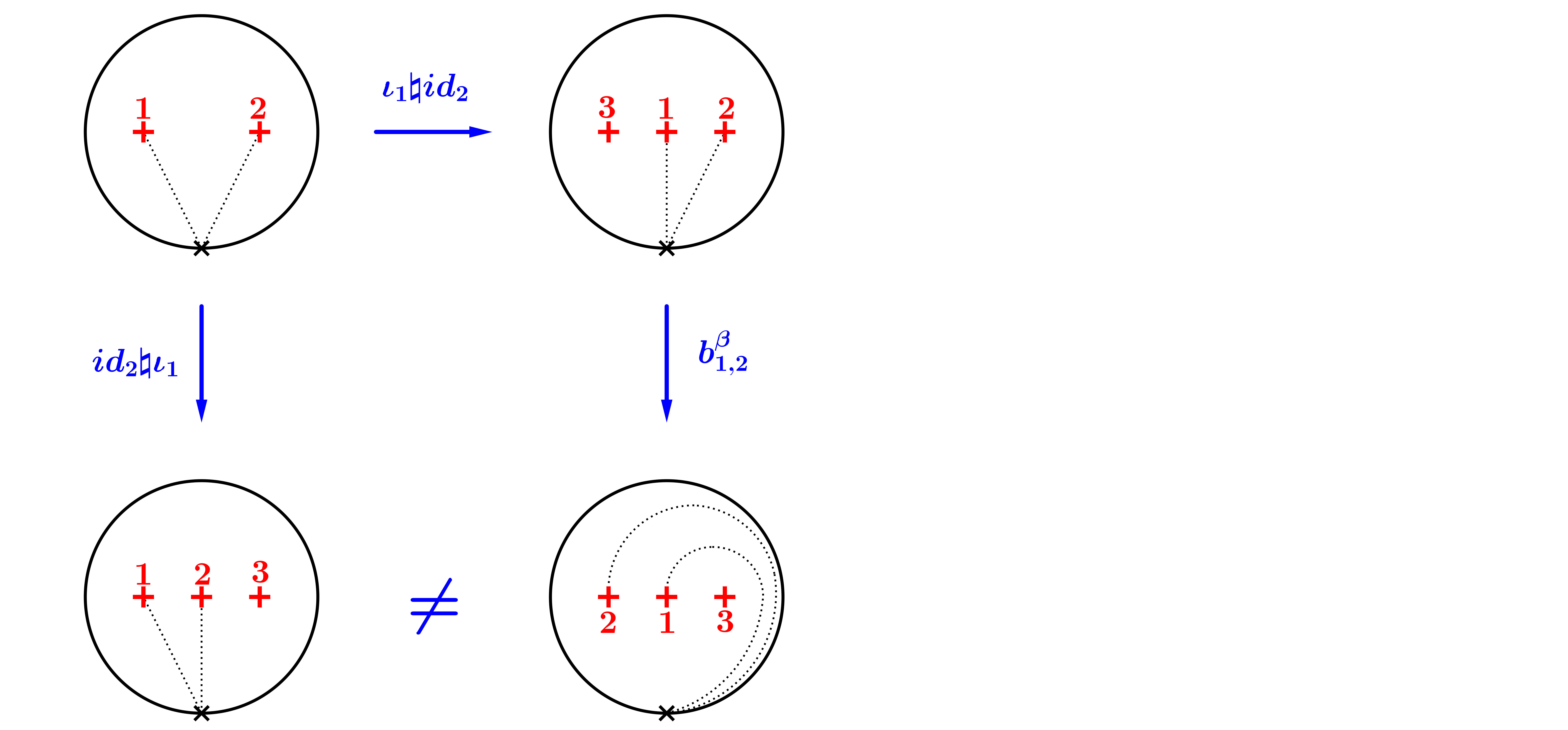 Figure 1