Detecting dynamical changes in time series by using the Jensen Shannon Divergence
D. M. Mateos, L. Riveaud, P. W. Lamberti

TL;DR
This paper introduces methods based on Jensen-Shannon Divergence to detect dynamical changes in time series, effectively distinguishing between chaotic and random signals in both simulated and real data.
Contribution
It proposes novel discretization schemes and detection techniques using Information Theory to identify transitions from chaotic to random regimes in time series.
Findings
High accuracy in detecting dynamical changes
Effective differentiation between chaotic and random signals
Successful application to real-world data
Abstract
Most of the time series in nature are a mixture of signals with deterministic and random dynamics. Thus the distinction between these two characteristics becomes important. Distinguishing between chaotic and aleatory signals is difficult because they have a common wide-band power spectrum, a delta-like autocorrelation function, and share other features as well. In general signals are presented as continuous records and require to be discretized for being analyzed. In this work we present different schemes for discretizing and for detection of dynamical changes in time series. One of the main motivations is to detect transition from chaotic regime to random regime. The tools used are originated in Information Theory. The schemes proposed are applied to simulated and real life signals, showing in all cases a high proficiency for detecting changes in the dynamics of the associated time…
Click any figure to enlarge with its caption.
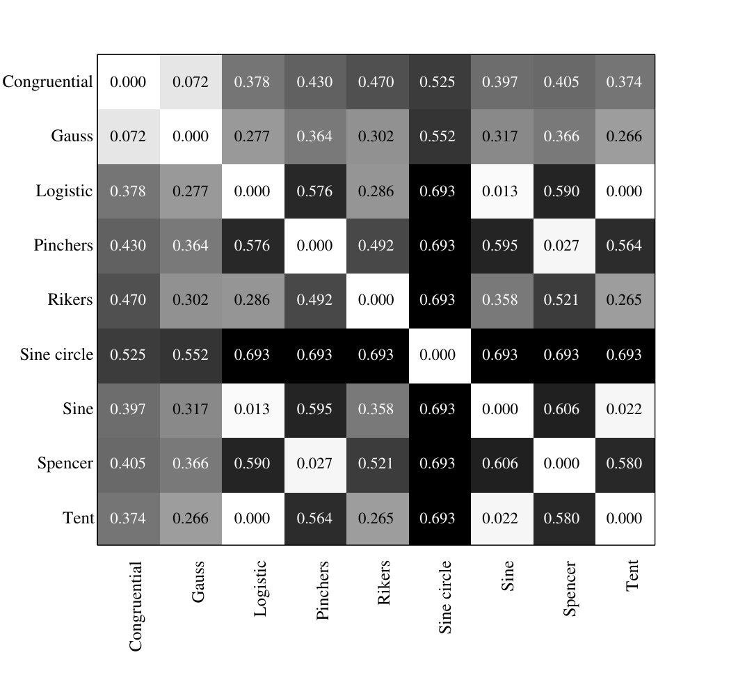 Figure 1
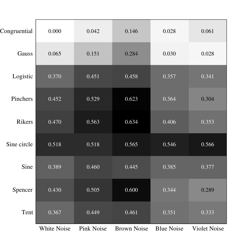 Figure 2
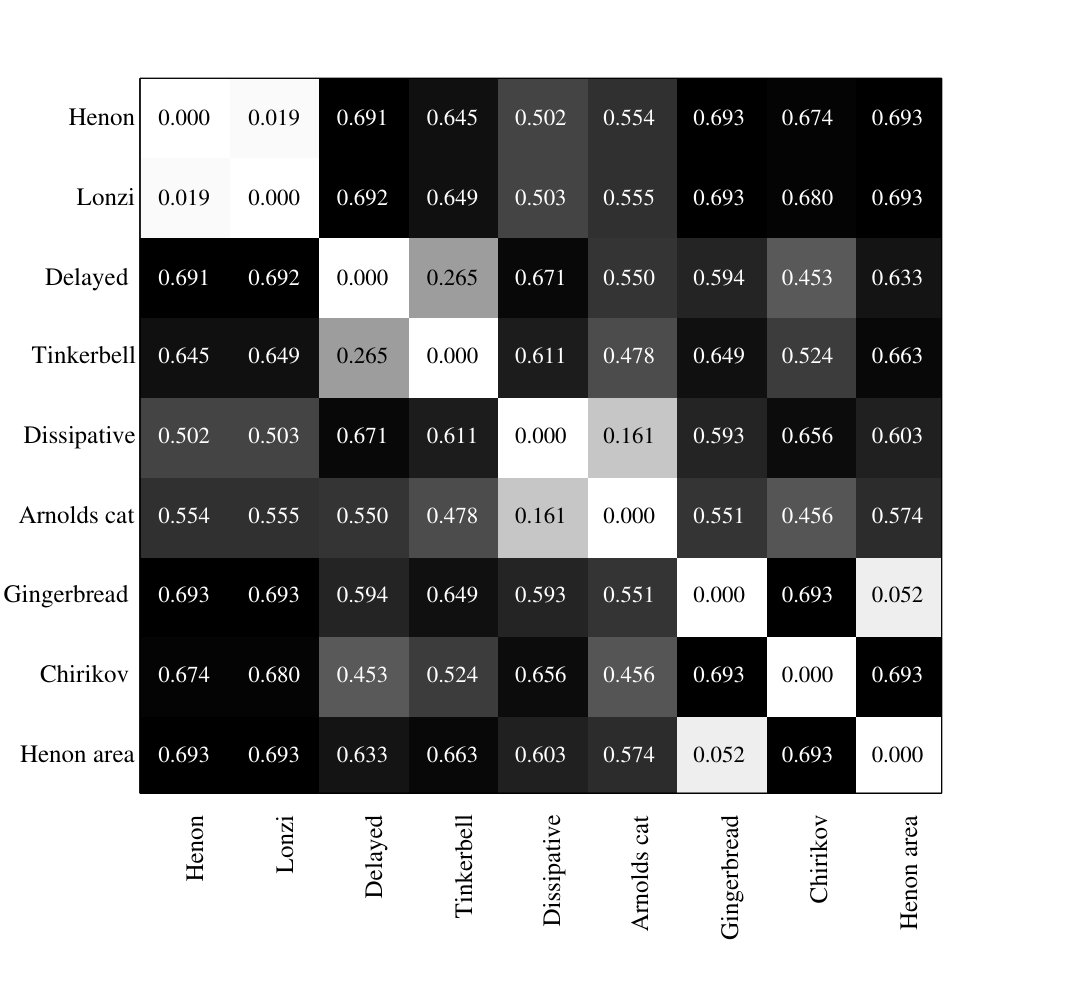 Figure 3
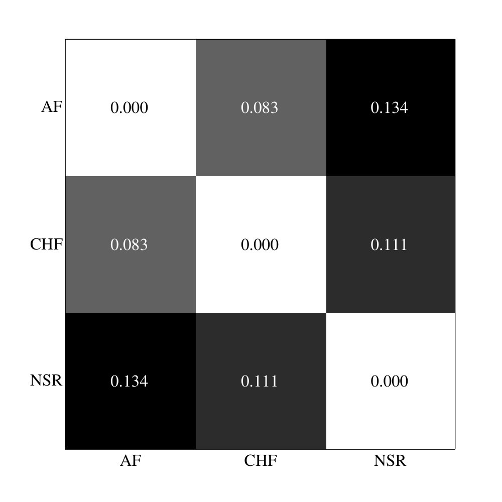 Figure 4
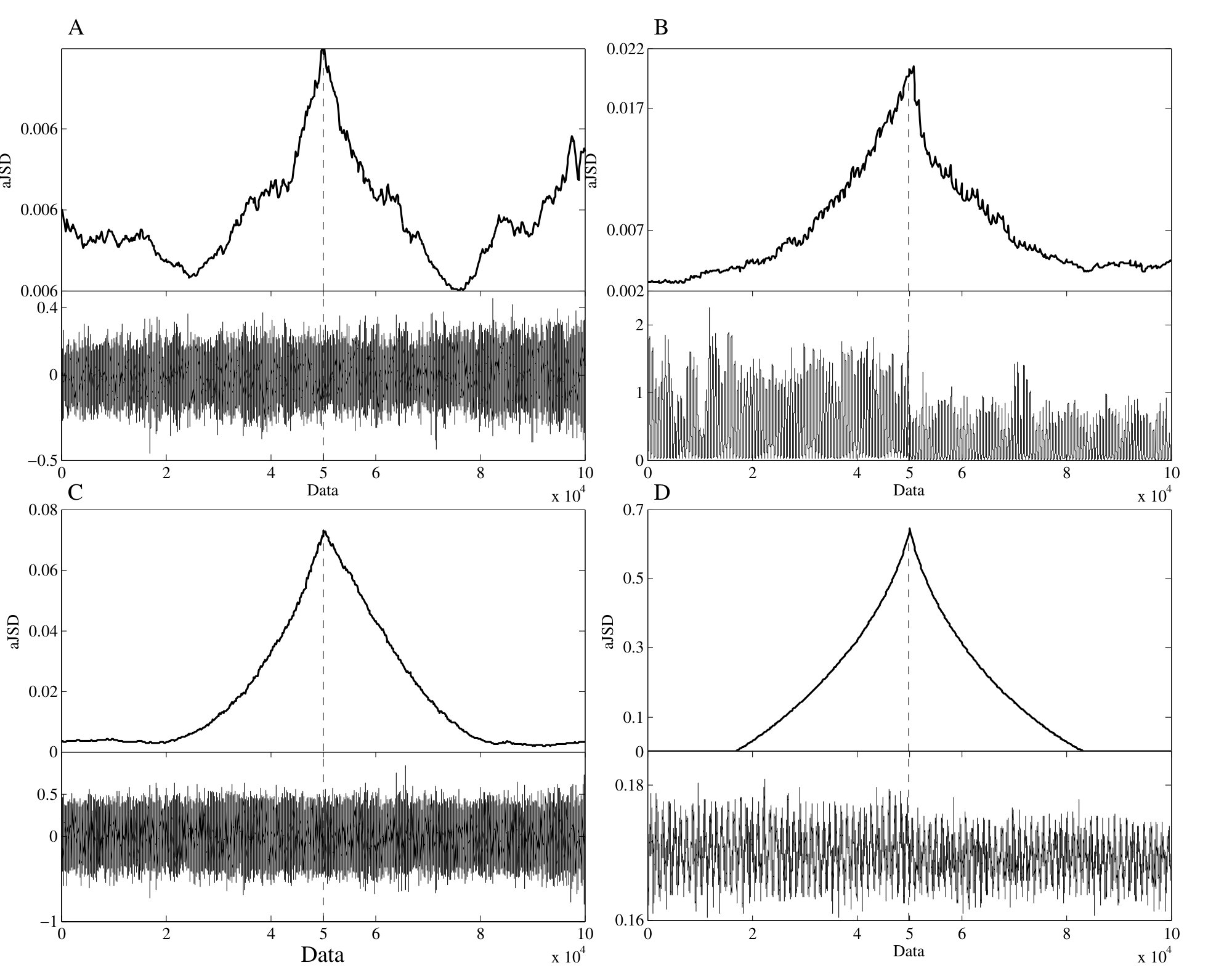 Figure 5
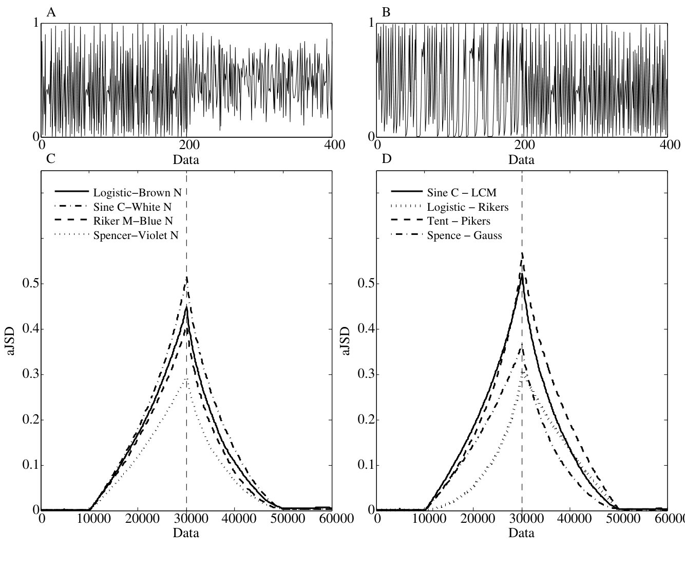 Figure 6
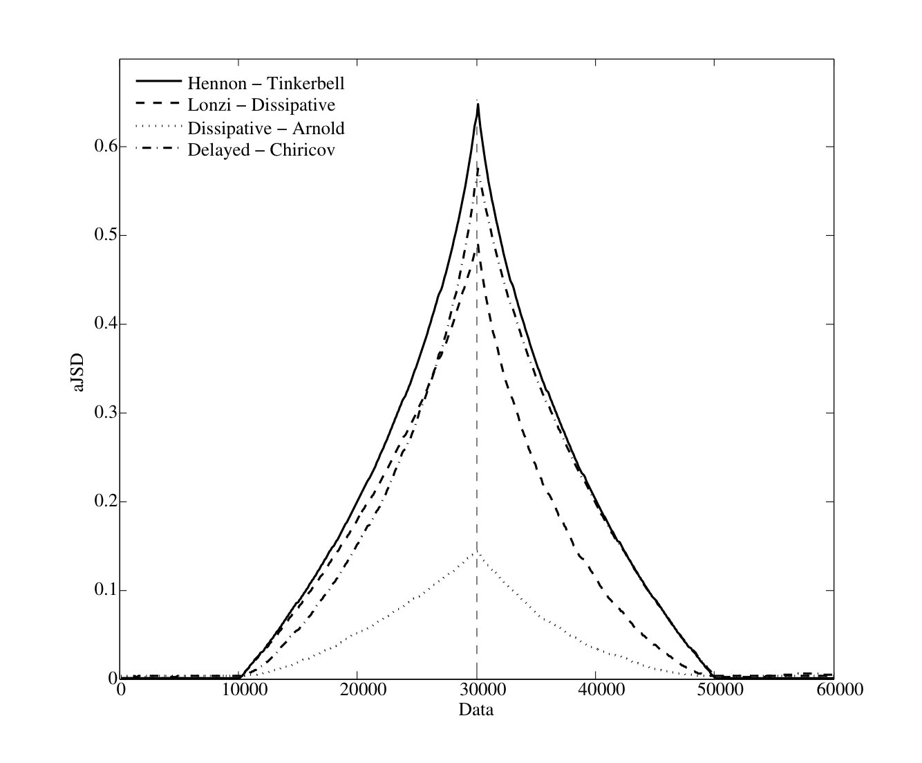 Figure 7
Peer Reviews
No public reviews on file for this paper yet. If you reviewed it on a platform where reviews are public (OpenReview, ICLR, NeurIPS, ICML), you can paste yours below so the community can read it here.
Videos
No videos yet. Explain this paper in a talk, walkthrough, or lecture? Add one.
Detecting dynamical changes in time series by using the Jensen Shannon Divergence
D. M. Mateos1, L. Riveaud2, P. W. Lamberti2
1 Neuroscience and Mental Health Programme, Division of Neurology, Hospital for Sick Children.
Institute of Medical Science and Department of Paediatrics, University of Toronto, Toronto, Canada.
2 Facultad de Matemática, Astronomía, Física y Computación (FaMAF), CONICET, and Universidad Nacional de Córdoba, Córdoba, Argentina
Abstract
Most of the time series in nature are a mixture of signals with deterministic and random dynamics. Thus the distinction between these two characteristics becomes important. Distinguishing between chaotic and aleatory signals is difficult because they have a common wide-band power spectrum, a delta-like autocorrelation function, and share other features as well. In general signals are presented as continuous records and require to be discretized for being analyzed. In this work we present different schemes for discretizing and for detection of dynamical changes in time series. One of the main motivations is to detect transition from chaotic regime to random regime. The tools used are originated in Information Theory. The schemes proposed are applied to simulated and real life signals, showing in all cases a high proficiency for detecting changes in the dynamics of the associated time series.
1 Introduction
In many areas of science the dynamics of processes underlying the studied phenomena can be represented by means of finite time series, that can be interpreted as realizations of stochastic processes (SP) or as orbits of deterministic processes. Although they are very different in nature, Wold demonstrated that under certain restrictions there is a relationship between them [1]. His famous theorem establishes that a stationary stochastic process can be decomposed as a deterministic part (DP), which can be described accurately by a linear combination of its own past, and a second part represented as moving average component of finite order. A different situation occurs when we have a non stationary time series. In these situations it is not possible to separate the series in a deterministic and in a stochastic part. Moreover, in cases in which the DP is chaotic, it is possible to find a DP which produces a time series that could be very difficult to distinguish of a SP [2, 3]. For these reasons, the issue of distinguishing between time series produced by deterministic chaos from noise has led to the development of different scheme of analysis. This problem has already been treated with various techniques such as: complexity-entropy plane [4, 5, 6], Lyapunov exponents [7, 2, 8] or applying neural networks [9], among others. Chaotic signals always produce time series with strong physical structure, unlike those originated in stochastic processes. These have a little structure depending on their correlations factors [10]. The basic idea behind our schemes is to use quantifiers of how close or far are two time series. The quantifiers is the Jensen–Shannon Divergence (JSD), which was introduced as a measure of similarity between two probability distributions function (PDF) [11].
Quantifiers based on information theory, such as the JSD require to associate to a given time series a probability distribution (PD). Thus the determination of the most suitable PD is a fundamental problem, because of the PD and the sample space are inextricably linked. Many methods have been proposed to deal with this problem. Among others, we can mention binary symbolic dynamics [12], Fourier analysis [13], frequency counting [14], wavelet transform [15] or comparing the order of neighboring relative values [16]. In a similar approach, we propose to explore a way of mapping continuous-state sequences into discrete-state sequences via the so-called alphabetic mapping [17].
Here we present two methods for analyzing time series. The first one provides a relative distance between two different time series. It consists in the application of the JSD to a previously discretized signal, through alphabetic mapping. The quantity so evaluated will be called the alphabetic Jensen–Shannon divergence (aJSD). The second method detects the changes in the dynamics of a time series, through an sliding window which run over the previously mapped signal. This window is divided in two parts. To each part we can assign the corresponding PD, which can be compared by using the JSD. In both cases the change in the underlying dynamics of the time series can be detected by analyzing the changes in the value of the JSD at the neighborhood of the time when the change occurs. Both methods were tested by using well known chaotic and random signals taken from the literature and biophysical and mechanical real signals.
The structure of this work is the following: In section 2 we give a brief introduction of the Jensen Shannon divergence, and we explained in detail the alphabetic mapping. In section 3 we introduce the aJSD. In section 4 we give a brief characterization of the chaotic maps and colored noises. We display the analysis of the chaotic and noisy series in section 5. In section 6 we illustrate how the alphabetic Jensen Shannon divergence can be used for real data extracted from biological and mechanical systems. We finish the paper by drawing up some conclusions.
2 Jensen-Shannon divergence for alphabetic mapping
2.1 Jensen-Shannon Divergence
The Jensen Shannon divergence (JSD) is a distance measure between probability distributions introduced by C. Rao [18] and J. Lin [19] as a symmetric version of the Kullback–Leibler divergence. I. Grosse and co-workers improved a recursive segmentation algorithm for symbolic sequences based on the JSD [20].
Let be a discrete-states variable , and let and be two probability distributions for , which we denote as and , with and for all and . If and denote the weights of and respectively, with the restrictions and , the JSD is defined by
[TABLE]
where
[TABLE]
is the Shannon entropy for the probability distribution . We take so that the entropy (and also the JSD) is measured in bits.
It can be shown that the JSD is positive defined, symmetric and it is zero if and only if [11]. Moreover JSD is always well defined, it is the square of a metric [21] and it can be generalized to compare an arbitrary number of distributions, in the following way: Let be a set of probability distributions and let be a collection of non negative numbers such that . Then the JSD between the probability distributions with is defined by
[TABLE]
2.2 Alphabetic Mapping
In Nature it can be found discrete-state sequences, such as DNA sequences or those generated by logical circuits, but most of the “ the real life” signals are presented as continuous records. Thus to use the JSD first we have to discrete the data 111 It is possible to calculate entropy for continuous states signals but the estimation of a differential entropy from the data is not an easy task [22]. . There are many ways to overcome this requirement. Here we use the alphabetic mapping introduced by Yang [17].
For a given continuous series , we can mapping this real-values series in a binary series easily, depending the relative values between two neighbor points in the following way:
[TABLE]
is a binary sequence where or . Consider two integers and , let us then define a trajectory in the -dimensional space as
[TABLE]
The vector is called “alphabetic word´´, where is the “embedding dimension´´ (the number of bit taken to create the word) and is called the ”delay”. Taken’s theorem gives conditions on and , such that preserves the dynamical properties of the full dynamic system (e.g, reconstruction of strange attractors) [23, 24].
By shifting one data point at time, the algorithm produces a collection of bit-word over the whole series. Therefore, it is plausible that the occurrence of these bit-word reflects the underlying dynamics of the original time series. Different types of dynamics produce different distributions on these series. We define , as the symbol corresponding to the word . From these we construct a new series which quantify the original series. The number of the different symbols (alphabet length) depends on the number of bit taken; in this case is .
To give an example of the mapping we can consider the series , which has a corresponding the serie . For the election of the parameter and , the first word to appear is , the second one is , and the other three are , and .
Frequently it is necessary to process signals of two or more dimensions such as bi-dimensional chaotic maps, polysomnography, EEG, etc. The components of such signals are mostly coupled, given signal values depending not only on the previous values but also on the values reached by the other signals. Therefore by making a one-dimensional analysis we can lost some valuable information. Taking the idea discussed above for one-dimensional signals (1D), we have applied the same algorithm with a slight modification to analyze 2-dimensional (2D) signals without loosing information.
For a given continuous 2D series , we assign a 1D string, by the relative values between the two components vector at each time , in the following way:
[TABLE]
3 JSD combined with the alphabetic mapping
Once discretized the signals we can approximate the PD by the frequency of occurrence of the symbols . From this PD, we can develop the following analysis schemes:
- •
Distance between two signals: Given two different sequences, for example, a chaotic and a random sequences, we map each one by using the methodos explained in section 2.2. This gives us two sets of symbols and . We calculate the frequency appearance of the symbols for both sequences and . Finally, we calculate the Jensen Shannon divergence between these two distributions .
- •
Sliding Window: We introduce an sliding window that moves over the symbolic sequence corresponding to the original signal. The window has a width and the position (referring the position of the center of the window over the sequence). For each position , we can divide the window in two sub windows, one to the left and the other to the right of the position . For both windows, we evaluate the frequency of occurrence of symbolic patterns: to the right and to the left . Finally we evaluate the associate JSD, as a function of the pointer position . The position where the maximum value of the JSD occurs, , it is interpreted as the place where a significant change in the probability distribution patterns , has occurred. This change can be associated to a variation in the statistical properties of the original signal. The only restriction in the election of window’s width is that must be greater than the number of possible patterns generated by the alphabetic mapping .
Two sequences with the same statistical properties, should lead to identical probability distributions and therefore, the divergence between them should take a very small value, close to zero but non zero. This fact is due to the statistical fluctuations. The estimators for probability distributions corresponding to sequences must be constructed and then the fluctuations of this construction will yield to JSD values greater than zero. To address this problem Grosse et al. [20] introduced a quantity called ”significance” which allows to see if the values reached by the JSD are greater than the statistical fluctuations. This amount depends on the sequence length and the size of the alphabet of symbols used in the representation of the sequence. An expression for the significance value has presented in the reference [20]. A limitation of that expression is that it is valid only for an alphabet with no more than five symbols. Therefore we must modify the criteria introduced by Grosse et al, to identify values of the JSD that are genuinely above statistical fluctuations. To do that, we proposed to calculate the aJSD on a set of ensembles generated for each signal using the same parameters but with different initial conditions. After quantifying the signals we have differents sequences .
The first step is to calculate the aJSD between all sequences belonging to the same group of segments, that we call “auto-aJSD´´,
[TABLE]
Then we evaluate the average value over all the sets of sequences with its respective standard deviation (). The next step is the same, but using the two group of signals to be compared. For all the aJSD values resulting from all the signal we take the average , with its respective standard deviation ().
Finally two sequences are different (in the statistical sense) if the inequality:
[TABLE]
is satisfied. If the values of the aJSD do not pass this criteria we say that the two signals are not statistically distinguishable one from each other.
4 Characterization of chaotic maps and colored noises
To test our scheme of analysis we used sequences extracted from the bibliography. We use 18 chaotic maps and 5 colored noises, that we describe briefly.
4.1 Chaotic maps
We consider 18 chaotic maps which were taken from the reference [25]. They can be grouped as follows:
1D chaotic maps: also call non–inverted maps. They are dynamical sequences for wich the image has more than one pre-image and in each interaction a loss of information occurs, generating in this way a chaotic system [25].
- •
the lineal congruential generator [26],
- •
the gaussian map [27],
- •
the logistic map [28],
- •
the Pinchers map [29],
- •
the Ricker’s population model [30],
- •
the sine circle [31],
- •
the sine map [32],
- •
the Spencer map [33] and
- •
the tent map [34].
The maps that have been used are :
- •
the Hénon map [35],
- •
the Lonzi map,
- •
the delayed logistic map [36],
- •
the tinkerbell map [37],
- •
the dissipative standard map [38],
- •
the Arnold’s cat map [39],
- •
the chaotic web map [40],
- •
the Chirikov standard map [41],
- •
the gingerbreadman map [42] and
- •
the Hénon area-preserving quadratic map [35].
4.2 Colored noises
Noises with a power spectrum that varies with frequency are called colored noises. There are many types of noises, depending on the shape of the power spectrum and the distribution of values. The noise power spectrum often varies with frequency as (some time called Hurst noise). White noise correspond to . To generate all noises we used the algorithm described in [4, 43]
5 Distinguishing between chaotic and random sequences
In this section we present the results obtained from evaluating the aJSD between chaotic maps and colored noises. We apply the two methods described in section 2. First we create an aJSD distance matrix between chaotic and noise signals and between chaotic and chaotic maps. In the second place we merge two different signals (i.e. one chaotic and one noisy) and through the aJSD sliding window method it is possible to detect the signal changes from one regime to another.
5.1 Distance matrix between sequences
For each type of process explained in the previous section we generate time series of data points with identical parameters [25] and a random initialation. We compute a distances matrix between chaotic and colored noises, using the significance criterion for the aJSD values as explained in section 3. For the discretization of the signals we used the parameters and . Fig. 1 displays the matrix for the corresponding parameters and . For different embedding dimension, we obtained similar results.
In the case of the aJSD distances matrix corresponding to chaos-noise (Fig: 1) we can observe that most of chaotic maps are distinguishable from the different types of colorated noises. The number in the boxes represent the values of the aJSD. Lower is this value, more similar are the sequences.
Only for the particular case of the lineal congruential generator map (LCG) and white noise (WN), the aJSD value does not pass the significance criterion. An interpretation of this is that the LCG map is an example of a random number generator passing the Miller–Rabin test [44]. Therefore the distribution of words corresponding to LCG and WN are similar.
The same evaluation have been done between chaotic maps. Figure 2 displays the corresponding distance matrix. As it can be seen all the aJSD values are above significance criterion, showing our method to be adequated to distinguish between different types of chaos. A more detailed analysis shows a strong relationship between the values of aJSD and the phase diagram of the chaotic maps. For example, the logistic map and the tent map have similar phase diagrams 222 All phase diagrams belong to chaotic time series used in this work are shown in the Sprott book (Apendix [25]), and the value of the distance between both sequences is very low. The same behaviour can be found between the Pincher’s map and the Spencer map.
The same analysis was performed for 2D chaotic series. In this case we use the two-dimensional assignment described in section 2.2 and where the parameters and were chosen . Fig 3 shows the corresponding aJSD distance matrix for the parameters and . As observed for one-dimensional chaotic maps, all distances over passed the significance criteria, being all maps distinguishable one from each other. There exists an strong correspondence between the values of the aJSD and the similarity (or dissimilarity) of the topology of the phase diagrams of the maps. The aJSD values decrease as the topology of the phase diagram tend to be similar, can see it in the case of Hénon map and the Lonzi map. Conversely when two maps are topographical different, such Hénon map preserver area and Chirikov map, the aJSD increas. Different embedding dimensions changes the absolute value of the aJSD but the relative value between the elements of the distance matrix remain unaltered.
Let us recall that in our scheme the aJSD measure the distance between the PDF associated with the set of words and . As a consequence of the Taken’s theorem [24], these sets of words are in correspondence with certain aspects of the phase space of each original signal. Series which have a similar dynamics, have similar phase space and PDF comparable giving low values of the aJSD.
5.2 Detection changes in time series
Here we use the proposed sliding window scheme for detecting changes in a signal. For this purpose we used two different signals of equal length symbols each one, which are merged in a single sequence, where the signal is a chaotic one and is a random one, or two different chaotic sequences. Examples of two combined normalized sequences are plotted in Figures. 4 A and B. Figure 4 shows the results obtained by applying the aJSD to four combinations of chaos-noise sequences. The aJSD achieves its maximum value exactly at the merging point of the two sequences, which is marked with a dotted vertical line. Similar results were observed in the case of sequences generated by chaotic processes. In these cases the aJSD value reaches several orders of magnitude higher than those corresponding to a single stationary sequence.
6 Application of the aJSD to real data
Now we test our proposed schemes for a group of real world signals. The first one is a set of ECG signals on which we calculated the distance matrix of aJSD between groups of patients with different cardiac pathologies. In the second application we use our methods to detected the alignment of the axis of an electric motor.
6.1 Distinction between groups of patients with heart diseases
In this study case the signals correspond to the time intervals between heartbeats (BBI) on 15 patients. The patients were grouped into 3 set of 5 patients each one. The first group consists of healthy persons with normal sinus rhythm (NSR); the second set contains patients suffering from congestive heart failure (CHF), and the third one is composed of patients suffering atrial fibrillation (AF). These set of data are freely available at: www.physionet.org/challenge/chaos/.
Each series represents a record of 24 hours (approximately 100,000 intervals). The analysed records do not have any previous filter. Figure 5 plots the aJSD distance matrix among the three sets, for the parameters ( and ). The aJSD can discriminate between the members of the control group and the pathological groups, being greater the distance between the members of the pathological groups and the members of the control group. The frequency time between heartbeats for the patients belonging to the control group, remains virtually unchanged, while for patients with pathologies the interbeats time is altered. The difference between heartbeats is captured through the alphabetical mapping, giving different patterns distributions of for each group.
6.2 Misalignment detection of an electric motor
The second example corresponds to a record taken from the axis movement of an electric motor. The first signal corresponds to the vibration measure using a capacitive accelerometer, mounted along the axis on the motor bearing (Figure 6A). The second one, is a signal taken from an optical incremental rotary encoder drum, with about 145 pulses per revolution as shown in Figure ( 6B). The third is a signal generated by a piezoelectric accelerometer mounted in the same place that the capacitive signal, which is plotted in Figure ( 6C). The last signal is the rate of the engine load and depicted in Figure (6D) 333It is related to the frequency of rotation of the shaft by means of a ”Keyphaser” . The data were obtained with a sampling frequency of Hz without any preprocessing. For more technical details on the recording setup see (reference [45])
Each signal has a length of , in where the first measurement values correspond to axis in the aligned position and the in misaligned position. For all the signals we used the following parameters: , and . The results are shown in Fig. 6. It should be noted that for all signals, the aJSD maximum value is reached exactly when the shaft alignment state changes. That point is identified by the dotted vertical line. In the case of the signals from the vibration measurement by the piezoelectric accelerometers as capacitive, the value of the maximum aJSD is smaller and more volatile than the other two methods. This fact can be associated with the efficacy of the measurement method. In all cases the different signals are clearly detectable by the methods here proposed.
7 Discussion
In paper we have introduced the notion of alphabetic Jensen Shannon Divergence to measure a the distance between time series. The method can be used for one-dimensional and two-dimensional signals. Using this measure, we have developed two methods to distinguish between different types of signals. Particularly we used them distinguish random from chaotic signals, and to compare different types of chaotic signals between them. Through the aJSD distance matrix, we were able to show that chaotic signals are clearly distinguishable from random signals with diverse power spectrum. It is important to remark that chaotic signals with different phase space structure are distinguishable from one another, also. The values taken by the entries of the distance matrix, are in correspond with the similarity (or dissimilarity of the corresponding phase spaces). This fact was observed for one and two dimensional chaotic sequences. Our methods were also applied to real world sequences. In particular some corresponding to ECG records, from healthy and sick patients.
We also developed a procedure detect dynamical changes in a signal by using a sliding window that moves on the resulting symbolic sequence after mapping the original series by a alphabetical assignment, being the centre of the original window moved a place per step. Then the aJSD is evaluated for the two corresponding sub-sequences belonging to each half of the window. The maximum value of the divergence corresponds to the point where occurs a change in the probability distribution of the discretized signal. We tested the method using two different signals merged. The aJSD allows to detect the point where the two different signals were coupled in order to constitute signals with chaos-noise and chaos-chaos parts. Finally we use this scheme to evaluate the alignment condition of the axis of an electric motor.
Both methods have shown to be robust respect to the election of the parameters in the probability distribution evaluation. Among the main advantage we can highlight that both are easily implemented for the analysis of real world signals.
Acknowledgments
The authors thank Dr. Pierre Granjon from the GIPSA-lab, Grenoble, France, for kindly providing them with the recording electric motor data and Consejo Nacional de Investigaciones Científicas y Técnicas (CONICET) for financial assistance. They also thank Dr. Jose Luis Perez–Velazquez for useful discussions.
The reference list from the paper itself. Each links out to its DOI / PubMed record.
- 1[1] H. Wold. A study in the analysis of stationary time series . Almqvist & Wiksell, 1938.
- 2[2] M. Cencini, M. Falcioni, E. Olbrich, H. Kantz, and A. Vulpiani. Chaos or noise: Difficulties of a distinction. Physical Review E , 62(1):427, 2000.
- 3[3] H. Sakai and H. Tokumaru. Autocorrelations of a certain chaos. Acoustics, Speech and Signal Processing, IEEE Transactions on , 28(5):588–590, 1980.
- 4[4] O. A. Rosso, H. A. Larrondo, M. T. Martin, A. Plastino, and M. A. Fuentes. Distinguishing noise from chaos. Physical review letters , 99(15):154102, 2007.
- 5[5] L. Zunino, M. C. Soriano, and O. A Rosso. Distinguishing chaotic and stochastic dynamics from time series by using a multiscale symbolic approach. Physical Review E , 86(4):046210, 2012.
- 6[6] F. Olivares, A. Plastino, and O. A. Rosso. Contrasting chaos with noise via local versus global information quantifiers. Physics Letters A , 376(19):1577–1583, 2012.
- 7[7] W. A. Brock. Distinguishing random and deterministic systems: Abridged version. Journal of Economic Theory , 40(1):168–195, 1986.
- 8[8] J. B. Gao, J. Hu, W. W. Tung, and Y. H. Cao. Distinguishing chaos from noise by scale-dependent lyapunov exponent. Physical Review E , 74(6):066204, 2006.