Local recovery of the compressional and shear speeds from the hyperbolic DN map
Plamen Stefanov, Gunther Uhlmann, Andras vasy

TL;DR
This paper demonstrates that local boundary measurements can uniquely determine the compressional and shear wave speeds in an elastic medium, given certain geometric conditions, advancing inverse boundary value problem theory.
Contribution
It establishes unique local recovery of elastic wave speeds from boundary data under convex foliation conditions, a novel result in inverse elastic problems.
Findings
Local boundary data determines p-wave speed with convex foliation.
Local boundary data determines s-wave speed with convex foliation.
Unique determination of wave speeds from boundary measurements.
Abstract
We study the isotropic elastic wave equation in a bounded domain with boundary. We show that local knowledge of the Dirichlet-to-Neumann map determines uniquely the speed of the p-wave locally if there is a strictly convex foliation with respect to it, and similarly for the s-wave speed.
Click any figure to enlarge with its caption.
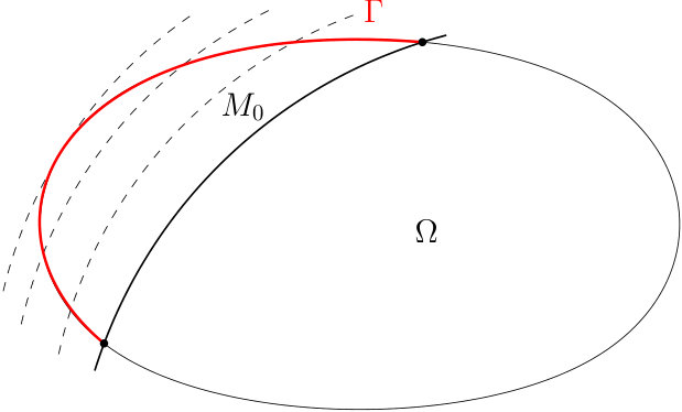 Figure 1
Peer Reviews
No public reviews on file for this paper yet. If you reviewed it on a platform where reviews are public (OpenReview, ICLR, NeurIPS, ICML), you can paste yours below so the community can read it here.
Videos
No videos yet. Explain this paper in a talk, walkthrough, or lecture? Add one.
Local recovery of the compressional and shear speeds from the hyperbolic DN map
Plamen Stefanov
Department of Mathematics, Purdue University, West Lafayette, IN 47907
,
Gunther Uhlmann
Department of Mathematics, University of Washington, Seattle, WA 98195, Department of Mathematics University of Helsinki, Finland, IAS, HKUST, Clear Water Bay, Hong Kong, China
and
Andras Vasy
Department of Mathematics, Stanford University, Stanford CA 94305
Abstract.
We study the isotropic elastic wave equation in a bounded domain with boundary. We show that local knowledge of the Dirichlet-to-Neumann map determines uniquely the speed of the p-wave locally if there is a strictly convex foliation with respect to it, and similarly for the s-wave speed.
The authors were partially supported by the National Science Foundation under grant DMS-1600327 (P.S.), DMS-1265958 (G.U.) and DMS-1361432 (A.V.).
1. Introduction
Consider the isotropic elastic wave equation in a smooth bounded domain . We study the following problem: can we determine the Lamé parameters , and the density from the knowledge of the Dirichlet-to-Neumann (DN) map on the boundary? In fact, we are interested in the local problem: local recovery of those parameters from local or even microlocal information about . Our main motivation is the local seismology problem of recovery of the inner structure of the Earth from local measurements on its surface of seismic waves.
This problem is well studied for the wave equation related to a Riemannian metric with either full or partial boundary data. It is known that one can recover up to an isometry fixing pointwise [5], using the boundary control method developed by [2]. The latter relies on the unique continuation result of Tataru [27]. We refer to [13] for related results and more references. Logarithmic type of stability is proved in [7, 14]. Hölder type of stability estimates with full data have been proven in [23, 17, 6, 1] and most recently in [26], under some assumptions on the metric, for example absence of conjugate points.
In the elastic case, the results are less complete. Unique continuation holds [10] but the boundary control method is not known to work, see, e.g., [4]. The reason is that it is not possible, or at least not known how to decouple the elasticity system completely even though it is easy to do that on the principal symbol level or even for the full symbol, see (22) below, but only microlocally. A Lamé type of system having the same principal part which can be decoupled fully was studied in [3] and the boundary control method was used for it for a unique recovery of the two wave speeds locally with a local data. Numerical reconstruction is proposed in [15].
Rachelle [18] proved that one can recover the jet of , and at explicitly. In [19, 20], she showed that one can recover those three parameters in provided that is known on the whole boundary and assuming that the two wave speeds are simple (strict convexity and no conjugate points). The proof is based on recovering the lens relations related to the two speeds and then applying known rigidity results. The recovery of all the three parameters in [20] requires the study of the second order term and an inversion of the geodesic ray transform. The second author and Hansen [11] studied this problem with a residual stress and without the assumption of no-conjugate points or caustics and showed that one can recover both lens relations and derive several consequences of that.
In this work we show that one can recover uniquely the two wave speeds and locally under the assumption of existence of a strictly convex foliation. This condition allows for conjugate points, see, e.g., [16]. If is a ball and the speeds increase when the distance to the center decreases (typical for geophysical applications), the foliation condition is satisfied, see section 6. To prove the main result, we show that one can recover the lens relations related to the two speeds in an explicit way and then apply the results of the authors [24], see also [25], about local recovery of a sound speed in the acoustic equation from the associated lens relation, also known locally. That argument also implies stability as a consequence of the stability result in [24] but we do not make this formal. Also, we can apply the result if there is an internal closed strictly convex surface where the coefficients jump, like in the elastic Earth model, and recover the two speeds between the boundary and that surface. Indeed, for that we only need the lens relation along geodesics not hitting that surface; and that can be extracted from the microlocal support of the DN map. Note that this recovers two quantities depending on the three parameters , and . Recovery of all three parameters would require an analysis of the next order term in the geometric optics construction, similarly to what is done in [20].
2. Main Result
The isotropic elastic system in a smooth bounded domain is described as follows. The elasticity tensor is defined by
[TABLE]
where , are the Lamé parameters. The elastic wave operator is given by
[TABLE]
where is the density and the vector function is the displacement.
The operator is symmetric on . It has has a principal symbol
[TABLE]
Taking and , we recover the well known fact that that has eigenvalues
[TABLE]
of multiplicities and , respectively and eigenspaces , and . Those are known as the speeds of the p-waves and the s-waves, respectively. The eigenspaces correspond to the polarization of those waves. The characteristic variety is the union of and , each one having two connected components (away from the zero section), determined by the sign of .
Let solve the elastic wave equation
[TABLE]
with given so that for . The Dirichlet-to-Neumann map is defined by
[TABLE]
where is the outer unit normal on , and is the stress tensor
[TABLE]
Note that , where is the divergence of the 2-tensor .
Let be an open domain containing and extend the coefficients there in a smooth way.
Definition 1**.**
Let be a smooth function which level sets , , restricted to , are strictly convex viewed from w.r.t. ; on these level sets, , and . Then we call a strictly convex foliation of w.r.t. .
A special case is when is strictly convex w.r.t. and .
We introduce the lens rigidity problem next. For a compact manifold with a boundary, let the manifolds consist of all vectors with , unit in the metric , and pointing outside/inside . We define the scattering relation
[TABLE]
in the following way: for each , , where are the exit point and direction, if exist, of the maximal unit speed geodesic in the metric , issued from . Let
[TABLE]
be its length, possibly infinite. If , we call non-trapping. The maps together are called lens relation (or lens data).
It is convenient to identify vectors in with their projections on the unit ball bundle ; and similarly for . Then we can view and as maps from to itself; or from to , respectively.
Below, we denote by and the lens relations in w.r.t. the metrics and , respectively. Similarly, we denote the corresponding ’s by and .
Theorem 1**.**
Let , , be smooth in . Let , be a strictly convex foliation w.r.t. , and let . Then for every , is uniquely determined on the foliation by knowledge, up to a smooth function, of the kernel of on , if is greater than the length of all geodesics, in the metric , in having the property that each one is tangent to some of the hypersurfaces in the foliation.
The same statement remains true for replaced by .
We refer to Figure 1 for an illustration of the set where we can recover the speeds.
We only need microlocal information about , wee Remark 5.1. Also, since and are part of the wave front set of the kernel of , we can argue that they can be recovered stably form it; and in fact, they are directly observable in seismic experiments. Then one can apply the stability result in [24] to conclude that and are stably recoverable from . We will not make this statement more precise in this paper.
3. Preliminaries
3.1. An invariant formulation
We have
[TABLE]
This can also be written in the following divergence form.
[TABLE]
where is the symmetric differential, and is the divergence of symmetric fields.
To prepare ourselves for changes of variables needed in the analysis near surfaces that we will flatten out, we will write in invariant way in the presence of a Riemannian metric . We view as an one form (a covector field) and we define the symmetric differential and the divergence by
[TABLE]
where is the covariant differential, , is a covector field, and is a symmetric covariant tensor field of order two. Note that increases the order of the tensor by one while decreases it by one. Then we define by (7). The stress tensor (4) is given by
[TABLE]
and then . The Neumann boundary condition at is still given by prescribing the values of on it as in (3). The operator , defined originally on extends to a self-adjoint operator in . This extension is the one satisfying the zero Dirichlet boundary condition on . In particular, this shows that the mixed problem (2) is solvable with smooth data at least since one can always extend inside and reduce the problem to solving one with a zero boundary condition and a non-zero source term; and then use the Duhamel’s principle for the latter.
We show next that the data on the boundary is equivalent to knowing the Cauchy data on it, see also [18, sec. 3.1]. In next lemma, we use semigeodesic coordinates to a given hypersurface , with on one side of it, defining the orientation. The Euclidean metric then takes the form in those coordinates with for .
Lemma 1**.**
For every hypersurface , the pair determined uniquely the Cauchy data . More precisely, in semigeodesic coordinates, the normal derivative of on can be obtained from and by the relations
[TABLE]
where are the Christoffel symbols of the Euclidean metric in semigeodesic coordinates.
Before presenting the proof, we want to emphasize that is also transformed in the new coordinates (as a covector), and is the divergence w.r.t. the transformed metric. Also, in a more invariant form, (9) takes the form
[TABLE]
where is the covariant derivative, and we used the fact that .
Proof.
In those coordinates,
[TABLE]
Setting , we get the second formula in (9) because . Taking , we get the first one one. ∎
4. Geometric optics for the elastic wave equation
We recall the well known geometric optics construction for the acoustic and the elastic wave equations, see, e.g., [28, 29].
4.1. The Cauchy Problem with data at in the acoustic case
We start with the scalar acoustic case which we use in the analysis of the elastic one. We work in arbitrary dimensions here. Details can be found in [28, 29], for example.
We recall briefly the geometric optic construction for the acoustic wave equation
[TABLE]
with Cauchy data at . Here, is a Riemannian metric that we include in order to have the flexibility to change coordinates easily; and is the Laplace-Beltrami operator. Up to lower order terms, coincides with with . We are looking for solutions of the form
[TABLE]
modulo terms involving smoothing operators of and , defined in some neighborhood of , with some . This parametrix differs from the actual solution by a smoothing operator applied to , as it follows from standard hyperbolic estimates.
Here, are classical amplitudes of order zero depending smoothly on of the form
[TABLE]
where is homogeneous in of degree for large . The phase functions are positively homogeneous of order in solving the eikonal equations
[TABLE]
Such solutions exist locally only, in general.
Equate the order terms in the expansion of to get that the principal terms of the amplitudes must solve the transport equation
[TABLE]
with appropriate initial conditions and
[TABLE]
Equating terms homogeneous in of lower order we get transport equations for , with the same left-hand side as in (15) with a right-hand side determined by .
The transport equations are ODEs along the zero bicharacteristics, which are just the geodesics of the metric lifted to the phase space, with vectors identified by covectors by the metric. The integrals appearing in (12) are Fourier Integral Operators (FIOs) either with considered as a parameter, or as considered as one of the variables. In the former case, singularities of propagate along the zero bicharacteristics. More precisely, for every ,
[TABLE]
where , and
[TABLE]
and for , is the geodesic issued from in direction .
On the other hand, considering as one of the variables,
[TABLE]
where
[TABLE]
In the analysis below, we will consider only.
The construction above can be done in some neighborhood of a fixed point in general. To extend it globally, we can localize it first for with in a conic neighborhood of some fixed . Then will be well defined near the geodesic issued from that point but in some neighborhood of in general. We can fix some at which is still defined, take the Cauchy data there and use it to construct a new solution. Then we get an FIO which is a composition of the two local FIOs each one associated with a canonical diffeomorphism, then so is the composition. Then we can use a partition of unity to conclude that while the representation (12) is local, the conclusions (17) and (18) are global. In fact, it is well known that both and with fixed are global FIOs associated with the canonical relations in (17) and (18).
In particular, if is a smooth hypersurface, and hits for the first time transversely locally, then is an FIO again with a canonical relation as above but with and replaced by its tangential projection . Notice that for and for . Also, with equality for tangent rays which we exclude.
4.2. The Cauchy problem at and propagation of singularities in the elastic case
We consider the elastic system in now. Actually, most of the analysis holds for arbitrary but since we rely on the analysis of the principal symbol of below done in three dimensions, we consider . Since the characteristics are of constant multiplicities, this case is well understood, see, e.g., [28] that we review below, or [8]. Below we give some details specific for the elastic case which allow us to describe explicitly the boundary data generating p-waves or s-waves only, up to lower order terms.
Consider the elastic wave equation
[TABLE]
with Cauchy data at . We want to solve it microlocally for in some interval and in an open set. Let be the projection to the p-modes, i.e., is the Fourier multiplier and let . It is easy to see that is the Fourier multiplier . Also, we may regard as the potential/solenoidal (or the Hodge) decomposition of the 1-form , see, e.g., [21].
By (1),
[TABLE]
where is the class of classical DOs of order ; and we will denote by the corresponding symbol class. This shows that to construct the leading singularity of the solution, we need to solve the decoupled system
[TABLE]
Those are two vector valued acoustic equations. The singularities propagate along unit speed geodesics lifted to the tangent bundle (identified with the covector one for each speed) of the metrics and , respectively. To relate (21) to (19), set , . Then , where is a DO of order . Next, applying to the initial conditions in (19), we get the initial conditions in the first equation in (21). We get a similar conclusion for . Therefore, and solve a system, compare with (21), of the type
[TABLE]
where are DOs of order one. Since propagation of singularities is governed by the principal part of that system only, we prove the claim associated with (21): the leading singularities, say in modulo with a fixed , of can be computed as in (21); and the whole singularities still propagate along the zero bicharacteristics of the speeds and . This is a general conclusion for the solution of the elastic system since locally, we can always take the traces of and to some hyperplane and view the solution as the one with Cauchy data given by those traces.
We recall also the construction in [28], which provides another proof of the propagation of singularities in this case. The principal symbol of has eigenvalues of constant multiplicities. It is well known, see, e.g., [28] that near every , one can decouple the full symbol fully up to symbols of order . In other words, there exist elliptic matrix valued DOs and of order [math] microlocally defined near , so that
[TABLE]
modulo near , where is scalar, and is a matrix symbol, with principal symbols , . In other words, is scalar and is principally scalar. In fact, can be chosen to be unitary with in microlocal sense [22]. As an example, the principal symbol of can be chosen to be
[TABLE]
when . It then follows that microlocally, the elasticity system decouples into the wave equations with or ; the first one scalar, and the second one a system. The first one has as a characteristic manifold, while the second one has . Even though and depend on the microlocal neighborhoods of the characteristic varieties we work in, the wave front sets of , in those neighborhoods, we can apply the propagation of singularities results, or directly the microlocal geometric optics construction used below. Then we conclude that singularities in those neighborhoods propagate along the zero bicharacteristics of and , respectively. This implies a global result, as well. The advantage of this construction is that we can do it to infinite order.
5. Proof of the main results
The following theorem is a local version of the statement that given , we can recover the lens relations and , see [19, 11] for the global version.
Theorem 2**.**
Let be relatively open and let . For , assume that for every with a singular support in , is known on , up to a smooth function. Then the lens relations and are determined uniquely on the open sets of with so that the unit speed geodesic issued from (i.e., unit speed in the direction of ) in the metric , respectively , is transversal at and hits again, transversely, at a point in at a time not exceeding .
Proof.
By [18], the jets of at are uniquely determined by the kernel of known on for any fixed . Since the proof is based on applying to highly oscillatory functions, any smooth addition to that kernel would not change the reconstruction.
Using this, we extend smoothly to some small neighborhood of in the exterior of in a way determined uniquely by the data in the theorem.
Choose (which is characteristic for the Hamiltonian related to ), with and pointing into . Assume that the null bicharacteristic in (actually, ) through is transversal at that point, and hits again transversely at some with . Extend outside the domain on the side of until it hits at some point . If , this short segment will be outside , i.e., , see Figure 2.
Let an outgoing (smooth for in ) microlocal solution in related to , with a wave front set in only, the latter supported in a small conic neighborhood of . This solution can be constructed by choosing suitable Cauchy data at near as explained in the previous section. We think of as a microlocal p-wave propagating along . We cut smoothly so that its support is concentrated near ; call the result . Then and , for near [math].
The trace of on the boundary can be naturally written as , where have wave front sets in small conic neighborhoods of the projection of on , i.e., close to , , where the prime stands for a tangential projection.
Let solve (2) with (i.e., is replaced by zero). The singularities issued from will propagate to the future only and before they hit again, and differ by a smooth function. When they hit , they will reflect at and there will be a possible mode conversion. We are not going to build a parametrix for the reflection. Instead, it is enough to prove that has a non-empty wave from set in a conic neighborhood of .
Let be extended as zero to . Then , where is the delta function on on the boundary, see (3). Assume ; then at , the wave front set of on the plane spanned by and the conormal to the boundary can be only along the conormal, as it follows by the calculus of the wave front sets. In particular, (the phase component of at that point) cannot be in the wave front set of because the latter is in ; and is certainly not conormal, being characteristic. By the propagation of singularities theorem (with a source term having a wave front set away from the microlocal region of interest), each point of must be a singularity for , or none is. This is a contradiction since is singular on in the domain, and non-singular on outside it. Therefore, .
We can take a sequence of ’s as above with shrinking wave fronts sets to (or take with on the radial ray through ) to conclude that determines the p-lens relation at . Since the part of between and is uniquely determined by the data, conclude that is uniquely determined at as well.
To show that determines the lens relation related to the s-waves on , we argue as above. ∎
Remark 5.1**.**
The proof actually shows that we only need to know the wave front set of the kernel of microlocally at only for and similarly for , in order to decide if belongs to the graph of the p-lens relation with an identification of covectors and vectors by the metric . Here, is the image of (recall that is the projection of ) under the bicharacteristic flow until it hits the boundary; and then projected there.
Proof of Theorem 1.
Consider first. By Theorem 2, we can recover the lens relation on the foliation. By [24], this recover in the region covered by the foliation, as claimed. The proof for is the same. ∎
6. The Herglotz and Wieckert & Zoeppritz condition
We formulate generalized version of the Herglotz [12] and Wieckert and Zoeppritz [30] condition on a speed in the ball :
[TABLE]
where , . The original condition in [12, 30] is about radial speeds only. In particular, (23) holds when , i.e., when the speed decreases in depth. This inequality was shown on [24] to be equivalent to the requirement the Euclidean sphere to be strictly convex with respect to . If is flat locally, the convexity condition is that increases with depth. We formulate those two conditions formally in the following.
Lemma 2**.**
(a) The Euclidean spheres , , form a strictly convex foliation in some set with respect to the metric , viewed from the exterior, if and only if (23) holds for such and for in that set.
(b) The Euclidean hyperplanes , form a strictly convex foliation in some set with respect to the metric , viewed from if and only in that set.
Part (a) is proved in [24]. Those two statements are a partial case of the following more general one. Recall that strict convexity of an oriented hypersurface in a Riemannian manifold is defined as a positivity of the second fundamental form; and if that form in non-negative, we will call convex. If the second fundamental form vanishes at some point of , we call this point flat, which is a special case of convex. Under this definition, totally geodesic hypersurfaces are still convex.
Lemma 3**.**
Let the oriented hypersurface be strictly convex w.r.t. the metric at some point . Fix a smooth . Let be the unit normal derivative at pointing to the convex side. If , then is strictly convex w.r.t. the metric at .
If is flat at , then is an if and only if condition for strict convexity.
Proof.
We work in semigeodesic local coordinates near so that is given locally by and the convex side is . We need to show that the second fundamental form related to on hyperplane is positive when that related to is. Denote the Christoffel symbols of by and those of by . Using the relationship between Christoffel symbols of conformal metrics, we get
[TABLE]
On , which implies in particular, the second fundamental form of and on are related by
[TABLE]
where Greek indices run from to and . Therefore, that form is positive if ; and when the form on the right vanishes, then this is an if and only of condition. ∎
Lemma 2(b) then follows from Lemma 3 since the Euclidean hypersurfaces are convex by our definition (they are flat). Using the fact that the Euclidean spheres are strictly convex, we can derive strict convexity in Lemma 2(a) under the weaker condition . One can check directly the the Euclidean spheres are flat for the metric , which implies Lemma 2(a) in its full strength.
Part (b) and Theorem 1 in particular provide uniqueness for the local seismology problem when the surface of the Earth is modeled as the plane in , and the Earth itself is given locally by , under the conditions and , see Figure 3(b). For deeper regions, the spherical model can be used and then condition (23) guarantees existence of a strictly convex foliation. Those conditions are satisfied in the Upper Mantle, at least, according to the popular Preliminary Reference Earth Model (PERM) [9]. In fact, the stronger condition holds, and Figure 3(a) illustrates typical regions where the uniqueness holds.
The reference list from the paper itself. Each links out to its DOI / PubMed record.
- 1[1] G. Bao and H. Zhang. Sensitivity analysis of an inverse problem for the wave equation with caustics. J. Amer. Math. Soc. , 27(4):953–981, 2014.
- 2[2] M. I. Belishev. An approach to multidimensional inverse problems for the wave equation. Dokl. Akad. Nauk SSSR , 297(3):524–527, 1987.
- 3[3] M. I. Belishev. Dynamical inverse problem for a Lamé type system. J. Inverse Ill-Posed Probl. , 14(8):751–766, 2006.
- 4[4] M. I. Belishev. Recent progress in the boundary control method. Inverse Problems , 23(5):R 1–R 67, 2007.
- 5[5] M. I. Belishev and Y. V. Kurylev. To the reconstruction of a Riemannian manifold via its spectral data (BC-method). Comm. Partial Differential Equations , 17(5-6):767–804, 1992. MR 1177292.
- 6[6] M. Bellassoued and D. Dos Santos Ferreira. Stability estimates for the anisotropic wave equation from the Dirichlet-to-Neumann map. Inverse Probl. Imaging , 5(4):745–773, 2011.
- 7[7] R. Bosi, Y. Kurylev, M. Lassas. Stability of the unique continuation for the wave operator via Tataru inequality and applications. J. Diff. Equations 260:6451–6492, 2016.
- 8[8] N. Dencker. On the propagation of polarization sets for systems of real principal type. J. Funct. Anal. , 46(3):351–372, 1982.