Top-quark mass measurement in the all-hadronic $t\bar{t}$ decay channel at $\sqrt{s}$ = 8 TeV with the ATLAS detector
ATLAS Collaboration

TL;DR
This paper measures the top-quark mass in the all-hadronic decay channel using 8 TeV proton-proton collision data from the ATLAS detector, employing a data-driven background model and template fitting techniques.
Contribution
It presents a novel measurement of the top-quark mass in the all-hadronic channel with improved precision using a large data set and a data-driven background modeling approach.
Findings
Top-quark mass measured as 173.72 GeV with combined uncertainty.
Utilized a data-driven method for multi-jet background modeling.
Achieved a precise top-quark mass measurement in the all-hadronic channel.
Abstract
The top-quark mass is measured in the all-hadronic top-antitop quark decay channel using proton-proton collisions at a centre-of-mass energy of = 8 TeV with the ATLAS detector at the CERN Large Hadron Collider. The data set used in the analysis corresponds to an integrated luminosity of 20.2 fb. The large multi-jet background is modelled using a data-driven method. The top-quark mass is obtained from template fits to the ratio of the three-jet to the dijet mass. The three-jet mass is obtained from the three jets assigned to the top quark decay. From these three jets the dijet mass is obtained using the two jets assigned to the W boson decay. The top-quark mass is measured to be 173.72 0.55 (stat.) 1.01 (syst.) GeV.
Click any figure to enlarge with its caption.
 Figure 1
 Figure 2
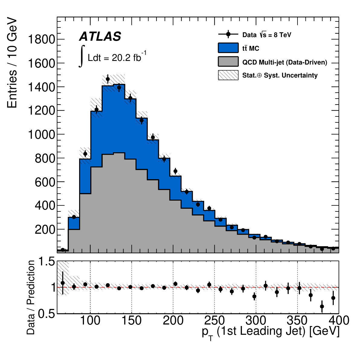 Figure 3
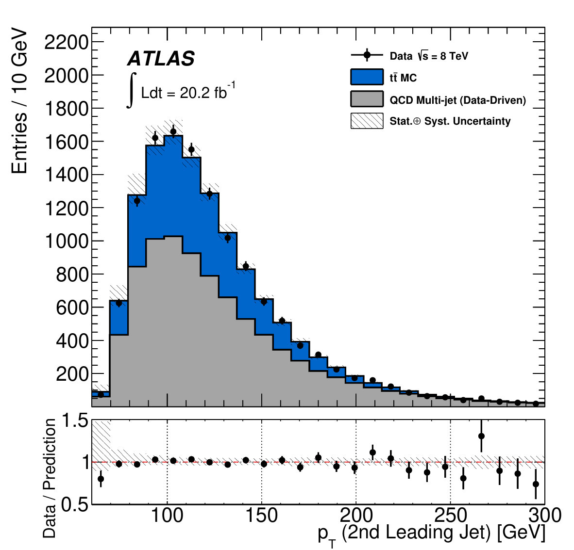 Figure 4
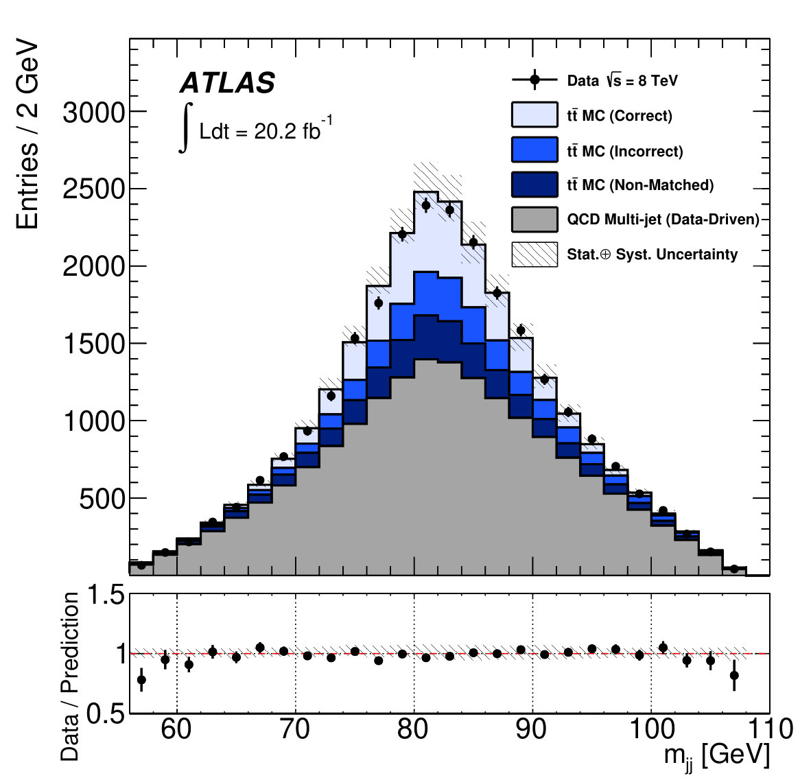 Figure 5
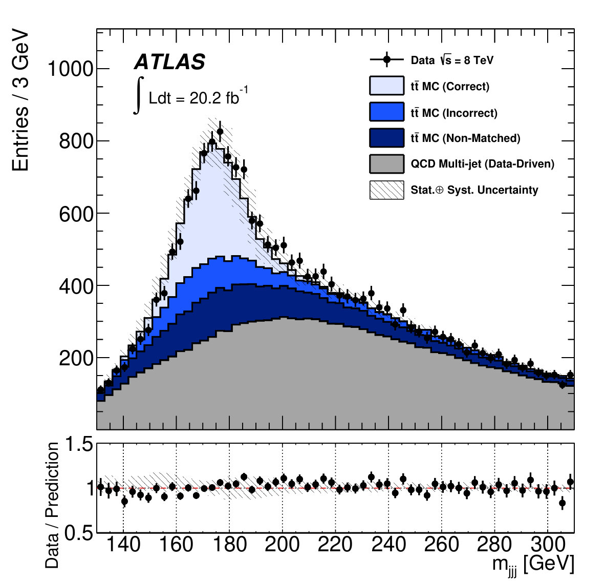 Figure 6
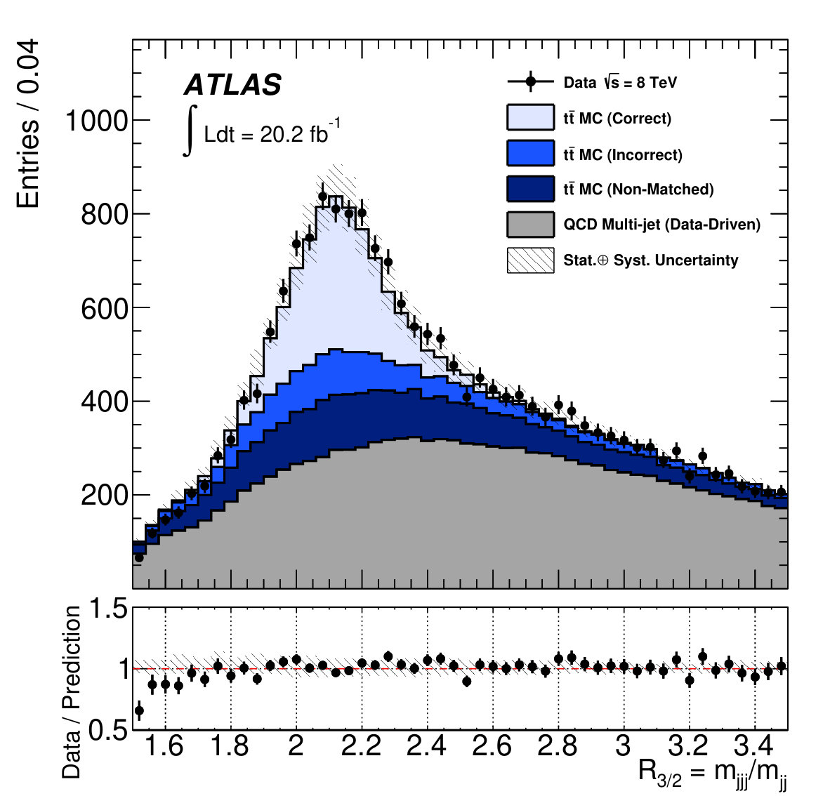 Figure 7
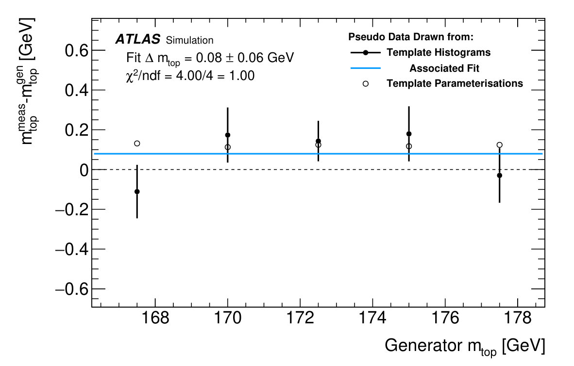 Figure 8
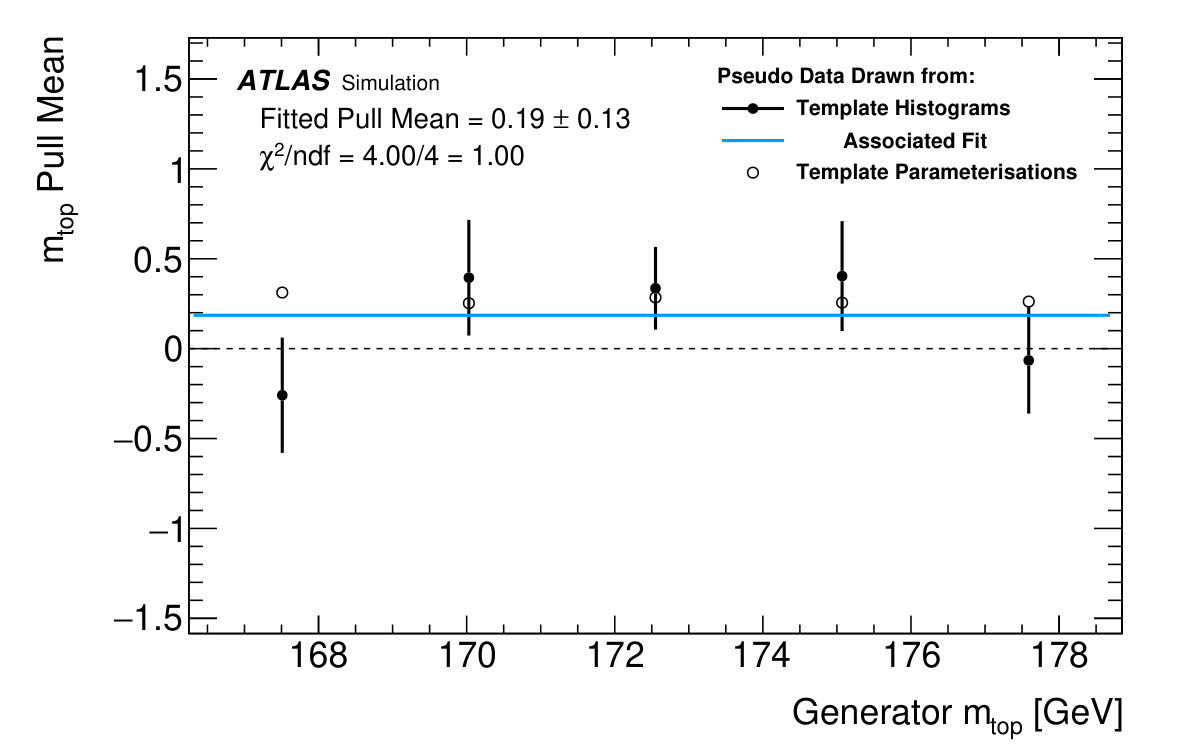 Figure 9
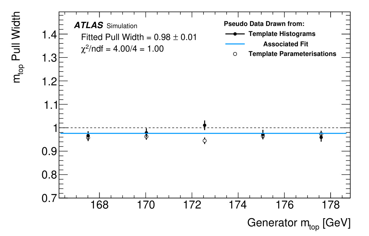 Figure 10
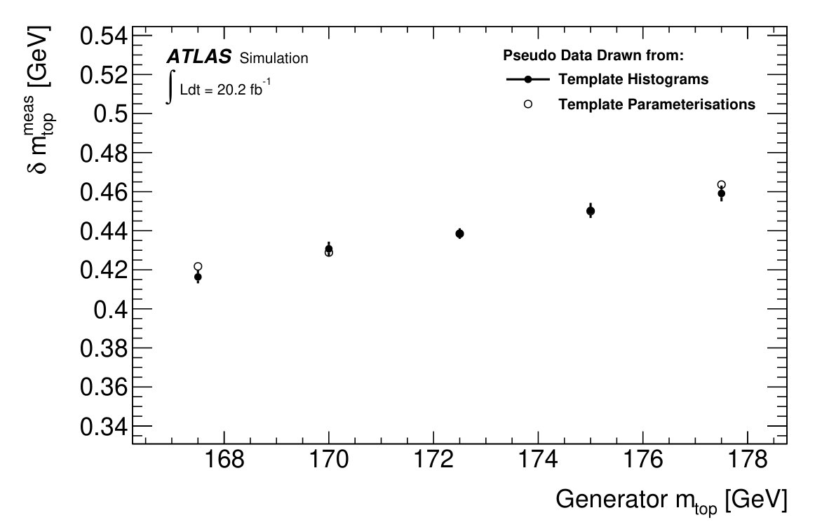 Figure 11
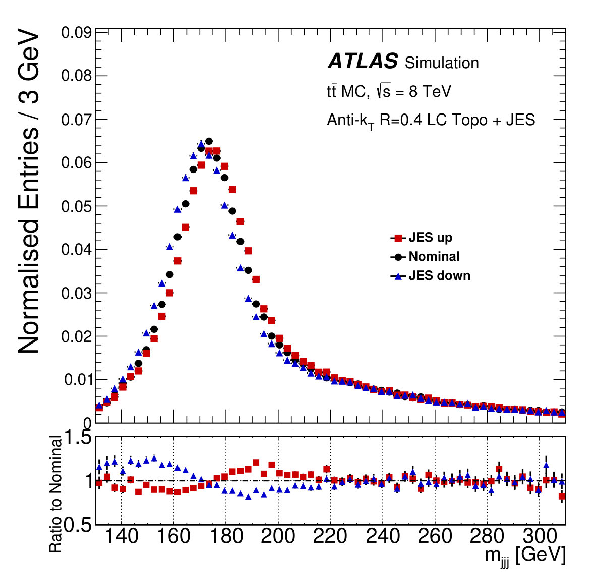 Figure 12
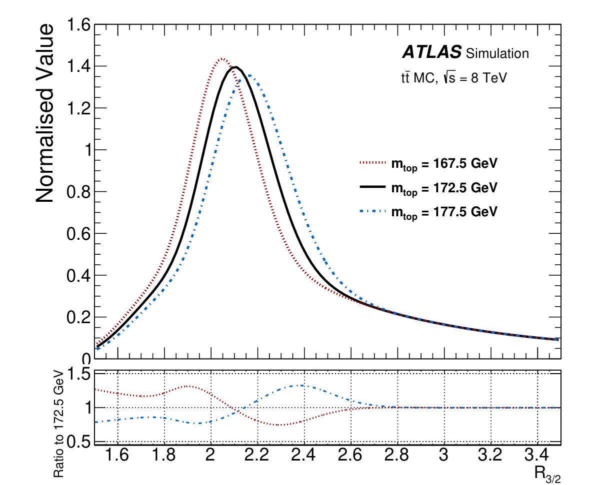 Figure 13
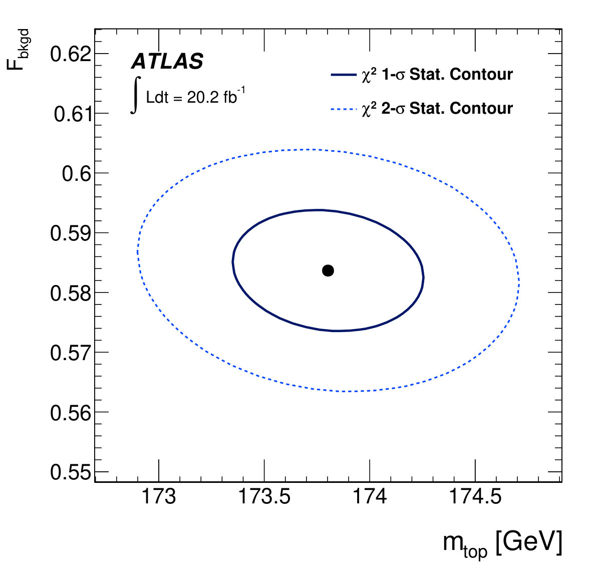 Figure 14
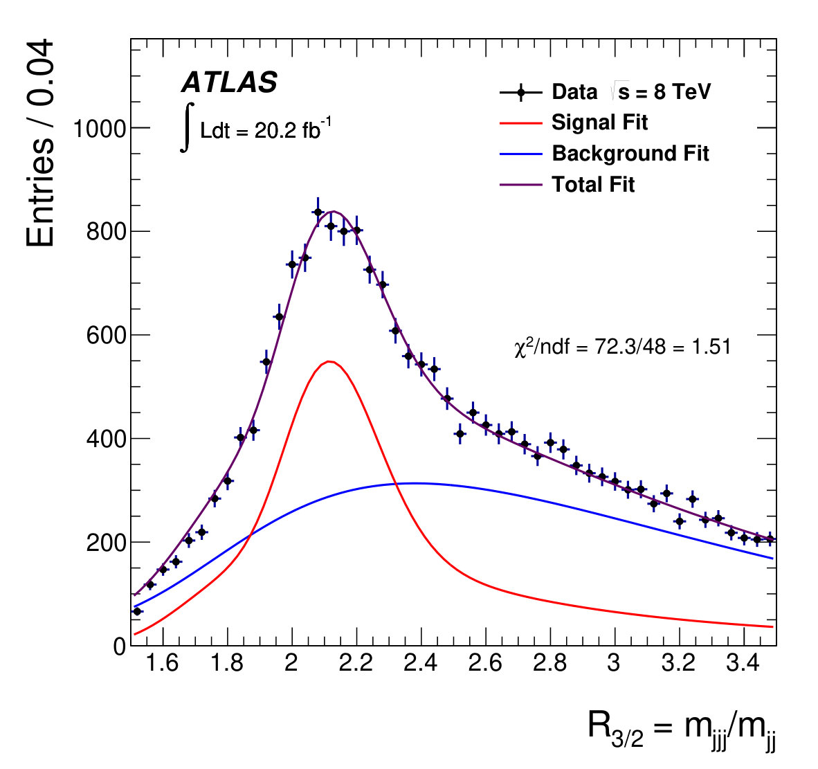 Figure 15
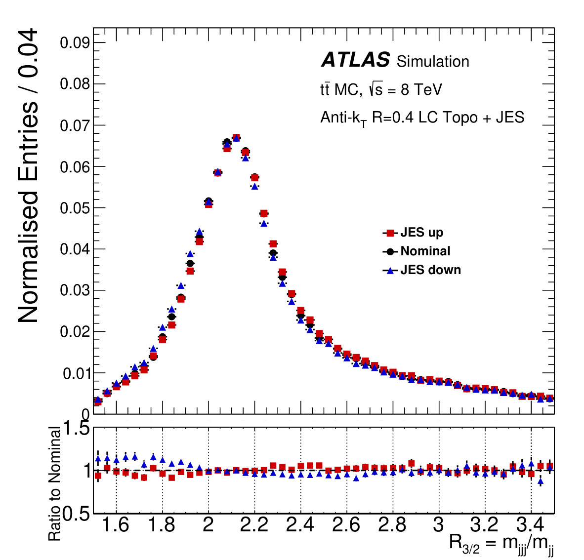 Figure 16
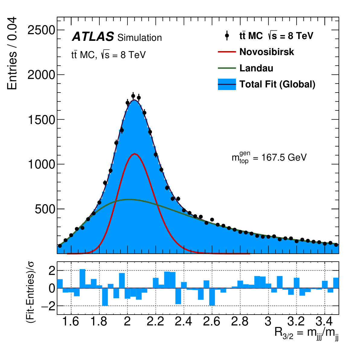 Figure 17
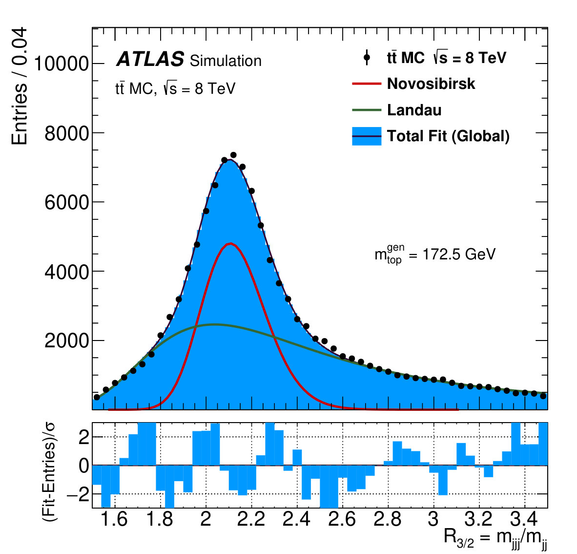 Figure 18
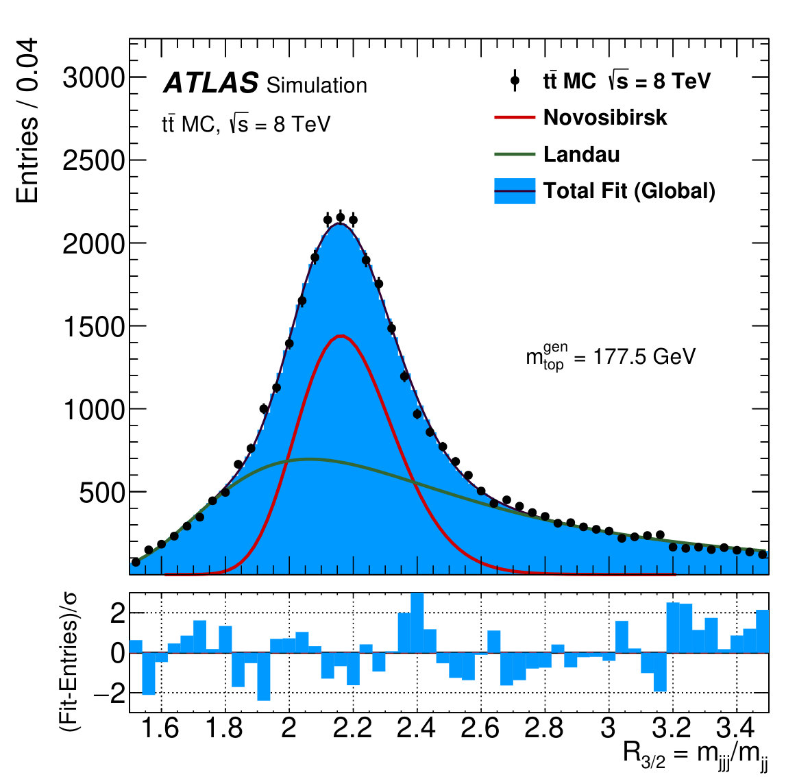 Figure 19
| Event yields (thousands) | ||||
|---|---|---|---|---|
| Cut | Data | all-hadronic (MC) | ||
| Initial | ||||
| & no isolated / | ||||
| Trigger: jets with & good jets | ||||
| No good jets () within | ||||
| good jets with | ||||
| () | ||||
| ABCD region and definition | Estimated signal fraction | ||||
| Region | MC/data [%] | ||||
| A | |||||
| B | |||||
| C | |||||
| D | |||||
| Source of uncertainty | [GeV] |
|---|---|
| Monte Carlo generator | |
| Hadronisation modelling | |
| Parton distribution functions | |
| Initial/final-state radiation | |
| Underlying event | |
| Colour reconnection | |
| Bias in template method | |
| Signal and bkgd parameterisation | |
| Non all-hadronic contribution | |
| ABCD method vs. ABCDEF method | |
| Trigger efficiency | |
| Lepton/ calibration | |
| Overall flavour-tagging | |
| Jet energy scale (JES) | |
| b-jet energy scale (bJES) | |
| Jet energy resolution | |
| Jet vertex fraction | |
| Total systematic uncertainty | |
| Total statistical uncertainty | |
| Total uncertainty |
| Region | A | B | C | D | E | F |
|---|---|---|---|---|---|---|
Peer Reviews
No public reviews on file for this paper yet. If you reviewed it on a platform where reviews are public (OpenReview, ICLR, NeurIPS, ICML), you can paste yours below so the community can read it here.
Videos
No videos yet. Explain this paper in a talk, walkthrough, or lecture? Add one.
\AtlasTitle
Top-quark mass measurement in the all-hadronic decay channel at 8\text{,}\text{Te\kern-1.00006ptV}$$ with the ATLAS detector
\PreprintIdNumberCERN-EP-2016-264 \AtlasJournalJHEP \AtlasAbstractThe top-quark mass is measured in the all-hadronic top-antitop quark decay channel using proton–proton collisions at a centre-of-mass energy of with the ATLAS detector at the CERN Large Hadron Collider. The data set used in the analysis corresponds to an integrated luminosity of . The large multi-jet background is modelled using a data-driven method. The top-quark mass is obtained from template fits to the ratio of the three-jet to the dijet mass. The three-jet mass is obtained from the three jets assigned to the top quark decay. From these three jets the dijet mass is obtained using the two jets assigned to the boson decay. The top-quark mass is measured to be 173.72\pm 0.55\mbox{;(stat.)}\pm 1.01\mbox{;(syst.)}\,\textrm{GeV}.
1 Introduction
Of all known fundamental particles, the top quark has the largest mass. Its existence was predicted in 1973 by Kobayashi and Maskawa [1], and it was not observed directly until 1995, by the CDF and D0 experiments at the Tevatron [2, 3]. Since 2010, top quarks have also been observed at the Large Hadron Collider (LHC) [4] at CERN. Due to the higher centre-of-mass energy, top quark production at the LHC is an order of magnitude larger than at the Tevatron. The large data sets of top–antitop quark () pairs allow many precision studies and measurements of top quark properties. The Yukawa coupling of the top quark is predicted to be close to unity [5, 6], suggesting that it may play a special role in electroweak symmetry breaking. In the Standard Model (SM), the top quark dominantly contributes to the quantum corrections to the Higgs self coupling [7, 8]. Precise measurements of the top-quark mass () are therefore very important in probing the stability of the vacuum [9, 10], and contribute to searches for signs of physics beyond the SM.
Today the most precise individual measurement of is in the single-lepton decay channel of top–antitop quark pairs, where one top quark decays into a -quark, a charged lepton and a neutrino and the other top quark decays into a -quark and two ///-quarks, performed by the CMS Collaboration, yielding a value of m_{\textrm{top}}=172.35\pm 0.16\mbox{;(stat.)}\pm 0.48\mbox{;(syst.)}\,\textrm{GeV} [11]. The most precise measurement of in the dileptonic decay channel, where each of the top quarks decays into a -quark, a charged lepton and its neutrino, is from the ATLAS Collaboration, yielding a value of m_{\textrm{top}}=172.99\pm 0.41\mbox{;(stat.)}\pm 0.74\mbox{;(syst.)}\,\textrm{GeV} [12]. Further results are available in Refs. [13, 14, 15].
The top-quark mass measurement in the all-hadronic channel takes advantage of the largest branching ratio (46%) among the possible top quark decay channels [16]. The all-hadronic channel involves six jets at leading order, two originating from -quarks and four originating from the two boson hadronic decays. It is a challenging measurement because of the large multi-jet background arising from various quantum chromodynamics (QCD) processes, which can exceed the production by several orders of magnitude. However, all-hadronic events profit from having no neutrinos among the decay products, so that all four-momenta can be measured directly. The multi-jet background for the all-hadronic channel, while large, leads to different systematic uncertainties than in the case of the single- and dileptonic channels. Thus, all-hadronic analyses offer an opportunity to cross-check top-quark mass measurements performed in the other channels. The most recent measurements of in the all-hadronic channel were performed by the CMS Collaboration with 172.32 0.25 \mbox{;(stat.)}\pm 0.59\mbox{;(syst.)}\,\textrm{GeV} [11], and the ATLAS Collaboration with m_{\textrm{top}}=175.1\pm 1.4\mbox{;(stat.)}\pm 1.2\mbox{;(syst.)}\,\textrm{GeV} [17].
This paper presents a top-quark mass measurement in the all-hadronic channel using data collected by the ATLAS experiment in 2012. The measurement is obtained from template fits to the distribution of the ratio of three-jet to dijet masses (), similarly to a previous measurement at [17]. The three-jet mass is obtained from the three jets assigned to the top quark decay. From the selected three jets the dijet mass is obtained using the two jets assigned to the boson decay. The jet assignment is accomplished by using a fit to the system, so there are two values of measured in each event. The observable employed in this analysis achieves a partial cancellation of systematic effects common to the masses of the reconstructed top quark and associated boson, notably the significant uncertainty on the jet energy scale. Data-driven techniques are used to estimate the contribution from multi-jet background events. Data events are divided into several disjoint regions using two uncorrelated observables. The region containing the largest relative fraction of events is labeled the signal region. The background is estimated from the other regions, which determine the shape of the background distribution in the signal region.
The paper is organised as follows. After a brief description of the ATLAS detector in Section 2, the data and Monte Carlo (MC) samples used in the analysis are described in Section 3. The analysis event selection is further detailed in Section 4. Section 5 describes the method used to select the candidate four-momenta that comprise the reconstructed system. The estimation of the multi-jet background is detailed in Section 6. The method used to measure the top-quark mass and its uncertainties are reported in Sections 7, 8, and 9. The results of the measurement are presented in Section 10, and the analysis is summarised in Section 11.
2 ATLAS detector
The ATLAS detector [18] is a multi-purpose particle physics experiment with a forward-backward symmetric cylindrical geometry and near coverage in solid angle 111The coordinate system used to describe the ATLAS detector is briefly summarised here. The nominal interaction point is defined as the origin of the coordinate system, while the beam direction defines the –axis and the – plane is transverse to the beam direction. The positive –axis is defined as pointing from the interaction point to the centre of the LHC ring and the positive –axis is defined as pointing upwards. The azimuthal angle is measured around the beam axis, and the polar angle is the angle from the beam axis. The pseudorapidity is defined as . The transverse momentum , the transverse energy , and the missing transverse momentum () are defined in the – plane unless stated otherwise. The distance in the – angle space is defined as .. The inner tracking detector (ID) covers the pseudorapidity range , and consists of a silicon pixel detector, a silicon microstrip detector, and, for , a transition radiation tracker. The ID is surrounded by a thin superconducting solenoid providing a magnetic field. A high-granularity lead/liquid-argon (LAr) sampling electromagnetic calorimeter covers the region . A steel/scintillator-tile calorimeter provides hadronic coverage in the range . LAr technology is also used for the hadronic calorimeters in the endcap region and for electromagnetic and hadronic measurements in the forward region up to . The muon spectrometer surrounds the calorimeters. It consists of three large air-core superconducting toroid systems, precision tracking chambers providing accurate muon tracking for , and additional detectors for triggering in the region .
3 Data and Monte Carlo simulation
This analysis is performed using the proton–proton () collision data set at a centre-of-mass energy of collected with the ATLAS detector at the LHC. The data correspond to an integrated luminosity of . Samples of simulated MC events are used to optimise the analysis, to study the detector response and the efficiency to reconstruct events, to build signal template distributions used for fitting the top-quark mass, and to estimate systematic uncertainties. Most of the MC samples used in the analysis are based on a full simulation of the ATLAS detector [19] obtained using GEANT4 [20]. Some of the systematic uncertainties are studied using alternative samples processed through a faster ATLAS simulation (AFII) using parameterised showers in the calorimeters [21]. Additional simulated collisions generated with Pythia [22] are overlaid to model the effects of additional collisions in the same and nearby bunch crossings (pile-up). All simulated events are processed using the same reconstruction algorithms and analysis chain as used for the data.
The nominal simulation sample is generated using the next-to-leading-order (NLO) MC program POWHEG-BOX [23, 24, 25] with the NLO parton distribution function (PDF) set CT10 [26, 27], interfaced to Pythia 6.427 [28] with a set of tuned parameters called the Perugia 2012 tune [29] for parton shower, fragmentation and underlying-event modelling. For the construction of the signal templates, MC events are generated at five different assumed values of , between and , in steps of . The full simulation of the ATLAS detector sample at has the largest number of generated events, and is used as the nominal signal sample. The parameter [30], which regulates the high- radiation in POWHEG-BOX, is set to the same value as used in each of the generated POWHEG-BOX samples. All the simulated samples used to estimate systematic uncertainties are further described in Section 9.
All MC samples are normalised using the predicted top–antitop quark pair cross-section () at . For , the next-to-next-to-leading-order cross-section of pb is calculated using the program Top++2.0 [31], which includes re-summation of next-to-next-to-leading logarithmic soft gluon terms.
4 Event selection
Events in this analysis are selected by a trigger that requires at least five jets with . Only events with a well-reconstructed primary vertex formed by at least five tracks with are considered for the analysis. Events with isolated electrons (muons) with () and reconstructed in the central region of the detector within are rejected. Both lepton types are identified using the tight working points as specified in Refs. [32, 33]. Jets () are reconstructed using the anti- algorithm with radius parameter [34] employing topological clusters [35] in the calorimeter. These jets are calibrated to the hadronic energy scale as described in Refs. [36, 37, 38]. The four-vector of the highest-energy muon () from among those matched within to a reconstructed jet, is added to the reconstructed jet four-vector. This is done to compensate for the energy losses in the calorimeter arising from semimuonic quark decays. In simulation this correction slightly improves both the jet energy response and resolution across the full range of jet energies.
To ensure that the selected events are in the plateau region of the trigger efficiency curve where the trigger efficiency in data is greater than %, at least five of the reconstructed central jets (within ) are required to have . Any additional jet is required to have and . All selected jets in an event must be isolated; any pairing of two jets ( and ) reconstructed with the above criteria are required to not overlap within . Events with jets failing this isolation requirement are rejected.
Events containing neutrinos are removed by requiring . The in an event is computed as the sum of a number of different terms [39, 40]. Muons, electrons and jets are accounted for using the appropriate calibrations for each object. For each term considered, the missing transverse momentum is calculated as the negative sum of the calibrated reconstructed objects, projected onto the and directions.
For the final selection, events are kept if at least two of the six leading transverse momentum jets are identified as originating from a -quark. Such jets are said to be -tagged. A neural network trained on decay vertex properties [41] is used to identify these -tagged jets. Because of the large number of -quarks originating from the boson decays in this analysis (on average one -quark per event) a -tagger trained to reject //-jets but also a large fraction of -jets is used. Events with fewer than two -tagged jets are used for the background estimate described in Section 6. The chosen working point for the -tagging neural network has an identification efficiency of about % [42] for jets from -quarks, with a rejection factor of about for jets arising from //-quarks, and a factor of about for jets arising from -quarks.
In each event the two jets with leading -tag weights ( and ) are required to satisfy . The quantities and represent here the vectorial transverse momentum of a -jet: and . This cut is very powerful in rejecting combinatorial background events; most of these are true events where the incorrect jets are associated with the top quark. Finally, a cut is applied based on the azimuthal angle between -jets and their associated boson candidate: the average of the two angular separations for each event is required to satisfy . Here the , and the are the vectorial transverse momentum of a -jet and a boson: and , identified by means of the three-jet combination that best fits the event hypothesis described in Section 5. This cut rejects a large fraction of events from the multi-jet and combinatorial backgrounds, as well as events from non-all-hadronic decays. Events failing this final selection cut are, however retained for the purpose of modelling the multi-jet background, as detailed in Section 6.
Table 1 summarises the yields obtained after each of the individual selection cuts. The cut listed in Table 1 is described in Section 5. The number of -tagged jets () and are the two observables used for the data-driven multi-jet background estimation, further detailed in Section 6.
5 reconstruction
In each event the final state is reconstructed using all the jets from the all-hadronic decay chain: . To determine the top-quark mass in each event, a minimum- approach is adopted, with the defined as:
[TABLE]
Here, two of the reconstructed jets are associated with the bottom-type quarks produced directly from the top quark and antitop quark decays ( and ), the other four jets are assumed to be ///-quark jets from the boson hadronic decay (, where ), and . This method considers all possible permutations of the six or more reconstructed jets in each event. The permutation resulting in the lowest value is kept. A low value indicates a permutation of jets consistent with the hypothesis. No explicit -tagging information is used in Eq. (1).
In each combination the reconstructed masses of the two hadronically decaying bosons ( and ) in data are compared to the mean of the mass distribution of correctly reconstructed bosons in simulated signal MC events (). The correct reconstruction of the top quarks and the bosons in a simulated event is achieved by matching parton-level particles to the event’s jets. The widths ( and ) used in the denominators of Eq. (1) are obtained from fits to a single Gaussian function to the mass distributions of the correctly reconstructed top quarks and bosons: \sigma_{\Delta m_{bjj}}=21.60\pm 0.16\mbox{;(stat.)}\,{\textrm{GeV}} and \sigma_{m_{W}^{\textrm{MC}}}=7.89\pm 0.05\mbox{;(stat.)}\,\textrm{GeV}. The mean value used in Eq. (1) is determined to be 81.18\pm 0.04\mbox{;(stat.)}\,\textrm{GeV}. To reduce the multi-jet background in the analysis and to eliminate events where the top quarks and the bosons in an event are not reconstructed correctly, a minimum is required.
6 Multi-jet background estimation
The available MC generators for multi-jet production include only leading-order theory calculations for final states with up to six partons. Therefore, the dominant multi-jet background in this analysis is determined directly from the data. Two largely uncorrelated variables are used to divide the data events into four different regions, such that the background is determined in the control regions and extrapolated to the signal region. The two chosen observables are the in an event, and the variable, both described in Section 4. These have a correlation measured in data of . The value of in each event is determined from the leading six jets ordered by .
The four regions, labelled ABCD, are identified by defining two bins in the number of -tagged jets, , , and two ranges of the variable, , , as detailed in Table 2. The distributions are studied for each of the defined regions. Region D represents the signal region (SR), and contains the largest fraction of events (%). Regions A, B, and C are the control regions (CR), and are dominated by multi-jet background events. Table 2 summarises the expected fractions of signal events in each of the four regions. Each signal fraction is estimated by comparing the total predicted number of signal events from simulation to the number of observed data events in each region.
To obtain an unbiased estimate of the number of background events in each considered CR, the signal contamination is removed using simulated events with . The method validation and the template closure described in Section 8 show that the dependence of this signal subtraction is significantly smaller than other uncertainties on the method, and is ignored. The estimated background in a given bin of for SR D () is given by:
[TABLE]
The background in a given bin of the spectrum of CR B () is estimated after subtraction of the signal contamination and after scaling by the ratio of the number events in control regions C () and A (), also after signal removal. The signal contamination present in CR C comes from improperly reconstructed events which form a smoothly varying distribution in . This signal contribution in CR C is not relevant in the analysis, as this region only affects the normalisation of the distribution obtained for the multi-jet background, which is not used in the fit for described in Section 7.
Figure 1 shows the distributions of the masses of the boson () and top quark () after applying the event selection, the approach defined in Eq. (1), and using the data-driven multi-jet background method. In the figure, the reconstruction using MC events is said to be correct for one (or both) top quark(s) if each of the three jets () selected by the reconstruction algorithm matches to each of the three quarks () within a , modulo the interchange of the two jets assigned to the hadronically decaying boson. If at least one of the jets selected by the algorithm is not one of the three jets matched to the quarks, the top quark reconstruction is classified as incorrect. Finally, events where at least one quark is not matched uniquely to a reconstructed jet are classified as non-matched. The distribution obtained after using the data-driven multi-jet background estimation methods to determine the shape and normalisation is shown in Figure 2. In general, good agreement between data and prediction is observed in all the distributions.
7 Top-quark mass determination
To extract a measurement of the top-quark mass, a template method with a binned minimum- approach is employed. For each event, two values are obtained, one for each top-quark mass measurement. To properly correct for the correlation between the two values in each event, the statistical uncertainty of returned from the final fit described later in this section is scaled up by a factor , where is the correlation factor as obtained from data. Signal and background templates binned in are created using the simulated events described in Section 3, and the data-driven background distribution.
The top quark contribution is parameterised by a probability distribution function (pdf) which is the sum of a Novosibirsk function [43] and a Landau function [44]. These describe, respectively, the signal and the combinatorial background. As a first step, the distributions from the five simulation samples with differing are fitted separately to determine the six parameters for each template mass. The MC simulation shows that each of these parameters depends linearly on the input . In the next step, the parameters are fitted to obtain the offsets and slopes of the linear dependencies. These values are then used as inputs to a combined, simultaneous fit to all five distributions. In total parameters are derived by the combined fit to determine the pdf. Figure 3 shows the distributions obtained using the MC samples based on the full simulation of the ATLAS detector and generated at three top-quark mass points: , , and . Results from the combined, simultaneous fit to all five distributions are superimposed. Shown are the functions describing the signal and combinatorial background, respectively, and their sum. The Novosibirsk mean and width parameters offer the strongest sensitivity to . Template distributions obtained simultaneously for three separate input values of (, , and ), highlighting the shape to , are shown in Figure 4.
The multi-jet background template distribution obtained from the output of the data-driven method described in Section 6 can be parameterised in a similar fashion. In this case the sum of a Gaussian function and a Landau function was found to be a suitable choice for the functional form. The background pdf requires five parameters.
As a final step in the parameterisation, in order to take properly into account the uncertainties and the correlations between the various signal and background shape parameters, a more generalised version of the function is used. The final fit, which uses matrix algebra to include non-diagonal covariance matrices, has the form:
[TABLE]
Here and are the two parameters which are left to float. The shape of the fitted multi-jet background parameterisation is assumed to be independent of while the normalisation, controlled by a background fraction parameter, , is obtained by fitting the data distribution. The is defined within the fit range of the distribution: . The term in Eq.(3) corresponds to the number of entries in bin in the data distribution, whereas corresponds to the estimated total number of signal and background entries. The term is the diagonal data covariance matrix with , which accounts for the statistical uncertainty in each bin . Similarly, and are non-diagonal covariance matrices which account for the signal and background shape parameterisation uncertainties and their correlations. In the distribution which has a total number of data entries , and a given bin width , the number of estimated entries in bin , , is given by:
[TABLE]
where and are the probability density functions for the signal and background, respectively.
8 Method validation and template closure
To validate the method employed to extract from the data distribution and to check for any potential bias, a series of pseudo experiments are performed. For each of the five simulated samples a total of pseudo experiments generating a distribution of the variable are produced 222This value of is also used when performing pseudo experiments to estimate the systematic uncertainties.. Two scenarios are investigated: in the first one, events are drawn randomly from template distributions; in the second scenario, events are drawn directly from the signal and background shapes. In each scenario the nominal values of all signal and background shape parameters are used, and only two parameter values, and , are returned from the minimisation procedure. For all five top-quark mass MC samples, the same multi-jet background distribution is used for drawing pseudo events.
The value of obtained from each pseudo experiment () is used to fill a distribution of the difference between these values and the values used for event generation. This distribution is then fitted with a Gaussian function, giving estimators for the Gaussian mean and width parameters, each with their respective uncertainties. The uncertainty in the fitted mean is corrected for the oversampling that is induced by drawing from template distributions produced using a finite number of MC events [45]. The fitted mean , referred to as the “difference mean”, is shown in Figure 5. Fitting the difference mean for the five top-quark mass samples with a linear function gives an -independent bias of . The treatment of this small bias is further discussed in Section 9.2.
Pull distributions are constructed in an analogous way, where the pull in each pseudo experiment is defined as:
[TABLE]
where is the statistical uncertainty of the parameter obtained from the fit of the pseudo experiment. The correction that takes into account the correlation between two values in each event, described in Section 7, is not applied here, as the values of drawn for pseudo experiments are uncorrelated. The pull distribution for an unbiased measurement has a mean of zero and a standard deviation of unity. A fitted pull mean value of and a fitted pull width of are obtained, which shows that the uncertainty determination is unbiased.
9 Systematic uncertainties
This section outlines the various sources of systematic uncertainty in which are summarised in Table 3. All sources are treated as uncorrelated. Individual contributions are symmetrised and the total uncertainty is taken as the sum in quadrature of all contributions.
The majority of the systematic uncertainties are assessed by varying the MC sample to reflect the uncertainty from each of these sources. Pseudo experiments are constructed from the varied sample, which are then passed through the analysis chain; the change in the result relative to that obtained from the nominal MC sample is evaluated. Exceptions to this are described in the following subsections. To facilitate a combination with other results, each systematic uncertainty is assigned a statistical uncertainty, taking into account the statistical correlation of the considered samples. Following Ref. [46], the systematic uncertainties listed in Table 3 are calculated independently of the statistical uncertainties of the values.
In what follows, each source of systematic uncertainty is briefly described. These are broken down into three categories. The first category, theory and modelling uncertainties, is associated with the simulation of the signal events. The second set of uncertainties is related to the analysis method. These involve uncertaintie due to the way that the analysis was performed, including the choice of a template method, the background modelling, and the final extraction procedure. Finally a third category, calibration- and detector-related uncertainties involves uncertainties coming from the standard calibrations of physics objects.
9.1 Theory and modelling uncertainties
Monte Carlo generator:
In order to assess the impact on the measurement due to the choice of MC generator, the results of pseudo experiments using two different AFII simulated samples are compared: one sample produced using POWHEG-BOX as the MC generator and a second sample using MC@NLO [47]. Both samples use Herwig 6.520.2 [48] with the AUET2 tune to model the parton shower, hadronisation and underlying event, in contrast with the nominal signal MC where Pythia 6.427 is used. The absolute difference of between the resulting average parameter returned from the fits is accounted for as the uncertainty.
Hadronisation modelling:
To quantify the expected change in the measured value due to a different choice of hadronisation model, pseudo experiments are performed for two independent MC samples both employing POWHEG-BOX AFII simulation to generate the all-hadronic events but differing in their choice of hadronisation model. In the first case, Pythia 6.427 [28] is used to model the parton shower, hadronisation and underlying event with the Perugia 2012 tunes [29], while in the second case, Herwig 6.520.2 with the AUET2 tune [48] is used. The absolute difference of between the average values obtained in the two cases is accounted for as the systematic uncertainty.
Parton distribution functions:
A variety of PDF sets are investigated in order to assess the impact of the choice of CTEQ10 [26, 27], the default PDF set used in the nominal measurement. There are a total of distinct sets for the CTEQ PDFs. In addition there are distinct NNPDF23 [49] PDF sets and distinct MSTW2008 [50, 51] PDF sets to consider, giving a total of distinct sets to compare. Simulated POWHEG-BOX+Herwig [23, 24, 25, 48] events are used for the comparison. The individual PDF uncertainty contributions are evaluated according to set-dependent procedures as described in Ref. [52] for CT10 [27, 26], for MSTW [49], and for NNPDF [50, 51]. To determine the final systematic uncertainty, the quantity is calculated for each of the three sets, where is the measured value from the central reference sample of the corresponding PDF set. Half of the difference between the largest and the smallest of these values is quoted as the symmetrised final uncertainty, and is .
Initial-state and final-state radiation:
Varying the amount of initial- and final-state radiation (ISR and FSR) can have an impact on the number of reconstructed jets, which in turn can affect the overall measurement of the top-quark mass. In order to quantify the sensitivity of the measurement to ISR/FSR, two alternative POWHEG-BOX plus Pythia 6.427 [28] AFII samples are used. The first sample has the parameter [30] set to 2, the factorisation and renormalisation scale 333The default POWHEG-BOX factorisation and renormalisation scales are set to decreased by a factor of and uses the Perugia 2012 radHi tune [29], giving more parton shower radiation. The second sample has the Perugia 2012 radLo tune, and the factorisation and renormalisation scale increased by a factor of , giving less parton shower radiation. Half of the absolute difference between the measured values from the pseudo experiments is quoted as the corresponding systematic uncertainty and is .
Underlying event:
Additional semi-hard multiple parton interactions (MPI) present in the hard-scattering can change the kinematics of the underlying event. The number of such additional semi-hard MPI is a Perugia 2012 tunable parameter [29] in the Pythia 6.427 generator [28]. Simulated AFII events were produced with an increased number of semi-hard MPI (Perugia 2012 mpiHi) in order to assess the potential impact on the final measurement. The absolute difference between the results of these pseudo experiments and the one using the nominal simulated AFII sample is quoted as the systematic uncertainty and is .
Colour reconnection:
When simulating AFII signal events using Pythia 6.427 [28] for the parton shower and hadronisation modelling, there is a tunable parameter associated with the colour reconnection strength due to the colour flow along parton lines in the strong-interaction hard-scattering process. An alternative AFII sample uses the Pythia Perugia 2012 loCR tune [29], which corresponds to reduced colour reconnection strength. The absolute difference of between the results of these pseudo experiments and the average value obtained using the nominal Pythia 6.427 events is quoted as the systematic uncertainty.
9.2 Method-dependent uncertainties
Bias in template method:
Based on the results of the closure tests, a small bias is observed in the extracted top-quark mass. By drawing pseudo events from the parameterisations an offset of about in the mass difference () is present (see Figure 5). The offset does not exhibit a dependence on the generator’s value. For this reason the parameter value returned from a fit to the average bias from pseudo experiments across is subtracted from the final value as measured in data. The final value of quoted in this analysis includes this subtraction. The uncertainty in this fitted offset is then quoted as the systematic uncertainty of associated with the template method’s non-closure.
Signal and background parameterisation:
To extract as described in Section 7, the uncertainties in the shape parameters of the observable for the signal contributions are included in the covariance matrices which enter into the minimisation used to extract (see Eq. (3)). Omitting these contributions would yield a simplified definition of the variable:
[TABLE]
which can be recognised as the standard definition of the variable for a least-squares fit assuming only a diagonal covariance matrix. The fit to the data distribution is repeated using this simplified definition of the variable. This results in a slightly modified returned value of the parameter and a smaller statistical uncertainty. The difference in quadrature of between the final statistical uncertainty returned from the original minimisation and this modified value is quoted as the uncertainty in the signal and background parameterisation.
Inclusion of non-all-hadronic background:
A number of event selection requirements, such as the lepton veto and the requirement that , result in a large suppression of background contributions arising from non-all-hadronic events. The estimated fractional contribution from such events in the final signal region is below %, and is not considered in the nominal case. Pseudo experiments are performed by drawing events from the nominal signal distribution but from a modified background, now consisting of QCD events and events with at least one leptonic boson decay. The absolute difference of between the average value obtained in this way and that from the nominal case is quoted as a systematic uncertainty.
Variation in the number of control regions:
A variation of the background estimation procedure is considered in which six distinct regions, rather than four, are defined to estimate the multi-jet background. This is done by allowing three different values of : [math], , or . Events can then be separated into the six differing regions as in the nominal analysis. As in the nominal case the number of -tagged jets in an event considers only the leading six jets, ordered by . The values of the second ABCD variable, , are unchanged from the nominal case. One reason for considering this alternative is that the inclusion of a larger number of control regions could potentially provide sensitivity to different physics processes. Additionally, the systematic uncertainty contribution arising from uncertainties in the -tagging scale factors could differ between these methods.
With a total of six regions shown in Table 4 the background estimation technique remains similar to that using four regions.
The final SR is labelled F. The new region D, together with region B, is now used to predict the shape of the multi-jet background in SR F, whereas CR A, C, and E set the multi-jet background normalisation [17]. Pseudo experiments are performed by drawing background events from the modified multi-jet distribution in the final signal region. The absolute difference of between this and the nominal case is quoted as the systematic uncertainty.
9.3 Calibration- and detector-related uncertainties
Trigger efficiency:
The trigger efficiency obtained using simulated signal events [23, 24, 25, 28, 29] is compared to an equivalent distribution obtained using data, which results in a small observed discrepancy. The data here are expected to consist primarily of multi-jet events. It is expected that some true kinematic differences give rise to the difference observed between the data and MC trigger efficiencies. In order to obtain a conservative uncertainty, it is assumed that the difference represents a mis-modelling of the data by the trigger simulation. The simulated events are assigned a -dependent trigger efficiency correction such that the corrected MC and data trigger efficiencies agree. Pseudo experiments are performed by drawing signal events from the modified distribution with the trigger SFs applied, and the absolute difference from the nominal case is quoted as a conservative uncertainty on due to the trigger efficiency.
Pile-up reweighting scale:
The distribution of the average number of interactions per bunch crossing, denoted by , is known to differ between data and simulation. Simulated events are reweighted so that matches the value observed in data. In order to assess the impact on the final result, pseudo experiments are performed in which the reweighting scale is shifted up and down according to its uncertainty, and the fit procedure is repeated. A negligible maximum change of in is found as the symmetrised up/down uncertainty.
Lepton and soft-term calibrations:
Uncertainties in the calibration scales and in the resolutions of the lepton () four-vector objects [53, 33, 54] can potentially lead to small differences in the event selection or the jet–quark assignment in the top reconstruction algorithm. Similarly, small uncertainties in can be expected due to the uncertainties in the scale and resolution of the soft term [39, 40]. The soft term is varied according to these uncertainties and pseudo experiments are performed with the modified MC events. In the case of the muon-related uncertainties, Gaussian smearing is performed to assess the impact on the final result. The maximum absolute deviation from the reference value is taken as the uncertainty in each case, and these are added in quadrature to obtain a single value of for all lepton- and -related scale and resolution uncertainties.
Flavour-tagging efficiencies:
In the validation of the flavour-tagging algorithms, the differences between tagging efficiencies and mis-tag rates evaluated in data and simulation are removed by applying scale factor (SF) weights to the simulated events. The uncertainties in the flavour-tagging SFs are calculated separately for the -tagging SFs, the -tagging SFs, and the overall mis-tag SFs [42]. The uncertainties in the flavour-tagging SFs are split into various components. The full covariance matrix between the various bins of jet transverse momentum is built and decomposed into eigenvectors. Each eigenvector corresponds to an independent source of uncertainty, each with an upward and a downward fluctuation, and the resulting total systematic uncertainty is .
Jet energy scale:
The different contributions to the total JES uncertainty are estimated individually as described in Ref. [36]. For each component the resulting differences from the up and down variations, corresponding to one-standard-deviation relative to the nominal JES, are quoted separately. The total uncertainty for each contribution is taken as half of the absolute difference between the up and down variation. In case both the up and down variations result in a change in the parameter in the same direction, the largest absolute difference (either from the up or down variation) is taken as the symmetrised uncertainty. The total JES uncertainty is the sum in quadrature of all subcontributions, and is . This includes all but the -jet energy scale contribution, which is quoted separately and discussed below.
-jet energy scale:
The reconstructed top quark four-momenta are sensitive to the energy scale of jets initiated by -quarks, particularly as a result of choices in the fragmentation modelling. Based on the uncertainties associated with the -jet energy scale [55], a similar up/down variation procedure is performed using pseudo experiments and the quoted systematic uncertainty of is half the absolute difference between the two variations.
Jet energy resolution:
An eigenvector decomposition strategy similar to that followed for the JES and the flavour-tagging systematic uncertainties is used for the determination of jet energy resolution (JER) systematic uncertainties [56]. The final quoted JER systematic uncertainty is .
Jet reconstruction efficiency:
A small difference between the jet reconstruction efficiencies measured in data and simulation was observed [37], and as this difference can affect the final measured value, a set of pseudo experiments are performed in which jets from simulated events are removed at random. The frequency of this is chosen such that the modified jet reconstruction efficiency in simulation matches the value measured in data. The analysis is repeated with this change and no significant difference is observed.
10 Measurement of
After applying the method described in Section 7 the top-quark mass is measured to be:
[TABLE]
The statistical error quoted in Eq. (7) is corrected for the correlation between the two measurements of each event, as discussed in Section 7. The systematic uncertainty quoted above is the sum in quadrature of all the systematic uncertainties described in Section 9 and summarised in Table 3. Figure 6 shows the distribution (left plot) with the corresponding total fit as well as its decomposition into signal and the multi-jet background. The right plot in this figure shows the ellipses corresponding to - (solid line) and - (dashed line) variations in statistical uncertainty. This measurement agrees with the previous all-hadronic measurement performed by ATLAS in [17] data, with the measurements performed in the single-lepton and dileptonic decay channels [14, 15, 11, 12] and with the results of combining the Tevatron and LHC measurements [13].
11 Conclusion
From the analysis of 20.2\,\mbox{fb{}^{-1}} of data recorded with the ATLAS detector at the LHC at a centre-of-mass energy of , the top-quark mass has been measured in the all-hadronic decay channel of top–antitop quark pairs to be
[TABLE]
This measurement is obtained from template fits to the observable, which is chosen due to its reduced dependence on the jet energy scale uncertainty. The dominant remaining sources of systematic uncertainty, despite the usage of the observable, come from the jet energy scale, hadronisation modelling and the -jet energy scale. This measurement agrees with the previous Tevatron and LHC measurements, and with the results of Tevatron and LHC combinations. It is about % more precise than the previous measurement performed by ATLAS in the all-hadronic channel at .
Acknowledgements
We thank CERN for the very successful operation of the LHC, as well as the support staff from our institutions without whom ATLAS could not be operated efficiently.
We acknowledge the support of ANPCyT, Argentina; YerPhI, Armenia; ARC, Australia; BMWFW and FWF, Austria; ANAS, Azerbaijan; SSTC, Belarus; CNPq and FAPESP, Brazil; NSERC, NRC and CFI, Canada; CERN; CONICYT, Chile; CAS, MOST and NSFC, China; COLCIENCIAS, Colombia; MSMT CR, MPO CR and VSC CR, Czech Republic; DNRF and DNSRC, Denmark; IN2P3-CNRS, CEA-DSM/IRFU, France; GNSF, Georgia; BMBF, HGF, and MPG, Germany; GSRT, Greece; RGC, Hong Kong SAR, China; ISF, I-CORE and Benoziyo Center, Israel; INFN, Italy; MEXT and JSPS, Japan; CNRST, Morocco; FOM and NWO, Netherlands; RCN, Norway; MNiSW and NCN, Poland; FCT, Portugal; MNE/IFA, Romania; MES of Russia and NRC KI, Russian Federation; JINR; MESTD, Serbia; MSSR, Slovakia; ARRS and MIZŠ, Slovenia; DST/NRF, South Africa; MINECO, Spain; SRC and Wallenberg Foundation, Sweden; SERI, SNSF and Cantons of Bern and Geneva, Switzerland; MOST, Taiwan; TAEK, Turkey; STFC, United Kingdom; DOE and NSF, United States of America. In addition, individual groups and members have received support from BCKDF, the Canada Council, CANARIE, CRC, Compute Canada, FQRNT, and the Ontario Innovation Trust, Canada; EPLANET, ERC, ERDF, FP7, Horizon 2020 and Marie Skłodowska-Curie Actions, European Union; Investissements d’Avenir Labex and Idex, ANR, Région Auvergne and Fondation Partager le Savoir, France; DFG and AvH Foundation, Germany; Herakleitos, Thales and Aristeia programmes co-financed by EU-ESF and the Greek NSRF; BSF, GIF and Minerva, Israel; BRF, Norway; CERCA Programme Generalitat de Catalunya, Generalitat Valenciana, Spain; the Royal Society and Leverhulme Trust, United Kingdom.
The crucial computing support from all WLCG partners is acknowledged gratefully, in particular from CERN, the ATLAS Tier-1 facilities at TRIUMF (Canada), NDGF (Denmark, Norway, Sweden), CC-IN2P3 (France), KIT/GridKA (Germany), INFN-CNAF (Italy), NL-T1 (Netherlands), PIC (Spain), ASGC (Taiwan), RAL (UK) and BNL (USA), the Tier-2 facilities worldwide and large non-WLCG resource providers. Major contributors of computing resources are listed in Ref. [57].
The reference list from the paper itself. Each links out to its DOI / PubMed record.
- 1[1] Makoto Kobayashi and Toshihide Maskawa “CP Violation in the Renormalizable Theory of Weak Interaction” In Prog. Theor. Phys. 49 , 1973, pp. 652–657 DOI: 10.1143/PTP.49.652 · doi ↗
- 2[2] CDF Collaboration and F. Abe “Observation of top quark production in p ¯ p ¯ 𝑝 𝑝 \bar{p}p collisions” In Phys. Rev. Lett. 74 , 1995, pp. 2626–2631 DOI: 10.1103/Phys Rev Lett.74.2626 · doi ↗
- 3[3] D 0 Collaboration and S. Abachi “Observation of the top quark” In Phys. Rev. Lett. 74 , 1995, pp. 2632–2637 DOI: 10.1103/Phys Rev Lett.74.2632 · doi ↗
- 4[4] Lyndon Evans and Philip Bryant “LHC Machine” In JINST 3 , 2008, pp. S 08001 DOI: 10.1088/1748-0221/3/08/S 08001 · doi ↗
- 5[5] T. D. Lee “A Theory of Spontaneous T 𝑇 T Violation” In Phys. Rev. D 8 American Physical Society, 1973, pp. 1226–1239 DOI: 10.1103/Phys Rev D.8.1226 · doi ↗
- 6[6] Steven Weinberg “Unitarity Constraints on CP Nonconservation in Higgs Exchange” In Phys. Rev. D 42 , 1990, pp. 860–866 DOI: 10.1103/Phys Rev D.42.860 · doi ↗
- 7[7] W. Hollik “Electroweak theory” In 5th Hellenic School and Workshops on Elementary Particle Physics (CORFU 1995) Corfu, Greece, September 3-24 , 1995 ar Xiv: hep-ph/9602380 [hep-ph]
- 8[8] Michael E. Peskin “On the Trail of the Higgs Boson” In Annalen Phys. 528.1-2 , 2016, pp. 20–34 DOI: 10.1002/andp.201500225 · doi ↗