This paper develops a refined semiclassical second microlocal calculus for linear coisotropic submanifolds in the torus, enabling detailed analysis of wavefront sets and propagation of coisotropic regularity for eigenfunctions and quasimodes.
Contribution
It introduces a new second microlocal calculus for coisotropic submanifolds in the torus and establishes propagation theorems for coisotropic wavefronts, extending classical microlocal analysis.
Findings
01
Proves propagation theorems analogous to Hörmander's for coisotropic wavefronts.
02
Shows invariance of coisotropic wavefront under Hamiltonian flow expansions.
03
Provides tools for analyzing regularity and singularities of eigenfunctions and quasimodes.
Abstract
We develop a semiclassical second microlocal calculus of pseudodifferential operators associated to linear coisotropic submanifolds C⊂T∗Tn, where Tn=Rn/Zn. First microlocalization is localization in phase space T∗Tn; second microlocalization is finer localization near a submanifold of T∗Tn. Our second microlocal operators test distributions on Tn (e.g., Laplace eigenfunctions) for a coisotropic wavefront set, a second microlocal measure of absence of \emph{coisotropic regularity}. This wavefront set tells us where, in the coisotropic, and in what directions, approaching the coisotropic, a distribution lacks coisotropic regularity. We prove propagation theorems for coisotropic wavefront that are analogous to H\"{o}rmander's theorem for pseudodifferential operators of real…
No public reviews on file for this paper yet. If you reviewed it on a platform where reviews are public (OpenReview, ICLR, NeurIPS, ICML), you can paste yours below so the community can read it here.
Videos
No videos yet. Explain this paper in a talk, walkthrough, or lecture? Add one.
Taxonomy
TopicsAdvanced Mathematical Physics Problems · Spectral Theory in Mathematical Physics · Geometric Analysis and Curvature Flows
Full text
Semiclassical second microlocalization at linear coisotropic submanifolds in the torus
Rohan Kadakia
Abstract.
We develop a semiclassical second microlocal calculus of pseudodifferential operators associated to linear coisotropic submanifolds C⊂T∗Tn, where Tn=Rn/Zn. First microlocalization is localization in phase space T∗Tn; second microlocalization is finer localization near a submanifold of T∗Tn.
Our second microlocal operators test distributions on Tn (e.g., Laplace eigenfunctions) for a coisotropic wavefront set, a second microlocal measure of absence of coisotropic regularity. This wavefront set tells us where, in the coisotropic, and in what directions, approaching the coisotropic, a distribution lacks coisotropic regularity.
We prove propagation theorems for coisotropic wavefront that are analogous to Hörmander’s theorem for pseudodifferential operators of real principal type. Furthermore, we study the propagation of coisotropic regularity for quasimodes of semiclassical pseudodifferential operators. We Taylor expand the relevant Hamiltonian vector field, partially in the characteristic variables, at the spherical normal bundle of the coisotropic. Provided the principal symbol is real valued and depends only on the fiber variables in the cotangent bundle, and the subprincipal symbol vanishes, we show that coisotropic wavefront is invariant under the first two terms of this expansion.
A submanifold C of the symplectic manifold (T∗X,ω)
is said to be coisotropic if (TC)ω⊂TC; in words, C is coisotropic if the symplectic orthocomplement to its tangent bundle is a subbundle of the tangent bundle itself.
Most distributions encountered while studying PDE are not O(h∞). (O(h∞) is the semiclassical analogue of C∞ smoothness.) Some of these distributions, however, possess a different type of regularity—they are coisotropic distributions, associated to a coisotropic submanifold C. We say that u=uh∈L2(X) (uniformly as h↓0) is coisotropic if for all k and all semiclassical pseudodifferential operators (PsDO) A1,…,Ak∈Ψh(X) with σpr(Aj)↾C≡0, we have
[TABLE]
Here, σpr(A) is the semiclassical principal symbol of A. We may, by restricting the microsupports of the characteristic operators Aj, refine coisotropic regularity to be local on C.
The central idea in this paper is that of second microlocalization at a linear coisotropic submanifold C of T∗Tn, where Tn=Rn/Zn. To (first) microlocalize is to localize in symplectic phase space, i.e., to simultaneously localize in position and momentum (up to the uncertainty principle). Second microlocalization is more refined localization near a submanifold. The first step is to blow upC, which technically means that we replace C with its spherical normal bundle SN(C) (cf. [23], [25, Chapter 5]).
Next, for our second microlocal pseudodifferential calculus Ψ2,h(C), the collection of symbols consists of functions that are smooth on the blown up space. In particular, this includes functions singular on the original (i.e., blown down) space with conormal singularities, resolved in the blowup. Thus, Ψ2,h(C) contains the ordinary pseudodifferential calculus Ψh(Tn) as a subalgebra111Technically, as we see later, only PsDO with compactly supported symbols may be regarded as elements of Ψ2,h(C)..
Associated to the calculus Ψ2,h(C) is a wavefront set 2WF in SN(C), whose absence (together with absence of standard semiclassical wavefront WFh in T∗Tn\C) is equivalent to u being a coisotropic distribution. A helpful analogy is that presence of second wavefront set in SN(C) is to failure of coisotropic regularity in C as presence of homogeneous wavefront in the cotangent bundle is to singular support in the base. 2WF tells us where, in the coisotropic, and in what directions, approaching the coisotropic, a distribution lacks coisotropic regularity; for instance, see Example 4.6.4.
Whether in the homogeneous or semiclassical setting, several instances of second microlocalization exist in the literature: A. Vasy and J. Wunsch in the special case of Lagrangian submanifolds [29]; N. Anantharaman, C. Fermanian, and F. Macià in [1, 2, 3] to study defect measures; and J-M. Bony’s [4] second microlocalization at conic Lagrangians. To study resonances, J. Sjöstrand and M. Zworski [28] construct a second microlocal calculus for hypersurfaces. Additional sources are [5, 8, 10, 17, 18, 20, 21].
Every coisotropic submanifold is endowed with a characteristic foliation. The leaves of the characteristic foliation of C are the integral curves of the Hamiltonian vector fields of its defining functions. All of our results pertain specifically to linear coisotropic submanifolds. As coordinates on (T∗Tn,ω), we take (x,ξ), where ω=dξ∧dx. Then, a d-codimensional linear coisotropic is of the form C=Tn×{v1⋅ξ=…=vd⋅ξ=0} for vj∈Rn.
1.1. Propagation of coisotropic second wavefront set
First, we show by commutator methods the analogue of Hörmander’s real principal type theorem [14]:
Theorem 1.1.1**.**
Let P∈Ψ2,h(C) and suppose that P has real valued second principal symbol 2σpr(P). Assume also that the distribution u satisfies Pu=f. Then 2WF(u)\2WF(f) is invariant under Hamiltonian flow at SN(C).
For the next result, we consider an ordinary semiclassical PsDO P∈Ψh(Tn), regarded as an element of the second microlocal calculus. Further, we require that the principal symbol of P depends only on the fiber variables ξ, and that its subprincipal symbol vanishes. We calculate the Hamiltonian vector field H for 2σpr(P). Then we Taylor expand H at SN(C): if SN(C)={ρ=0}, then H=H1+ρH2+O(ρ2).
Theorem 1.1.2**.**
Assume P∈Ψh(Tn) has real principal symbol depending only on the fiber variables in the cotangent bundle, that its subprincipal symbol vanishes, and that Pu=OL2(Tn)(h∞). Then 2WF(u)∩SN(C) is invariant under both H1 and H2.
This crucially hinges on P being an ordinary semiclassical PsDO, so having a total symbol that is smooth even on the blown down space T∗Tn.
The author is supported in part by NSF RTG grant 1045119. He would like to thank Jared Wunsch for introducing him to the problems addressed in this paper, and for helpful discussions throughout. The author is grateful also to Dean Baskin and Alejandro Uribe. Much of this work was carried out at Northwestern University.
2. Preliminaries
Let (M,ω) be a 2n-dimensional symplectic manifold. We will be interested in the case M=T∗Tn. For a submanifold C⊂M, consider the symplectic orthocomplement(TC)ω of the tangent bundle TC, defined as the union of its fibers:
[TABLE]
Definition 2.0.1** (Coisotropic submanifold).**
C is said to be a coisotropic submanifold of M if (TC)ω is a subbundle of TC; that is, C is coisotropic if (TpC)ω is a subspace of TpC for each p∈C.
In particular, this means that dim(C)≥n. If dim(C)=n, then C is a Lagrangian submanifold.
2.1. Coisotropic regularity
For m,k∈R, let Ψhm,k(Tn)=h−kΨhm(Tn) be the space of semiclassical pseudodifferential operators of differential order m. For treatments of the semiclassical pseudodifferential calculus, see [9, 22, 33]. Let
[TABLE]
The symbol class Sm is due to J.J. Kohn and L. Nirenberg [19]. Then Ψhm,k(Tn) consists locally of quantizations of symbols in h−kC∞([0,1)h;Sm(T∗Tn)).
Let A∈Ψhm,k(Tn). We will generally not be interested in the differential order of A, which corresponds to the behavior of its total symbol at infinity in the fibers of the cotangent bundle. Thus, we define the subalgebra Ψhk(Tn)⊂Ψh−∞,k(Tn) consisting locally of quantizations of h−kCc∞(T∗Tn×[0,1)h) (i.e., the total symbols are compactly supported in the fibers) plus quantizations of h∞C∞([0,1);S−∞(T∗Tn)) (symbols residual in both semiclassical and differential filtrations). This is the same subalgebra considered in the motivating paper [29].
2.1.1. Characteristic operators
Let C be any coisotropic submanifold of T∗Tn. Consider
[TABLE]
We call this the module of characteristic operators associated to C. An application of Taylor’s theorem proves that MC is finitely generated. It is closed under commutators, as well. To see this, take A,B∈MC.
Recall that [A,B] has principal symbol ih{σ0(A),σ0(B)}. Since {σ0(A),σ0(B)}=LHσ0(A)(σ0(B)), Hσ0(A) is tangent to C, and σ0(B) is constant on C, then {σ0(A),σ0(B)}↾C=0.
As an example, if C={ξ1=…=ξd=0}, the module MC is generated by the differential operators hDxj, 1≤j≤d.
Remark 2.1.1**.**
If we write uh∈L2(Tn), we mean that uh lies in L2 uniformly in h as h↓0. We will suppress h dependence of families of distributions. Likewise, we will write P instead of Ph when referring to the family of operators Ph.
2.1.2. Definition of coisotropic regularity
Definition 2.1.2** (Coisotropic regularity).**
Let C be a coisotropic submanifold of T∗Tn. A distribution u∈L2(Tn) is said to exhibit coisotropic regularity with respect to C at the point (x,ξ)∈C if (x,ξ) has a neighborhood U⊂T∗Tn such that for all Pj∈MC microsupported in U, we have
[TABLE]
(for all k).
Suppose that u has coisotropic regularity everywhere on C. Then we call u a coisotropic distribution or simply say that u is coisotropic. Or, if condition (2.1.2) holds only for k0≤k for some k, then u has coisotropic regularity of order k at (x,ξ).
Remark 2.1.3**.**
(1) We may write the defining condition for coisotropic regularity of u∈L2(Tn) equivalently as
[TABLE]
Note that since each Pj is a semiclassical PsDO of order 0 in h, it is a bounded operator on L2, so necessarily P1…Pku∈L2(Tn). By contrast, h−1Pj∈Ψh1(Tn) will generally not be L2 bounded.
(2) We are certainly not the first to define a notion of regularity by means of iterated application of characteristic operators. The original iterated regularity characterization, of conic Lagrangian distributions, is given by L. Hörmander and R. Melrose [15, Section 25.1].
Example 2.1.4**.**
To determine whether some u∈L2(T3) is (globally) coisotropic with respect to C={ξ1=ξ2=0,ξ3∈R}, amounts to checking for L2-Sobolev regularity in the directionsx1 and x2. For instance, eix3/h is a coisotropic distribution with respect to C, but eix1/h is nowhere coisotropic at C.
2.1.3. Coisotropic regularity, extended
For s∈R, we may consider the set of distributions that are coisotropic of order k∈Z≥0 relative to hsL2(Tn):
[TABLE]
However, because MC is (locally) finitely generated, let {B1,…,BJ} be a generating set. To check whether u lies in I(s)k(C), it suffices to check h−∣β∣−sBβu∈L2(Tn), where Bβ=B1β1⋯BJβJ and 0≤∣β∣≤k.
We may extend the definition of I(s)k(C) to k∈R by interpolation (to k∈R≥0) and duality (to negative k). For each s, I(s)∞(C) is a space of semiclassical coisotropic distributions.
2.2. Real blowup of submanifolds
For a thorough treatment of this topic, see R. Melrose’s notes in [23] and [25, Chapter 5]. If M is a manifold without boundary and Y is any submanifold of M, then Y blown up in M is [M;Y]=M\Y∪SN(Y). Here, SN(Y) is the spherical (unit) normal bundle of Y. [M;Y] is a manifold with boundary, and the boundary of [M;Y] is SN(Y).
Next, suppose M is a manifold with boundary and Y is a submanifold lying in the boundary of M. Then the blowup of M along Y is [M;Y]=M\Y∪SN+(Y), where SN+(Y) is the inward pointing part of the spherical normal bundle to Y in M. SN+(Y) is the front face of the blowup, and the side face is ∂M\Y. There is a smooth blowdown mapβ:[M;Y]⟶M projecting the front face to Y; β is a diffeomorphism away from the front face. Thus, crucially, there are more smooth functions on the blown up space than on the original manifold. In our case, M=T∗Tn×[0,1)h (which has boundary T∗Tn×{h=0}) and Y=C×{h=0}.
2.3. Linear coisotropics
We study linear coisotropics in T∗Tn, defined as follows:
Definition 2.3.1**.**
A d-codimensional linear coisotropic submanifoldC⊂T∗Tn has the form
[TABLE]
where {v1,…,vd}⊂Rn is linearly independent over R.
A simple linear coisotropic is {ξ1=…=ξd=0}. In fact, locally every coisotropic is of this form [15, Theorem 21.2.4].
2.4. Second microlocal symbols
The domain of our total symbols is the manifold with corners Stot:=[T∗Tn×[0,1)h;C×{h=0}]. The corner occurs at the intersection of the front face SN+(C×{h=0}) and the side face. Second principal symbols (defined in Section 4) live on Spr:=[T∗Tn;C], which is identifiable with the side face of Stot.
Example 2.4.1**.**
In Figure 1, we see the total symbol space for the coisotropic C=T2×{ξ1∈R,ξ2=0}, with base variables omitted. Notice that the front face is a half cylinder. Since we are not interested in negative values of h, only (unit) normal vectors pointing into the interior of T∗T2×[0,1)h are considered.
In Spr, we replace C⊂T∗Tn with its full spherical normal bundle. Let ρff and ρsf denote boundary defining functions for the front and side faces of Stot, respectively.
Definition 2.4.2** (Total symbols).**
For m,l∈R, let
[TABLE]
We define
[TABLE]
Remark 2.4.3**.**
Here we clarify that we are considering two different spherical normal bundles. First, there is the inward-pointing spherical normal bundle SN+(C×{h=0}), which is the front boundary face of Stot. Second, there is the full spherical normal bundle to C⊂T∗Tn, namely SN(C). The principal symbol space Spr is a manifold with boundary, with ∂Spr=SN(C). Finally, SN(C) is identifiable with the corner of Stot.
Let dˉξ:=(2πh)−ndξ. Let hOpl, hOpW, and hOpr represent semiclassical left, Weyl, and right quantization, respectively: For a∈Sm,l(Stot),
[TABLE]
Also, if a∈C∞(Tn;Sm,l(Stot)), then
[TABLE]
χ is any cutoff function supported in a neighborhood of the diagonal, and χ≡1 in a smaller neighborhood of the diagonal. The purpose of χ is to make sense of the difference (x−y) appearing in the phase. A stationary phase argument shows that the choice of a particular χ does not matter, up to O(h∞).
Our calculus will be denoted Ψ2,h(C). The calculus will consist of, say, left quantizations of elements of Sm,l(Stot) (m,l∈R), as well as residual operators to be introduced in Section 3.
3. Composition and Invariance
Let C=Tn×{v1⋅ξ=…=vd⋅ξ=0}, with vi∈Rn linearly independent.
3.1. Residual operators
We next define the “residual” elements which, along with quantizations of symbols, comprise the second microlocal calculus Ψ2,h(C). Residual operators play the same role as smoothing operators in the C∞ pseudodifferential calculus.
Let Bj=vj⋅hDx, where Dx=(Dx1⋯Dxn)t. Then B1,…,Bd∈Ψh0(Tn) generate the module MC of operators characteristic on C, and let Bβ:=B1β1⋯Bdβd be a monomial formed from these generators. Also, let Bj=vj⋅Dx and Bβ=B1β1⋯Bdβd.
Definition 3.1.1** (Residual operator).**
For l∈R, the bounded linear operator R is in the residual space ℜl if:
Condition 3.1.2**.**
R is involutizing: for uh∈L2(Tn) and multi-indices β,γ, R satisfies
[TABLE]
(Since we are composing B on the right of R, if this condition is fulfilled, then the adjoint operator R∗ is also involutizing.)
Let ℜ:=⋃l∈Rℜl. Then:
Definition 3.1.3**.**
The second microlocal calculus associated to C is
[TABLE]
We will show that Ψ2,h(C) is closed under composition. The key result is a reduction theorem, Theorem 3.2.1. The calculus is also closed under asymptotic summation: if Aj∈Ψ2,hm−j,l(C), then there exists A∈Ψ2,hm,l(C) for which
[TABLE]
for all N.
3.2. Reduction and Composition
Theorem 3.2.1** (Right reduction).**
Let a(x,y,ξ;h)∈C∞(Tn;Sm,l(Stot)). Then there exists b∈Sm,l(Stot) such that Ih(a)=hOpr(b)+R, and the remainder R belongs to ℜl.
Before we prove this theorem, we state and prove a result concerning boundedness.
Proposition 3.2.2** (L2 boundedness).**
Let s∈Cc∞(Tn×Stot). Then Ih(s)∈Ψ2,h0,0(C) is bounded on L2(Tn).
This parallels the standard result that h-pseudodifferential operators in Ψh0(Tn) (here, [math] is the order in the h-filtration, not the differential order) are L2 bounded. The following is an essential ingredient of our proof of L2 boundedness.
Lemma 3.2.3** (Calderón–Vaillancourt theorem).**
Let a(x,y,ξ;h)∈Cc∞(Tn×Tn×Rn×[0,1)). Suppose that for all multi-indices α,β, there exists a constant Cαβ>0 (independent of h) such that
[TABLE]
Then
[TABLE]
is bounded, as an operator on L2(Tn). (Note that this is a non-semiclassical quantization.)
Let s∈Cc∞(Tn×Stot) and change variables η=ξ/h. Then the estimate in (3.2.1) becomes
[TABLE]
Using a partition of unity, we may decompose s into pieces supported on Tn times the lift to Stot of {vj⋅ξ=0}×[0,1)h⊂T∗Tn×[0,1)h for j=1,…,d. By symmetry, it is enough to study the part of s supported on Tn times the lift of {v1⋅ξ=0}×[0,1).
We may extend the linearly independent set {v1,…,vd} to a basis
[TABLE]
for Rn. Locally, in a neighborhood of the corner of Stot, we employ the coordinates x, y, H=h/(v1⋅ξ), ζ=v1⋅ξ,
[TABLE]
and W=(wd+1⋅ξ,…,wn⋅ξ).
We lift h∣β∣∂x,yα∂ξβ to the coordinates just introduced, then show that s satisfies the estimate in (3.2.2) under application of the lifted vector field. In particular, we will lift h∂ξi for 1≤i≤n. We have
[TABLE]
where wi=(wd+1i,…,wni). Let vi=(v2i,…,vdi). We calculate that
[TABLE]
Therefore,
[TABLE]
For 1≤i≤n, ∣h∂ξis∣ is thus bounded (independently of h), because s∈Cc∞(Tn×Stot) is compactly supported in the variables ζ, H, W, and Ξ.
Therefore, since (3.2.2) is satisfied, we may apply the Calderón–Vaillancourt theorem to conclude that Ih(s):L2(Tn)→L2(Tn).
∎
Let Vb represent the set of vector fields on Stot tangent to both front and side faces. Notice that V∈Vb. Now we prove Theorem 3.2.1.
Proof.
We use the same coordinates as in the previous proof, and let ρsf=H=h/(v1⋅ξ), ρff=ζ=v1⋅ξ.
Let a(x,y,ξ;h)∈C∞(Tn;Sm,l(Stot)). Taylor’s formula yields the asymptotic sum
[TABLE]
We see from (3.2.3) that for all 1≤j≤n, application of h∂ξj to a second microlocal total symbol improves its decay at the side face. Therefore, for any multi-index α,
[TABLE]
so there exists b∈H−mζ−lCc∞(Stot) for which
[TABLE]
Fix any N. Then
[TABLE]
and
[TABLE]
We have
[TABLE]
Let RN:=Ih(aN)−hOpr(bN)∈Ψ2,hm−N,l(C). We will show that the operator Ih(aN) is residual as defined above, ‘up to order N’ (see below). The proof for hOpr(bN) is the same, except bN has one fewer component.
Proof of Condition 3.1.2: We are interested in h−∣β∣BβIh(aN). By the Leibniz rule, this equals
[TABLE]
Recall that H−1=(v1⋅ξ)/h is the reciprocal of the boundary defining function for the side face. Hence, as long as ∣β∣≤−m+N+l, the net contribution is a positive power of ρsf.
Ih(aN)Bγ is handled similarly. Note that the amplitude aN is smooth in x and y, so application of B does not change the symbol class to which aN belongs. By Proposition 3.2.2, we conclude that Ih(aN) is involutizing for ∣β∣+m−l≤N.
Similarly, Ih(a−aN),hOpr(b−bN)∈Ψ2,hm−N,l(C) are finitely residual in this sense. Then, since
[TABLE]
we may conclude that Ih(a)−hOpr(b) is residual.
∎
We can likewise prove a left reduction or Weyl reduction. The point is that we can convert one quantization map into any other, at the (low) cost of one of these residual operators.
Corollary 3.2.4** (Composition Law).**
If a∈Sm,l(Stot), b∈Sm′,l′(Stot), then hOpl(a)∘hOpl(b)=hOpl(c)+R for c∈Sm+m′,l+l′(Stot) and R∈ℜl+l′.
Proof.
By Theorem 3.2.1, it is sufficient to consider hOpl(a)∘hOpr(b). We have
[TABLE]
For this integral, we use the stationary phase theorem [33, Theorem 3.17], and we concisely write the amplitude as s(w,η;h). By this theorem, for all N
[TABLE]
Note that (∂wjχ)(y,y)=0 and likewise for higher order derivatives of χ, since these are supported off the diagonal. Thus, writing out the first few terms of the sum,
[TABLE]
We know (∂wjχ)(x,y), and all higher derivatives evaluated at w=y, is supported off-diagonal. So the contributions of these terms are residual (i.e., the kernel of a second microlocal operator is a coisotropic distribution, associated to C×C, away from the diagonal). Note that for all j, (h∂ηjb)(y,η;h) is a second microlocal symbol, due to (3.2.3).
By Theorem 3.2.1, we can then write (3.2.4) as the left quantization of some c∈Sm+m′,l+l′(Stot), modulo a residual remainder.
∎
From now on, we will not explicitly write χ. By definition, the adjoint of a residual operator in ℜl is again an element of ℜl. In addition, it is routine to prove:
Proposition 3.2.5**.**
Let A=hOpl(a) for a∈Sm,l(Stot). Then A∗∈Ψ2,hm,l(C).
Moreover, it is reassuring that quantizations of elements of S−∞,l(Stot), l∈R, are residual.
Proposition 3.2.6**.**
Suppose C is a linear coisotropic. If A=hOpr(a) for a∈S−∞,l(Stot), then A∈ℜl.
Proof.
Locally in Stot, we may take v1⋅ξ as defining function for the front face and h/(v1⋅ξ) for side face defining function.
We show that A satisfies Condition 3.1.2. Recall that Bj=vj⋅Dx and Bβ=B1β1∘⋯∘Bdβd; also, let V=(v1⋅ξ,…,vd⋅ξ). We have
[TABLE]
No matter how large β is, ρsf−∣β∣a∈S0,l(Stot). Therefore, BβA maps L2(Tn) to h−lL2(Tn).
∎
Finally, we show:
Proposition 3.2.7**.**
The residual algebra is an ideal in Ψ2,h(C).
Proof.
Let a∈Sm,l(Stot) and A=hOpr(a). Let R∈ℜl′. We show that AR∈ℜl+l′. Taking adjoints then implies RA∈ℜl+l′.
Let Θxj=vj⋅Dx and Θxβ=Θx1β1⋯Θxdβd. Then, for u∈L2(Tn),
[TABLE]
The bracketed term lies in L2, since R is involutizing. And hlhOpr(Θyμa)∈Ψ2,hm−l,0(C) so, if m≤l, it is L2 bounded. Instead, if m>l, choose p≥m−l. As before, locally we may take ρsf=h/v1⋅ξ as side face defining function. Then for μ+ν=β,
[TABLE]
[TABLE]
This time, the amplitude belongs to Sm−l−p,0(Stot), so by Proposition 3.2.2 the operator is L2 bounded. Thus, AR satisfies Condition 3.1.2.
Meanwhile, it is easily seen that for R1∈ℜl, R2∈ℜl′, we have R1R2∈ℜl+l′.
∎
4. Microsupport, parametrices & second wavefront
4.1. Second microsupport
Let Stot and Spr be symbol spaces associated to any linear coisotropic C. Recall that Spr may be identified with the side face of Stot.
Definition 4.1.1**.**
For a∈Sm,l(Stot), define the essential support of a by:
[TABLE]
If A=hOpr(a) for a∈Sm,l(Stot), then the second microsupport2WFl′(A) of A is given by 2WFl′(A):=esssuppl(a). If A∈ℜl, define 2WFl′(A)=∅.
Second microsupport obeys the usual laws of microsupports:
Proposition 4.1.2**.**
Let A,B∈Ψ2,hm,l(C), D∈Ψ2,hm′,l′(C). Then 2WF′ satisfies
[TABLE]
4.2. Principal symbols of second microlocal operators
Let A∈Ψ2,hm,l(C). Suppose A=hOpr(a)+R for some a∈Sm,l(Stot) and residual operator R∈ℜl.
Definition 4.2.1**.**
The principal symbol of A is
[TABLE]
But the pair (a,R) is not unique. Suppose we also have a′∈Sm,l(Stot), R′∈ℜl such that A=hOpr(a′)+R′. Then
[TABLE]
Thus, while a priorihOpr(a−a′)∈Ψ2,hm,l(C), in fact hOpr(a−a′)∈ℜl. This principal symbol will be well defined if it is independent of the choice of right reduction. This amounts to showing that the difference a−a′, which a priori belongs to Sm,l(Stot) for whatever value of m∈R, in fact decays at the side face of Stot. We claim the stronger result that a−a′∈S−∞,l(Stot).
Lemma 4.2.2**.**
For b∈Sm,l(Stot), suppose that hOpr(b)∈ℜl. Then b∈S−∞,l(Stot).
Proof.
Let C={v1⋅ξ=…=vd⋅ξ=0} as usual. We use the same coordinates in Stot as in the proof of Proposition 3.2.2: ρff=v1⋅ξ, Ξ, and W. (Note that ρsf=h/(v1⋅ξ), as we must have ρff×ρsf=h.)
Expand b in powers of ρsf, near the corner {ρsf=ρff=0}:
[TABLE]
the coefficients bj can be taken to be smooth functions on the side face.
Next, suppose b=O(ρsf∞). Then there must exist a coefficient bj0 which is nontrivial at the corner. By continuity of bj0, we have bj0 nontrivial in a neighborhood {ρff<ϵ} (also localized in x, Ξ, and W); i.e., there exists a point (x0,ρff0>0,Ξ0,W0) at which bj0 is nonzero. So ρsfj0bj0=O(h∞) at (x0,ρsf=0,ρff0,Ξ0,W0). Hence hOpr(b) cannot lie in ℜl, since ℜl reduces to O(h∞) along the side face. (More generally, Ψ2,h(C) is really just Ψh(Tn) microlocally away from the coisotropic.)
∎
Set 2charm,l(A):={ρffl−m2σm,l(A)=0}. That is, the second characteristic set is the zero set of a smooth function on the principal symbol space. We abuse notation by omitting the indices and writing 2charm,l simply as 2char. The complementary notion is
[TABLE]
Note that these definitions are independent of choice of front face defining function. Next, we state some essential properties of the principal symbol map.
Lemma 4.2.3**.**
[TABLE]
is a short exact sequence. Furthermore, the principal symbol map is a homomorphism: if A∈Ψ2,hm,l(C), B∈Ψ2,hm′,l′(C), then 2σm+m′,l+l′(AB)=2σm,l(A)2σm′,l′(B).
The proof is straightforward, so we omit it.
Remark 4.2.4**.**
If A∈Ψ2,hm,l(C), B∈Ψ2,hm′,l′(C), then
[TABLE]
where the Poisson bracket is computed with respect to the symplectic form on Spr lifted from the symplectic form on T∗Tn. See also Remark 5.1.2.
Remark 4.2.5**.**
For each m∈R, Ψhm(Tn) can be identified with a subset of Ψ2,hm,m(C). Locally, each element A∈Ψhm(Tn) is a quantization of a symbol a∈h−mCc∞(T∗Tn×[0,1)h) (or a is residual in both semiclassical and differential filtrations). If βtot:Stot→T∗Tn×[0,1) is the (smooth) blowdown map, then the pullback βtot∗a quantizes to the corresponding element A∈Ψ2,hm,m(C). Likewise, we may identify the principal symbol of A∈Ψhm(Tn) with the second principal symbol of A∈Ψ2,hm,m(C).
4.3. Global Parametrices
Lemma 4.3.1**.**
Suppose that A∈Ψ2,hm,l(C) is globally elliptic (i.e., 2σm,l(A) vanishes nowhere). Then there exist B,C∈Ψ2,h−m,−l(C) for which AB−Id∈ℜ0, CA−Id∈ℜ0; and B and C differ by an element of ℜ−l.
Proof.
An iterative construction similar to the proof of [32, Theorem 3.4].
∎
4.4. Microlocal Parametrices
Let C={v1⋅ξ=…=vd⋅ξ=0} for vi∈Rn. Let A∈Ψ2,hm,l(C). We partition the principal symbol space Spr, and restrict our focus to the lift L1 of {v1⋅ξ=0}⊂T∗Tn (we have likewise partitioned Stot). Extend {v1,…,vd} to a basis
[TABLE]
for Rn. Near the corner SN(C)=∂Spr, valid coordinates are x, ζ=v1⋅ξ,
[TABLE]
h=0 on the entirety of Spr.
Lemma 4.4.1**.**
Take a point p=(x,ζ,Ξ,W)∈2ell(A)∩L1. Then there exists B∈Ψ2,h−m,−l(C) such that
[TABLE]
Proof.
Similar to the construction of microlocal parametrix presented in Lemma 4.3 of [24], but adapted to the second microlocal setting.
∎
A neat consequence of microlocal parametrices is the following elliptic regularity result:
Corollary 4.4.2**.**
Suppose P∈Ψ2,hm,l(C) is elliptic on the microsupport of A∈Ψ2,hm′,l′(C):
[TABLE]
Then there exists a second microlocal operator A0∈Ψ2,h−m+m′,−l+l′(C) such that A=A0P+ℜl′.
4.5. Mapping Properties
As usual, let C={v1⋅ξ=…=vd⋅ξ=0}. Next, for k,s∈R, we give an alternative characterization of I(s)k(C) (these spaces of distributions were defined in (2.1.3)):
Lemma 4.5.1**.**
[TABLE]
Proof.
For simplicity, we may as well assume s=0. We prove the lemma directly for k∈Z≥0; interpolation and duality then give the full result.
Assume u∈I(0)k(C). For x∈Tn, (x,ξ)∈C if and only if (v1⋅ξ)2+…+(vd⋅ξ)2=0. So
[TABLE]
belongs in MC. Hence, h−1B∈Ψh1(Tn) and (h−1B)ku∈L2(Tn). At the same time, we take ρff=∣(v1⋅ξ,…,vd⋅ξ)∣ as front face defining function. The symbol of (h−1B)k is h−k∣(v1⋅ξ,…,vd⋅ξ)∣2k, which lifts to ρsf−kρffk, so (h−1B)k∈Ψ2,hk,−k(C)⊂Ψ2,hk,0(C)222Really we should first ‘cut off’ B so its symbol is compactly supported in the fibers. Then only can it be regarded as a second microlocal operator. Similarly for the Bj in the subsequent paragraph. (since k≥0). Then A=(I+h−1B)k
is an elliptic operator satisfying Au∈L2(Tn).
Conversely, consider the generators B1,…,Bd, Bj=vj⋅hDx, of MC. Suppose there exists elliptic A∈Ψ2,hk,0(C) such that Au∈L2(Tn). Let 0≤∣β∣≤k. Then there exists a parametrix A′∈Ψ2,h−k,0(C) such that
[TABLE]
Note that h−∣β∣Bβ∈Ψ2,h∣β∣,0(C) (for each 1≤j≤d, vj⋅ξ is a locally valid defining function for the front face). By Proposition 3.2.7, h−∣β∣BβR∈ℜ0, so the latter summand in the RHS above lies in I(0)∞(C)⊂L2(Tn). Since ∣β∣≤k, h−∣β∣BβA′∈Ψ2,h0,0(C), so Proposition 3.2.2 implies that h−∣β∣BβA′(Au)∈L2(Tn).
∎
Lemma 4.5.2** (Mapping Property).**
For m∈R and l≥0, P∈Ψ2,hm,l(C) satisfies
[TABLE]
for each k,s∈R. In particular, if R∈ℜl, then
[TABLE]
Since I(0)0(C)=L2(Tn), this property generalizes Proposition 3.2.2. Define
[TABLE]
Fh is the semiclassical Fourier transform. We see that the I(s)k-norm is a partial Sobolev norm with respect to the characteristic derivatives.
Proof.
Take u∈I(s)k(C). By Lemma 4.5.1, there is an elliptic operator A∈Ψ2,hk,0(C) for which Au∈hsL2(Tn). Choose P∈Ψ2,hm,l(C). We want to prove there exists elliptic A∈Ψ2,hk−m,0(C) satisfying APu∈hs−lL2(Tn). Let A be any elliptic element of Ψ2,hk−m,0(C). At the same time, since A is elliptic, there exists B∈Ψ2,h−k,0(C) such that BA−Id=R∈ℜ0. Therefore,
[TABLE]
APR∈ℜl (by Proposition 3.2.7) and APB∈Ψ2,h0,l(C). Since u∈hsL2(Tn), certainly we have (APR)u∈hs−lL2(Tn). And since l≥0, hlAPB∈Ψ2,h−l,0(C) maps hsL2 into itself, by Proposition 3.2.2.
∎
4.6. Second Wavefront Set
Definition 4.6.1**.**
For any m,l∈R, the m,l-graded second wavefront set of a distribution u∈I(l)−∞(C) is
[TABLE]
Let u∈I(l)−∞(C). We will later use the containment property
[TABLE]
Also, put 2WF∞,l(u)=⋃m∈R2WFm,l(u), so that
[TABLE]
Notice that 2WF∞,l(u)=∅ if and only if u∈I(l)∞(C), i.e., u is a coisotropic distribution.
We see that 2WFm,l(u)⊂Spr. Away from the coisotropic, this new wavefront is the same as standard semiclassical wavefront set:
[TABLE]
Just as the semiclassical pseudodifferential calculus Ψh does not spread singularities as measured by WFh, we have:
Lemma 4.6.2**.**
Let A∈Ψ2,hm′,l′(C). For u∈I(l)−∞(C), we have
[TABLE]
Proof.
Analogous to the proof of microlocality in [24, Proposition 4.2].
∎
As a consequence, there is a partial converse to Lemma 4.6.2.
Corollary 4.6.3**.**
Let A∈Ψ2,hm′,l′(C) and u∈I(l)−∞(C). Then for any m∈R,
Therefore, whatever second wavefront there is will lie in SN(C).
For C as defined above, MC is generated by hDxj, j<n. Fix j. Then we have
[TABLE]
so Dxjuk∈/L2 uniformly as ∣k∣→∞. Thus, uk is not a coisotropic distribution, so ∅=2WF∞,0(uk)⊂SN(C).
Let ξ′=(ξ1,…,ξn−1) and ξ^′=ξ′/∣ξ′∣. Due to (4.6.2), 2WF∞,0(uk)⊂{∣ξ^′∣=1,ξn=1}.
Next, consider the operators h(Dxi−Dxj)∈Ψh0(Tn), 1≤i,j≤(n−1), formed from the generators of MC. Unlike the generators themselves, h−1(hDxi−hDxj)uk=0. We may regard Dxi−Dxj as a second microlocal operator333Again, after truncation..
Since (Dxi−Dxj)uk=0,
[TABLE]
So we must have ξ^i=ξ^j for these i,j. This leads to the following claim:
Claim: If k→+∞, then
[TABLE]
If instead k→−∞,
[TABLE]
Proof of claim: In both cases, all of the ξ^j (j<n) have the same sign. So it suffices to construct a second microlocal operator A that ‘distinguishes’ signs for, say, ξ^1, and also for which Auk∈I(0)∞(C).
We partition Stot into (n−1) symmetric pieces, the blowup of {ξj=0}×{h≥0} for each of j=1,…,n−1. Since WLOG we chose to distinguish ξ^1>0 from ξ^1<0, we write a symbol for A which is supported in the lift of {ξ1=0}×{h≥0} (and which is zero on the other (n−2) pieces).
Now, suppose k→+∞. We write down a∈Cc∞(Stot) so that A=hOpr(a) is elliptic for ξ^1<0 (but characteristic for ξ^1>0), and so that Auk∈I(0)∞(C). This will exclude the point
[TABLE]
from 2WF∞,0(uk).
Let ψ∈C∞(R) be supported in (0,∞). Let φj(xj)∈Cc∞(S1) be a bump function supported near some (arbitrary) xˉj, and let φ(x)=∏j=1nφj(xj). Define
[TABLE]
Since A=hOpr(a), we have
[TABLE]
Let F be the non-semiclassical Fourier transform; recall this takes smooth, compactly supported functions to Schwartz functions. We change variables by setting ηj=ξj/h, so that
[TABLE]
We compute
[TABLE]
Hence,
[TABLE]
Finally, since ψ(−η1)=ψ(−ξ1/h) is supported in {η1≤0}, yet φ1(η1−k) is a Schwartz function whose supported is translated to the right as k→+∞, we may conclude that Auk=OL2(hk∞). This is stronger than Auk∈I(0)∞(C), so certainly
[TABLE]
5. Results on propagation of second wavefront
5.1. Real principal type propagation
Let C⊂T∗Tn be any linear coisotropic.
Lemma 5.1.1**.**
For s,r,α,β∈R, let f∈I(r)α(C), g∈I(s)β(C), and P∈ℜr+s. Then
[TABLE]
For the definition of the norm ∥⋅∥I(r)α, refer to (4.5.3).
Proof.
Essentially, we factor P∈ℜr+s as the product of a residual operator of order r and a residual operator of order s. For all N, we may choose globally elliptic T∈Ψ2,h−N,s(C). Then there exists T′∈Ψ2,hN,−s(C) such that TT′+Q=Id,Q∈ℜ0. Thus,
[TABLE]
We have
[TABLE]
Since hsP∈ℜr, h−sQ∗∈ℜs, then hsPf,h−sQ∗g∈I(0)∞(C)⊂L2(Tn). Thus,
[TABLE]
At the same time, T′Pf∈I(0)∞(C)⊂L2(Tn), and T∗g∈L2(Tn) for all N≥−β, so
[TABLE]
Fix s∈R. Let P∈Ψ2,hm,l(C), and suppose that p0=2σm,l(P) is real valued. Let Hp0 be the corresponding Hamiltonian vector field. We first show that if u∈I(s)−∞(C), and if u satisfies the equation Pu=f,
then 2WF(u)\2WF(f) propagates along null bicharacteristics.
Remark 5.1.2**.**
Spr is a manifold with boundary SN(C), so Hp0 must be rescaled to be tangent to this boundary. If ρff is a defining function for SN(C), the rescaled vector field ρffl−m+1Hp0 is tangent to SN(C). In particular, if any point in an orbit of ρffl−m+1Hp0 lies in SN(C), then the entire orbit lies in SN(C).
Theorem 5.1.3**.**
For P∈Ψ2,hm,l(C), if Pu=f and p0 is real valued, then for any k∈R
Let Hp0=ρffl−m+1Hp0. Away from the boundary SN(C), this result is no different from the usual semiclassical real principal type propagation. For this reason, we take a point q∈SN(C) (at which Hp0 does not vanish, i.e., is not radial).
Since u∈I(s)−∞(C), there exists β for which 2WFβ,s(u)=∅.
(More precisely, if u∈I(s)γ(C), then 2WFβ,s(u)=∅ for any β≤γ.) For some α>β, assume that 2WFα−1/2,s(u) propagates along Hp0 flow. Moreover, assume absence of 2WFα,s(u) at one end of a bicharacteristic segment (the end opposite q):
[TABLE]
for some small t0>0. This implies, by (4.6.1), that exp(t0Hp0)q∈/2WFα−1/2,s(u). Therefore,
[TABLE]
Finally, assume absence of 2WFα−m+1,s−l(f) along the whole segment:
[TABLE]
We will then show that
[TABLE]
The idea is that α is increased, in increments of a half, until it reaches k. (It may be necessary to make minor numerological adjustments so that α equals β plus an integral multiple of one-half, and k is α plus an integral multiple of one-half.)
Next, define χ0(s)=0 for s≤0, χ0(s)=e−M/s for s>0 (M>0 to be specified); so χ0 is increasing on (0,∞) (but bounded above by one). Let χ≥0 be a smooth function with χ(s)=0 for s≤0 which increases to χ(s)=1 for s≥1, with χ and χ′ both smooth. Finally, let φ be any smooth cutoff supported in (−1,1).
We can choose coordinates ρ1,…,ρ2n on Spr centered at q in which (i) Hp0=∂ρ1 and (ii) SN(C)={ρ2n=0}, so that we may take ρ2n as front face boundary defining function. Set ρ′=(ρ2,…,ρ2n). So, we assumed α,s-regularity of u at the point (ρ1=t0,ρ′=0), and the other end of the piece of bicharacteristic is q=(ρ1=0,ρ′=0). Let λ be a positive parameter, and define the principal symbol of the commutant as follows:
[TABLE]
Then on the support of a, we have ∣ρ′∣<λ−1 and ρ1≥−λ−1, ρ1≤t0−λ−1. If the parameter λ>0 is taken to be large, then a is supported in a neighborhood of the bicharacteristic segment. By the short exact sequence for second principal symbol, there exists A∈Ψ2,hα−(m−1)/2,s−l/2(C) which has (real valued) principal symbol a and such that 2WFs−l/2′(A)=supp(a).
“Commuting” this A with P,
[TABLE]
(The 2α+1,2s-principal symbol of the commutator vanishes.) Also, notice that the m,l-principal symbol of P−P∗ vanishes, since p0 is real valued. Above, b2,e2∈S2s−2α(Spr) arise when Hp0=∂ρ1 is applied to χ02(λρ1+1) and χ2(λ(t0−ρ1)−1), respectively:
[TABLE]
Note that since χ(λ(t0−ρ1)−1) is decreasing for ρ1∈[t0−2λ−1,t0−λ−1] (and otherwise constant), χ′(λ(t0−ρ1)−1) is negative in that interval, which means e2 is actually positive. So for large λ, e is supported in the complement of 2WFα,s(u). Our assumption that χ and χ′ are smooth ensures that e∈Ss−α(Spr). Conversely, since χ0(λρ1+1) is increasing for ρ1∈(−λ−1,∞), χ0′(λρ1+1) is positive in that interval (but b2 is “turned off” at t0−λ−1 by the χ2 term); hence, b is supported along the whole segment.
Thus, again by the short exact sequence,
[TABLE]
where R∈Ψ2,h2α−1,2s(C) satisfies 2WF2s′(R)⊂2WFs−l/2′(A), B∈Ψ2,hα,s(C) satisfies 2σα,s(B)=b and 2WFs′(B)=supp(b), likewise for E∈Ψ2,hα,s(C); and G∈Ψ2,hm−1,l(C) has second principal symbol g (g may not be real valued). By construction, 2WFs′(E) is contained in ∣ρ′∣<λ−1, ρ1∈[t0−2λ−1,t0−λ−1], so for large λ, 2WFs′(E) is contained in the complement of 2WFα,s(u); thus ∥Eu∥L2(Tn)<∞. Similarly, 2WF2s′(R) is contained in ∣ρ′∣<λ−1, ρ1∈[−λ−1,t0−λ−1], so for large λ, 2ell(R)⊂2WF2s′(R) is disjoint from 2WFα−1/2,s(u); hence ∣⟨Ru,u⟩L2(Tn)∣ is bounded as well. On the other hand, 2WFs′(B) is contained in ∣ρ′∣<λ−1, ρ1∈[−λ−1,t0−λ−1],
so a priori∥Bu∥L2(Tn) is unbounded.
Pairing both sides of equation (5.1.2) with the distribution u, and using Pu=f, we have
[TABLE]
Here we have used
[TABLE]
We have already showed that the first and last terms on the right side of (5.1.3) are uniformly bounded as h↓0.
Let T∈Ψ2,h(m−1)/2,l/2(C) be globally elliptic, with parametrix T′: T′T+Q=Id for some Q∈ℜ0. We have
[TABLE]
We may control ⟨QAu,G∗Au⟩L2(Tn) by application of Lemma 5.1.1. Also, the principal symbols of TA,(T′)∗G∗A∈Ψ2,hα,s(C) are multiples of a, so:
Claim: The first two terms on the RHS of (5.1.4) may be absorbed into ∥Bu∥L2(Tn)2, for sufficiently large M. Comparing a2 and b2, it will suffice to show that
[TABLE]
This amounts to finding M for which M≥(λρ1+1)2/(2λ). Since 0≤ρ1≤t0, for all λ, no matter how large, there exists such an M.
Also, Cauchy–Schwarz gives
[TABLE]
∥TAu∥L2(Tn)2 can be absorbed into ∥Bu∥L2(Tn)2, as justified by the above claim.
∥(T′)∗Af∥L2(Tn)2 is controlled as a result of assumption (5.1.1), as (T′)∗A∈Ψ2,hα−m+1,s−l(C). We may directly apply Lemma 5.1.1 to control ⟨QAu,Af⟩L2(Tn).
Thus, ∥Bu∥L2(Tn)<∞, so 2WFα,s(u) is absent on the whole bicharacteristic segment.
∎
Example 5.1.4**.**
We explicitly write down the vector field Hp0 in a simple case. The example is C={ξ1=ξ2=0} in T∗T3. The coordinates on Spr are x,θ,ξ3, and ρff=ξ12+ξ22, where
[TABLE]
These coordinates444In codimension 3 and higher, we would not be able to use cosine and sine, but instead projective coordinates are valid up to the boundary of Spr, namely SN(C)={ρff=0}.
Let ω=∑j=13dxj∧dξj denote the standard symplectic form on T∗T3. The blowdown map is
[TABLE]
Then the Hamiltonian vector field of p0∈C∞(Spr)=S0(Spr) with respect to β∗ω is
[TABLE]
[TABLE]
Note that ρffHp0 is well defined up to the boundary. However, as explained below, it may not be necessary to multiply by ρff to ensure tangency to the boundary.
Moreover, if p0(x,ξ1,ξ2,ξ3) is smooth (in particular, smooth in ξ1 and ξ2), then since ξ1=ρffcosθ, ξ2=ρffsinθ, we have
[TABLE]
Notice that ρff cancels with ρff−1 in the coefficients of ∂x1 and ∂x2 above.
5.2. Principal type propagation, version 2
We start with smooth, real valued principal symbol p0(ξ) depending only on the fiber variables in T∗Tn.
Then the corresponding Hamiltonian vector field Hp0 is a priori tangent to the boundary SN(C). This can be seen in (5.1.6) by setting ∂xjp0=0, together with (5.1.7). Thus, even without rescaling, Hp0 is well defined up to SN(C).
So we have the following theorem, with the same proof as that of Theorem 5.1.3:
Theorem 5.2.1**.**
More generally, let u∈I(s)−∞(C). For P∈Ψ2,hm,l(C) with real principal symbol p0, suppose Pu=OL2(Tn)(h∞). If p0 depends only on ξ, and is smooth in ξ, then for any k2WFk,s(u) propagates along the flow lines of Hp0.
The key step in the proof of Theorem 5.1.3 is the ability to choose coordinates ρj satisfying (i) Hp0=∂ρ1 and (ii) SN(C)={ρ2n=0}. This is possible precisely because Hp0=ρffl−m+1Hp0 is tangent to SN(C). Thus, if we assume p0=p0(ξ) (and choose not to rescale), then Hp0 is again tangent to SN(C), and this choice of coordinates is again possible.
Remark 5.2.2**.**
(1) For anyp0∈C∞(Spr) (whether or not it is smooth ‘downstairs’, whether or not it is independent of x), we may decompose Hp0 as follows:
[TABLE]
where V1 and V2 are each smooth up to the boundary SN(C)={ρff=0}. This decomposition is not canonical, however. To see this, notice that we may further decompose V2 as V2=Y1+ρffY2. Thus,
[TABLE]
where V1+Y2, Y1 are each smooth up to SN(C). While the role of V2 is therefore not unique, we always have
[TABLE]
(2)
If we rescale: in Theorem 5.1.3, second wavefront is propagating along ρffHp0=ρffV1+V2.
(If we just wanted to prove propagation away from the boundary of Spr, there was no need to rescale at all. Away from SN(C), rescaling merely reparametrizes the same flow lines.)
(3) If instead we assume p0=p0(ξ) and smoothness in ξ, then as we have showed, Hp0 need not be rescaled.
Under these assumptions, in the example,
[TABLE]
And as we see, this Y1 is zero when p0=p0(ξ), so the problematic term Y1/ρff in (5.2.2) drops out. So then Hp0=V1+Y2, and Theorem 5.2.1 gives propagation along this vector field.
5.3. Secondary propagation of coisotropic wavefront
Let P∈Ψh0(Tn) have real valued principal symbol p0. Recall from Remark 4.2.5 that P can be regarded as a second microlocal operator: P∈Ψh0(Tn)⊂Ψ2,h0,0(C).
We will abuse notation and refer to the second principal symbol of P also as p0.
The linear coisotropic C is given by
[TABLE]
for linearly independent {v1,…,vd}⊂Rn. Let ξ′=(v1⋅ξ,…,vd⋅ξ). We extend {v1,…,vd} to a basis
[TABLE]
for Rn, as before. Let ξ′′=(wd+1⋅ξ,…,wn⋅ξ) and ξ=(ξ′,ξ′′). Locally, we may define x′, x′′, and x analogously. In the coordinates (x,ξ), C=Txn×{ξ′=0}.
Further assume that p0 is a function only of ξ, i.e., is independent of x. Hence, Hp0 is tangent to C. Set ρff:=∣ξ′∣, and Γ′:=ξ′/∣ξ′∣. As the notation suggests, ρff is a front face defining function: ∂Spr=SN(C)={ρff=0}.
For our next result, we impose a further condition, on the subprincipal symbol of P. Locally, we may write P=hOpW(p), where the total symbol p decomposes as
[TABLE]
(We specified the Weyl quantization here, so that the subprincipal symbol is the O(h) term of the total symbol.) We assume that sub(P)≡0.
We remarked earlier that P can be regarded as an element of Ψ2,h0,0(C). We can Taylor expand p0 at C, partially in the characteristic variables ξ′, to obtain
[TABLE]
Note that p0↾C(ξ′′)=p0(0,ξ′′).
The corresponding Hamiltonian vector field, computed term-by-term, is
[TABLE]
In the coordinates of Spr, Hp0 is lifted to
[TABLE]
H′ is tangent to SN(C)={ρff=0}, as it does not contain ∂ξ. Let H1 refer to the sum of the first two terms of H, and H2 to the O(ρff)-piece of H (i.e., H2 is the next order jets to H1). Before stating the theorem, we give an example.
Example 5.3.1**.**
Suppose a∈Cc∞(Stot) for the coisotropic {v1⋅ξ=v2⋅ξ=0}⊂T∗T3. For later use, we explicitly determine the symbol class to which h∣α∣+∣β∣−1(∂ξα∂xβa) belongs. We employ the following coordinates in one coordinate patch of Stot: x, H=h/ξ1, ξ1, Ξ2=ξ2/ξ1, and ξ3=w3⋅ξ. H is a defining function for the side face, ξ1 for the front face. We compute h∂ξ1=H(ξ1∂ξ1−H∂Ξ2−H∂H). The lifted vector field in parentheses is tangent to both side and front faces. We also have h∂ξ2=H∂Ξ2. Therefore,
[TABLE]
More generally, for {v1⋅ξ=…=vd⋅ξ=0}⊂T∗Tn,
[TABLE]
Theorem 5.3.2**.**
Let C be a linear coisotropic submanifold. Assume P∈Ψh0(Tn) has real valued principal symbol depending only on the fiber variables in T∗Tn, and subprincipal symbol identically equal to zero. Let u∈L2(Tn) satisfy Pu=OL2(Tn)(h∞). Then for all l≤0, 2WF∞,l(u)∩SN(C) propagates along the flow of H1; and for all l≤−1, 2WF∞,l(u)∩SN(C) propagates along the flow of both H1 and H2.
Since u∈L2(Tn)=I(0)0(C) and I(0)0(C)⊂I(l)0(C) for l≤0, it makes sense to consider the m,l-wavefront set of u for any m∈R.
Proof.
The vector field H1 is the same as (Hp0)∣SN(C) of Theorem 5.2.1 in the case m=l=0. Therefore, we obtain H1 invariance by simply quoting Theorem 5.2.1.
Since the coordinates (x,ξ) are valid locally in a neighborhood of C, we may extend the vector field H1 to a neighborhood of SN(C). For ϵ>0, we extend H1 to N:={ρff=∣ξ′∣<ϵ}. Let H2 be defined on N by H2:=ρff−1(H−H1). We see that H2 coincides with H2 on SN(C). Since the principal symbol of P is independent of x, then ξ is constant along the flows of H1 and H2, so the (H1,H2) joint flow from N stays in this neighborhood of SN(C) for all times.
Next, there exists m0∈R for which 2WFm0,l(u)=∅. For some m>m0, assume 2WFm−1/2,l(u) is invariant under the H2 flow. Take any ζ∈SN(C) and suppose that ζ∈/2WFm,l(u). We seek to prove that (the closure of) the H2 orbit through ζ is disjoint from 2WFm,l(u). This argument may then be iterated to show H2 invariance of 2WF∞,l(u). Let OH1(ζ) refer to (the closure of) the H1 orbit through ζ; due to H1-invariance, we know that OH1(ζ)∩2WFm,l(u)=∅. Let OH2(ζ) refer to (the closure of) the H2 orbit through ζ; since ζ∈/2WFm−1/2,l(u), we know OH2(ζ)∩2WFm−1/2,l(u)=∅.
Since ζ∈{ρff=0}, ρff=∣ξ′∣, and ξ is constant on H1 orbits, the entire H1 orbit containing ζ lies in SN(C). Since OH1(ζ)∩2WFm,l(u)=∅, there exists a neighborhood of this orbit closure in Spr that is disjoint from 2WFm,l(u). Choose nonnegative a0∈C∞(Spr) whose support contains OH1(ζ), whose support is contained in this neighborhood (so is disjoint from 2WFm,l(u)), whose support is in N (see previous paragraph), and such that H1(a0)=0. Note that in particular, supp(a0) is disjoint from 2WFm−1/2,l(u).
Fix δ∈(0,1). We consider H2 flow segments with one endpoint exp(0H2) on the H1 orbit through ζ (so one of these segments has endpoint ζ itself) and other endpoint exp(−δH2). Informally, we are taking the H1 orbit passing through ζ and “smearing” it along the H2 flow; see Figure 2.
Next, for p∈N, put
[TABLE]
Away from N, we are certainly off the support of a0, so we may define a1 to be zero on Spr\N; then a1∈C∞(Spr). We are most interested in p∈OH1(ζ)⊂SN(C). We have
[TABLE]
Since supp(a0)∩2WFm−1/2,l(u)=∅ and 2WFm−1/2,l(u) is H2 invariant, we have supp(a1)∩2WFm−1/2,l(u)=∅.
Then define a1:=ρff−(2l+1)+2ma1∈S2l+1−2m(Spr). We compute
[TABLE]
We have [H1,H2]=0. This, combined with H1(a0)=0, implies H1(a1)=0, which in turn implies H1(a1)=0.
Choose A∈Ψ2,h2m,2l+1(C) with principal symbol a1, such that 2WF2l+1′(A)=supp(a1). Locally, we may write A:=hOpW(a) for a∈S2m,2l+1(Stot). Assume further that a is real valued, hence A is formally self-adjoint (and actually self-adjoint for m≤0, l≤−1). We also have P=hOpW(p) locally. Since in particular P∈Ψh0(Tn), p is smooth on the blown down space T∗Tn×[0,1)h; this is not true of a.
We “commute” h−1P∈Ψ2,h1,1(C) with A to obtain
[TABLE]
where R∈ℜ2l+2. This is the Weyl formula for the total symbol of a composition (cf. [22, Section 2.7]).
“Slicing” this sum (∣α+β∣=0, ∣α+β∣=1, ∣α+β∣=2, etc.) and examining each “slice” separately, we determine that
[TABLE]
(Note that the 2m+1,2l+2-principal symbol of the “commutator” vanishes.) The first summand H(a1) arises from the “slice” ∣α+β∣=1 by replacing p with its real valued principal part p0
and a with a1. The latter summand comes from the “slice” α=β=0, replacing p with hsub(P) and a with a1. Now, since H1(a1)=0, and since we assumed sub(P)≡0, we conclude that
[TABLE]
Thus, the 2m,2l+2-principal symbol of the “commutator” vanishes to first order at SN(C).
Let Bs, C, D∈Ψ2,hm,l(C) have principal symbols bs, c, d∈Sl−m(Spr), respectively, from earlier; and such that 2WFl′(Bs)=supp(bs), and likewise for C,D.
Thus, since ∫0δBs∗Bsds+C∗C−D∗D and i((h−1P)∗A−A(h−1P)) share the same principal symbol, we must have
[TABLE]
where L∈Ψ2,h2m−1,2l+2(C) satisfies 2WF2l+2′(L)⊂2WF2l+1′(A). Note that D is microsupported along the H1 orbit containing ζ, at which we have absence of 2WFm,l(u); and that C lives at the opposite ends of the H2 flow segments, so C∗C is the term we wish to control.
Unfortunately, the decay of L at the front face is two orders worse than that of C∗C. To overcome this issue, we present the following lemma, to be followed by the end of the proof of the theorem.
Lemma 5.3.3** (Decomposition of L).**
L∈Ψ2,h2m−1,2l+2(C)* in Equation (5.3.3) may be decomposed as L=L1+L2, where L1∈Ψ2,h2m−1,2l(C) and L2∈ℜ2l+2.*
Proof.
We make full use of the assumption that sub(P)≡0. We expand the total symbol p (of P=hOpW(p)) in powers of h:
[TABLE]
where p1 signifies everything but the principal part of P.
Next, we again make use of the Weyl formula, in conjunction with equation (5.3.3). If we replace p by p0 in the asymptotic sum, and replace a by a1, the term α=β=0 directly cancels, and the term ∣α+β∣=1 is quantized to give hOpW({p0,a1})∈Ψ2,h2m,2l(C).
This differs from ∫0δBs∗Bsds+C∗C−D∗D by a remainder L~∈Ψ2,h2m−1,2l(C), since hOpW({p0,a1}) and ∫0δBs∗Bsds+C∗C−D∗D both have symbol H(a1)=ρffH2(a1).
Therefore, L∈Ψ2,h2m−1,2l+2(C) is generated by quantizing all terms involving p1, plus all terms with ∣α+β∣>1 with p0 in place of p, plus L~ plus the residual operator L2:=R∈ℜ2l+2.
First, we carefully study the terms in the Weyl expansion arising from p=p0+p1 from all “slices” ∣α+β∣>1. To do this, we introduce local coordinates in one coordinate patch of Stot: x, ξ1, H:=h/ξ1, Ξ2:=ξ2/ξ1,…,Ξd:=ξd/ξ1, and ξ′′. As usual, H is a defining function for the side face and ξ1 for the front face. At this point, we use our earlier observation that p is smooth on T∗Tn×[0,1) (in particular p is smooth in ξ′, unlike a), so for all multi-indices γ we have ∂ξγp=O(1) and ∂xγp=O(1). “Slices” for which ∣α+β∣>1 satisfy (1) ∣α∣≥2 or (2) ∣β∣≥1, ∣α∣≤∣β∣ (these cases are not exclusive). Example 5.3.1 gives
[TABLE]
If γ=0, we can improve on ∂xγp=O(1). We have:
[TABLE]
where SN+(C×{0})={ρff=0}.
The O(ρff3) term is the remainder in the Taylor expansion of the principal symbol, so it is independent of x. Then we differentiate (5.3.4) to get ∂xγp=O(ρsf2ρff2)=O(H2ξ12). This implies, in case (2), that
[TABLE]
We are thus able to conclude that all terms of the form h∣α+β∣−1(∂xα∂ξβa)(∂ξα∂xβp) for which ∣α+β∣>1 are O(ρsf−2m+1ρff−2l).
Finally, we consider the terms arising when p=p1=O(ρsf2ρff2) and ∣α+β∣≤1. If α=β=0, it is easily seen that h−1ap1∈S2m−1,2l(Stot). Next suppose α=0, ∣β∣=1. We assume the worst: one of the first d components of β is equal to one. Then, since ∂xβp1=O(ρsf2ρff2) and h−1(h∂ξ)βa∈S2m,2l+2(Stot), we have
[TABLE]
The remaining case is ∣α∣=1, β=0. We again assume the worst: α1=1. Since ∂ξ1p1=O(H2ξ1) and ∂x1a∈S2m,2l+1(Stot), we have
[TABLE]
which is even better than we need.
A similar calculation holds if we interchange α and β and take complex conjugates. As a result, we may Borel sum, then quantize, then add on L~ to obtain the desired operator L1∈Ψ2,h2m−1,2l(C). This completes the proof of the lemma.
∎
Since u∈L2(Tn) (uniformly in h), in order to ensure L2u∈L2(Tn), we need 2l+2≤0, which holds if and only if l≤−1. This is exactly what we assumed. Then by Cauchy–Schwarz,
[TABLE]
Since D∈Ψ2,hm,l(C) is microsupported on the H1 orbit through ζ, ζ∈/2WFm,l(u), and we know H1 invariance, then Du∈L2(Tn).
By construction,
[TABLE]
Therefore, since
[TABLE]
L1∈Ψ2,h2m−1,2l(C) satisfies ∣⟨L1u,u⟩∣<∞. Finally, the last remaining term is controlled by our assumption that Pu=OL2(Tn)(h∞).
Since the RHS of Equation (5.3.5) is bounded (as h→0), each term on the LHS is bounded. The boundedness of ∥Cu∥2 demonstrates absence of 2WFm,l(u) on the microsupport of C. Since C is microsupported near the H2 flow-segment-ends opposite OH1(ζ) and since δ can be made arbitrarily small, we have proved that (lack of) 2WFm,l(u) spreads along each piece of H2 flow.
∎
Remark 5.3.4**.**
In fact, to control the last term in (5.3.5), it suffices to assume that Pu=OL2(Tn)(hs) for s≥max(2m+1,2l+2),
since if Pu=hsg for s≥2m+1, s≥2l+2, and g∈L2(Tn), then
[TABLE]
Therefore, if we only wish to prove invariance of the graded second wavefront 2WFm,l(u):
Theorem 5.3.5**.**
Let C⊂T∗Tn be a linear coisotropic submanifold. Assume P∈Ψh0(Tn) has real valued principal symbol depending only on the fiber variables in T∗Tn, and subprincipal symbol identically equal to zero. Let u∈L2(Tn). Then for all m and l≤−1, 2WFm,l(u)∩SN(C) propagates along the flow of H2, if u satisfies Pu=OL2(Tn)(hs) for s≥max(2m+1,2l+2).
The Hamiltonian flow of P∈Ψh(Tn) on C⊂T∗Tn is described by quasi-periodic motion with respect to a set of frequencies ω1,…,ωn. By definition, these frequencies are the derivatives of σpr(P)(ξ) with respect each ξj, restricted to C. Hence, if all frequencies are irrationally related, then coisotropic regularity fills out the coisotropic, in the base variables.
We also consider the complementary case, in which ωi/ωj∈Q for some i,j.
Again, coisotropic regularity occurs on whole Hamiltonian orbits, but in this case, these orbits need not be dense. Here coisotropic regularity is invariant under two separate flows, according to Theorem 5.3.2.
5.4. Propagation Examples
We wish to apply our real principal type and secondary propagation theorems to quasimodes of the Laplacian h2Δ. However, note that Theorem 5.3.2 is only valid for h-pseudodifferential operators with compactly supported symbols, belonging to the subalgebra Ψh0(Tn)⊂Ψh0(Tn). Suppose u=uh∈L2(Tn) satisfies Pu=OL2(Tn)(h∞) for P=h2Δ−1. Then
[TABLE]
Clearly, P∈/Ψh0(Tn). Let χ be a smooth and compactly supported function satisfying χ(x)≡1 in some neighborhood of the point x=1. Then P=χ(h2Δ)(h2Δ−1)∈Ψh0(Tn) and
[TABLE]
Notice that we abuse notation and refer to the truncated operator also as P. We may then use Theorem 5.3.2 to study propagation of 2WF∞,l(u) at SN(C) for any linear coisotropic C⊂T∗Tn.
Example 5.4.1**.**
Consider the Laplace operator P=(h2Δx−1)/2, and C={ξ′=(ξ1,ξ2)=(0,0)}⊂T∗T4. We cut off P as described above. The Hamiltonian vector field determined by the principal symbol of P is ξ⋅∂x. Coordinates near SN(C) are ρff=∣ξ′∣, ξ^′=ξ′/∣ξ′∣, as well as x and ξ′′. Then H=ξ′′⋅∂x′′+ρff(ξ^′⋅∂x′). This is consistent with (5.3.1). For Pu=0, invariance of 2WF(u)∩SN(C) under H1=ξ′′⋅∂x′′ only gives propagation in directions not tangent to the leaves of the characteristic foliation, whereas invariance under H2=ξ^′⋅∂x′ gives propagation along the leaves only.
Elements of 2WF(u)∩SN(C) satisfy ∣ξ′′∣=1 (since 2WF(u)⊂2char(P)), and also satisfy ∣ξ^′∣=1. For generic values of ξ′′ and ξ^′ subject to these constraints, H1 and H2 together flow to all of T4, but there are exceptional cases.
Example 5.4.2**.**
For the same operator P and the coisotropic C={ξ1+ξ3=ξ2+ξ4=0} (so v1=(1010)t, v2=(0101)t), define
[TABLE]
(regarding ξ3 and ξ4 as free variables), and take ρff=(ξ1+ξ3)2+(ξ2+ξ4)2. Then ξ⋅∂x lifts to
[TABLE]
with H1=ξ3(∂x3−∂x1)+ξ4(∂x4−∂x2) and H2=ξ^1∂x1+ξ^2∂x2. Again, this is consistent with (5.3.1). (In the formulation of (5.3.1), for d<j≤n, xj=wj⋅x. To match the coordinates above, we would choose w3=(0010)t, w4=(0001)t.) For Pu=0, note that elements of 2WF(u)∩SN(C) satisfy ξ32+ξ42=21.
Bibliography33
The reference list from the paper itself. Each links out to its DOI / PubMed record.
1[1] N. Anantharaman and F. Macià, The dynamics of the Schrödinger flow from the point of view of semiclassical measures , Proceedings of Symposia in Pure Mathematics, Spectral Geometry , vol. 84, 2012, 93–116. Available at ar Xiv:1102.0970
2[2] , Semiclassical measures for the Schrödinger equation on the torus , Journal of the European Mathematical Society, vol. 16 (2014), iss. 6, 1253–1288. Available at ar Xiv:1005.0296
3[3] N. Anantharaman, C. Fermanian-Kammerer, and F. Macià, Semiclassical completely integrable systems: long-time dynamics and observability via two-microlocal Wigner measures , American Journal of Mathematics 137 (2015), no. 3, 577–638. Available at ar Xiv:1403.6088
4[4] J-M. Bony, Second microlocalization and propagation of singularities for semilinear hyperbolic equations , Hyperbolic Equations and Related Topics (Katata/Kyoto 1984), Academic Press, 1986, 11–49.
5[5] J-M. Bony and N. Lerner, Quantification asymptotique et microlocalisation d’ordre supérieure , I. Ann. Sci. Ecole Norm. Sup. (4), 22(3):377–433, 1983.
6[6] J. Bourgain, Eigenfunction bounds for the Laplacian on the n n \mathrm{n} -torus , International Mathematics Research Notices, vol. 3 (1993), 61–66.
7[7] A-P. Calderón and R. Vaillancourt, On the boundedness of pseudo-differential operators , J. Math. Soc. Japan, 23:374–378, 1971.
8[8] J-M. Delort, F.B.I. transformation, second microlocalization and semilinear caustics , Lecture Notes in Mathematics, 1522, Springer Verlag, Berlin, 1992.

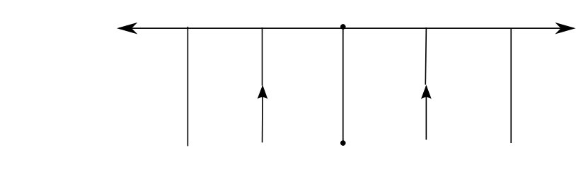 Figure 1
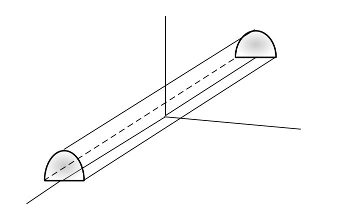 Figure 2