Preconditioning ideas for the Augmented Lagrangian method
AM Sajo-Castelli

TL;DR
This paper introduces a modular preconditioning strategy for the Augmented Lagrangian method that leverages problem structure, improves convergence, and is adaptable to various preconditioning techniques, with promising initial results.
Contribution
A novel, structure-exploiting preconditioning scheme for ALM that is flexible, efficient, and applicable to both linear and nonlinear problems, enhancing convergence without frequent updates.
Findings
Preconditioned matrices show improved spectral properties.
Numerical experiments demonstrate potential benefits on benchmark problems.
Scheme is effective for problems with few constraints relative to search space.
Abstract
A preconditioning strategy for the Powell-Hestenes-Rockafellar Augmented Lagrangian method (ALM) is presented. The scheme exploits the structure of the Augmented Lagrangian Hessian. It is a modular preconditioner consisting of two blocks. The first one is associated with the Lagrangian of the objective while the second administers the Jacobian of the constraints and possible low-rank corrections to the Hessian. The proposed updating strategies take advantage of ALM convergence results and avoid frequent refreshing. Constraint administration takes into account complementarity over the Lagrange multipliers and admits relaxation. The preconditioner is designed for problems where constraint quantity is small compared to the search space. A virtue of the scheme is that it is agnostic to the preconditioning technique used for the Hessian of the Lagrangian function. The strategy described can…
Click any figure to enlarge with its caption.
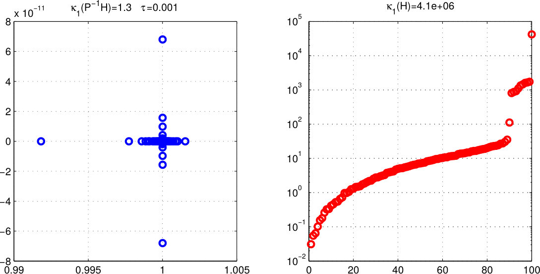 Figure 1
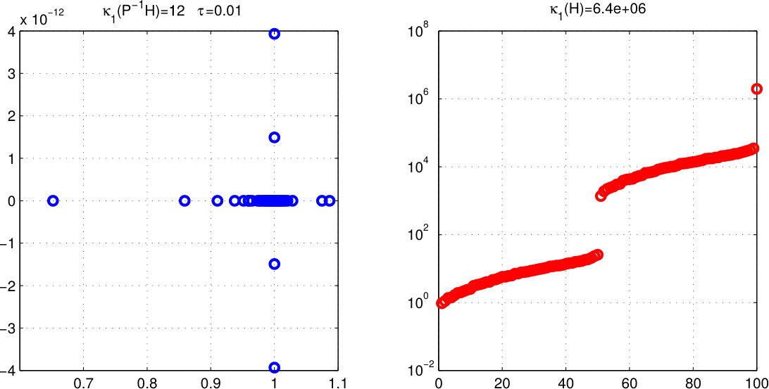 Figure 2
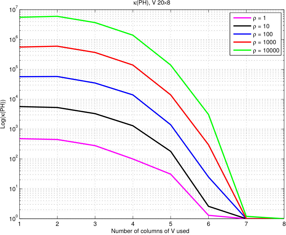 Figure 3
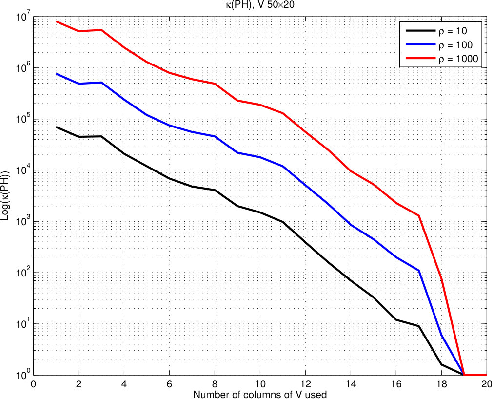 Figure 4
| 10 | 1.5 | 0.1 | ||
| 10 | 15.5 | 0.1 | ||
| 10 | 154.8 | 0.1 | ||
| 10 | 1548.3 | 0.1 | ||
| 10 | 15483 | 0.1 | ||
| 10 | 1.5 | 0.001 | 1.3 | |
| 10 | 15.5 | 0.001 | 1.3 | |
| 10 | 154.8 | 0.001 | 1.3 | |
| 10 | 1548.3 | 0.001 | 1.3 | |
| 10 | 15483 | 0.001 | 1.3 |
| Name | CG | PCG | ||||||||||
|---|---|---|---|---|---|---|---|---|---|---|---|---|
| Sparse | 1000 | 1 | 0.05 | 0.075 | 2040 | 0.002 | 0.674 | 1 | 12681509 | 74245 | n/c | 22 |
| Sparse | 1000 | 1 | 0.05 | 0.075 | 2040 | 0.002 | 0.674 | 100 | 1259615534 | 74251 | 172 | 14 |
| Sparse | 1000 | 1 | 0.05 | 0.075 | 2040 | 0.002 | 0.674 | 1000 | 12595389913 | 74251 | 58 | 9 |
| Sparse | 1000 | 100 | 0.1 | 0.1 | 1656 | 0.002 | 0.684 | 100 | 153329943 | 12 | 56 | 2 |
| Sparse | 1000 | 50 | 0.1 | 0.1 | 1666 | 0.002 | 0.684 | 1 | 2650446 | 122 | 173 | 9 |
| Sparse | 1000 | 50 | 0.1 | 0.1 | 1666 | 0.002 | 0.684 | 100 | 264040355 | 121 | 54 | 3 |
| Sparse | 2000 | 1 | 0.05 | 0.075 | 2865 | 0.001 | 0.746 | 1 | 70457448 | 70219 | n/c | 15 |
| Sparse | 2000 | 1 | 0.05 | 0.075 | 2865 | 0.001 | 0.746 | 1000 | 70285577870 | 70214 | 37 | 3 |
| bcspwr01 | 49 | 20 | 0.1 | 0.1 | 131 | 0.086 | 1 | 1 | 208 | 1.3 | 21 | 5 |
| bcspwr01 | 49 | 20 | 0.1 | 0.1 | 131 | 0.086 | 1 | 10000 | 1841063 | 1.2 | 27 | 2 |
| bcspwr01 | 49 | 1 | 0.18 | 0.18 | 142 | 0.059 | 0.85 | 1 | 171 | 15 | 31 | 17 |
| bcspwr01 | 49 | 1 | 0.18 | 0.18 | 142 | 0.059 | 0.85 | 100 | 13474 | 15 | 30 | 14 |
| bcspwr01 | 49 | 1 | 0.18 | 0.18 | 142 | 0.059 | 0.85 | 10000 | 1343884 | 15 | 21 | 9 |
| bcspwr01 | 49 | 1 | 0.18 | 0.18 | 142 | 0.059 | 0.85 | 100000 | 13438526 | 15 | 9 | 6 |
| bcspwr02 | 49 | 1 | 0.18 | 0.18 | 159 | 0.066 | 0.952 | 1 | 600 | 53 | 33 | 18 |
| bcspwr02 | 49 | 1 | 0.18 | 0.18 | 159 | 0.066 | 0.952 | 100 | 45618 | 51 | 32 | 15 |
| bcspwr02 | 49 | 1 | 0.18 | 0.18 | 159 | 0.066 | 0.952 | 10000 | 4547969 | 51 | 20 | 12 |
| bcspwr02 | 49 | 1 | 0.18 | 0.18 | 159 | 0.066 | 0.952 | 1000000 | 454783100 | 51 | 5 | 3 |
| bcspwr02 | 49 | 10 | 0.1 | 0.1 | 157 | 0.065 | 0.94 | 1 | 294 | 1.6 | 25 | 6 |
| bcspwr02 | 49 | 10 | 0.1 | 0.1 | 157 | 0.065 | 0.94 | 10000 | 2253720 | 1.4 | 27 | 2 |
| bcspwr02 | 49 | 30 | 0.1 | 0.1 | 157 | 0.065 | 0.94 | 1 | 355 | 1.3 | 21 | 5 |
| bcspwr02 | 49 | 30 | 0.1 | 0.1 | 157 | 0.065 | 0.94 | 10 | 2720 | 1.2 | 39 | 4 |
| bcsstm03 | 112 | 1 | 0.7 | 0.7 | 112 | 0.009 | 1 | 1 | 3003.3 | 1 | 42 | 1 |
| bcsstm03 | 112 | 1 | 0.7 | 0.7 | 112 | 0.009 | 1 | 1000000 | 23186836 | 1 | 19 | 1 |
| bcsstm03 | 112 | 1 | 0.7 | 0.7 | 112 | 0.009 | 1 | 10000000 | 231867364 | 1 | 7 | 1 |
| Updates | ||||||||||
| Strategy | Ext. it | Int. it | GC/MR it | Total | ||||||
| Auto | 37 | 98 | 317 | 56 | 20 | 36 | ||||
| Auto | 37 | 98 | 317 | 62 | 20 | 42 | ||||
| Auto | 37 | 98 | 317 | 62 | 20 | 42 | ||||
| Auto | 37 | 98 | 317 | 62 | 20 | 42 | ||||
| Auto | 37 | 98 | 258 | 65 | 30 | 35 | ||||
| Auto | 37 | 98 | 345 | 62 | 18 | 44 | ||||
| Auto | 37 | 98 | 345 | 62 | 18 | 44 | ||||
| Auto | 37 | 98 | 368 | 62 | 17 | 45 | ||||
| Auto | 37 | 98 | 399 | 27 | 17 | 10 | ||||
| Auto | 37 | 98 | 394 | 27 | 17 | 10 | ||||
| Auto | 37 | 98 | 373 | 65 | 17 | 48 | ||||
| Auto | 37 | 98 | 284 | 62 | 22 | 40 | ||||
| Update every external iteration | 37 | 98 | 533 | 35 | 3 | 32 | ||||
| Assemble only once | 37 | 98 | 1156 | 1 | 1 | 0 | ||||
| Newton / direct method | 37 | 98 | — | — | — | — | ||||
| L. it | N. it | PMR it (MR it) | Update type | rnnz() | ||||
| 1 | 1 | 1 (10) | MV | 10 | 100 | 1.6 | — | — |
| 1 | 2 | 1 (7) | MV* | 12 | 100 | 1.6 | ||
| 1 | 3 | 1 (5) | MV | 12 | 100 | 1.6 | ||
| 1 | 4 | 1 (5) | MV | 12 | 100 | 1.6 | ||
| 1 | 5 | 1 (5) | MV | 12 | 100 | 1.6 | ||
| 1 | 6 | 1 (5) | MV | 12 | 100 | 1.6 | ||
| 1 | 7 | 1 (5) | MV | 12 | 100 | 1.6 | ||
| 1 | 8 | 1 (5) | MV | 12 | 100 | 1.6 | ||
| 1 | 9 | 1 (7) | MV | 12 | 100 | 1.6 | ||
| 1 | 10 | 1 (8) | MV | 12 | 100 | 1.6 | ||
| 2 | 1 | 1 (10) | MV* | 10 | 100 | 1.6 | ||
| 2 | 2 | 1 (10) | MV* | 12 | 100 | 1.6 | ||
| 3 | 1 | 1 (10) | MV* | 10 | 100 | 1.6 | ||
| 3 | 2 | 1 (10) | M | 10 | 100 | 1.6 | ||
| 3 | 3 | 3 (10) | V* | 12 | 100 | 1.6 | ||
| 3 | 4 | 3 (10) | V | 12 | 100 | 1.6 | ||
| 3 | 5 | 3 (10) | — | 12 | 100 | 1.6 | ||
| 3 | 6 | 3 (10) | — | 12 | 100 | 1.6 | ||
| 3 | 7 | 3 (10) | — | 12 | 100 | 1.6 | ||
| 3 | 8 | 3 (10) | — | 12 | 100 | 1.6 | ||
| 3 | 9 | 3 (10) | — | 12 | 100 | 1.6 | ||
| 3 | 10 | 3 (10) | — | 12 | 100 | 1.6 | ||
| 3 | 11 | 3 (10) | — | 12 | 100 | 1.6 | ||
| 3 | 12 | 3 (10) | — | 12 | 100 | 1.6 | ||
| 3 | 13 | 3 (10) | — | 12 | 100 | 1.6 | ||
| 3 | 14 | 2 (10) | — | 12 | 100 | 1.6 | ||
| 3 | 15 | 2 (10) | — | 12 | 100 | 1.6 | ||
| 3 | 16 | 2 (10) | — | 12 | 100 | 1.6 | ||
| 3 | 17 | 2 (10) | — | 12 | 100 | 1.6 |
| Name | Method | ItL. | Itin | Itpd | Itd | AcM | AcV | Time (s) | ||
| C4-1 | 10 | 10 | NW | 11 | 52 | 82 | 420 | 35 | 1 | 2.4 |
| C4-1 | 10 | 10 | NW | 10 | 53 | 83 | 432 | 34 | 2 | 2.5 |
| C4-1 | 10 | 10 | QN | 45 | 143 | 311 | 1365 | 40 | 19 | 5.7 |
| C4-1 | 10 | 10 | QN | 45 | 143 | 176 | 1365 | 107 | 6 | 5.9 |
| C4-R-10 | 10 | 10 | QN | 3 | 29 | 55 | 252 | 14 | 2 | 1.0 |
| C4-R-20 | 20 | 10 | QN | 3 | 48 | 265 | 617 | 33 | 6 | 1.6 |
| C4-R-25 | 25 | 10 | QN | 4 | 55 | 112 | 900 | 37 | 18 | 1.7 |
| BT3 | 5 | 3 | NW | 8 | 84 | 84 | 807 | 1 | 3 | 1.3 |
| BT3 | 5 | 3 | NW | 7 | 86 | 86 | 539 | 1 | 1 | 1.4 |
| BT3 | 5 | 3 | QN | 8 | 129 | 182 | 651 | 21 | 58 | 1.8 |
| BT3 | 5 | 3 | QN | 8 | 129 | 193 | 651 | 20 | 50 | 1.7 |
| BT8 | 5 | 2 | NW | 5 | 72 | 87 | 148 | 27 | 0 | 1.1 |
| BT8 | 5 | 2 | QN | 5 | 88 | 108 | 169 | 26 | 8 | 1.3 |
| BT11 | 5 | 3 | NW | 10 | 140 | 322 | 707 | 38 | 4 | 2.1 |
| BT11 | 5 | 3 | NW | 8 | 114 | 134 | 680 | 112 | 0 | 1.8 |
| Name | Method | ItL. | Itin | AcM | AcV | Time (s) | ||
| C4-1 | 10 | 10 | SG | n/c | — | — | — | — |
| C4-1 | 10 | 10 | PSG | 1 | 21 | 3 | 0 | 0.3 |
| BT3 | 5 | 3 | SG | 9 | 486 | — | — | 1.6 |
| BT3 | 5 | 3 | PSG | 7 | 19 | 12 | 0 | 0.4 |
| BT8 | 5 | 2 | SG | 3 | 29 | — | — | 0.3 |
| BT8 | 5 | 2 | PSG | 3 | 17 | 5 | 0 | 0.3 |
| BT9 | 4 | 2 | SG | 9 | 193 | — | — | 0.8 |
| BT9 | 4 | 2 | PSG | 9 | 32 | 25 | 0 | 0.5 |
| BT11 | 5 | 3 | SG | 7 | 426 | — | — | 1.5 |
| BT11 | 5 | 3 | PSG | 7 | 28 | 28 | 0 | 0.4 |
| BT12 | 5 | 3 | SG | 7 | 1222 | — | — | 4.3 |
| BT12 | 5 | 3 | PSG | 6 | 16 | 12 | 0 | 0.3 |
| HS48 | 5 | 2 | SG | 2 | 131 | — | — | 0.5 |
| HS48 | 5 | 2 | PSG | 1 | 2 | 2 | 0 | 0.2 |
| MAKELA4 | 21 | 40 | SG | 2 | 5 | 0 | 0 | 0.1 |
| MAKELA4 | 21 | 40 | PSG | 2 | 3 | 3 | 0 | 0.3 |
| Name | Method | ItL. | Itin | AcM | AcV | Time (s) | ||
| AIRPORT | 84 | 42 | SPG | n/c | — | — | — | — |
| AIRPORT | 84 | 42 | PSPG | 81 | 304 | 159 | 0 | 18.9 |
| AIRPORT | 84 | 42 | PSPG | 81 | 304 | 159 | 0 | 22.9 |
| EXTRASIM | 2 | 1 | SPG | 1 | 16 | — | — | 0.2 |
| EXTRASIM | 2 | 1 | PSPG | 1 | 2 | 2 | 0 | 0.2 |
| HS41 | 4 | 1 | SPG | 4 | 78 | — | — | 0.4 |
| HS41 | 4 | 1 | PSPG | 4 | 78 | 6 | 0 | 0.7 |
| HS63 | 3 | 2 | SPG | 4 | 125 | — | — | 0.5 |
| HS63 | 3 | 2 | PSPG | 4 | 26 | 16 | 0 | 0.5 |
| HS90 | 4 | 1 | SPG | 1 | 10 | — | — | 0.1 |
| HS90 | 4 | 1 | PSPG | 1 | 8 | 1 | 0 | 0.2 |
| HS105 | 8 | 1 | SPG | 2 | 505 | — | — | 4.5 |
| HS105 | 8 | 1 | PSPG | 1 | 100 | 82 | 0 | 2.1 |
| HS105 | 8 | 1 | PSPG | 1 | 80 | 49 | 0 | 1.7 |
| HS111 | 10 | 3 | SPG | 12 | 5999 | — | — | 21.7 |
| HS111 | 10 | 3 | PSPG | 12 | 56 | 41 | 0 | 0.8 |
| HS111 | 10 | 3 | PSPG | 12 | 86 | 36 | 0 | 1.2 |
| HS112 | 10 | 3 | SPG | 12 | 1567 | — | — | 5.7 |
| HS112 | 10 | 3 | PSPG | 12 | 37 | 35 | 0 | 0.8 |
| LOOTSMA | 3 | 2 | SPG | 1 | 34 | — | — | 0.6 |
| LOOTSMA | 3 | 2 | PSPG | 1 | 34 | 1 | 0 | 0.5 |
Peer Reviews
No public reviews on file for this paper yet. If you reviewed it on a platform where reviews are public (OpenReview, ICLR, NeurIPS, ICML), you can paste yours below so the community can read it here.
Videos
No videos yet. Explain this paper in a talk, walkthrough, or lecture? Add one.
Taxonomy
TopicsMatrix Theory and Algorithms · Advanced Numerical Methods in Computational Mathematics · Advanced Optimization Algorithms Research
Preconditioning ideas for the Augmented Lagrangian method
A. M. Sajo-Castelli
Departamento de Cómputo Científico y Estadística, Universidad Simón Bolívar, Ap. 89000, Caracas 1080-A, Venezuela.
(December 16, 2016)
Abstract
A preconditioning strategy for the Powell-Hestenes-Rockafellar Augmented Lagrangian method (ALM) is presented. The scheme exploits the structure of the Augmented Lagrangian Hessian. It is a modular preconditioner consisting of two blocks. The first one is associated with the Lagrangian of the objective while the second administers the Jacobian of the constraints and possible low-rank corrections to the Hessian. The proposed updating strategies take advantage of ALM convergence results and avoid frequent refreshing. Constraint administration takes into account complementarity over the Lagrange multipliers and admits relaxation. The preconditioner is designed for problems where constraint quantity is small compared to the search space. A virtue of the scheme is that it is agnostic to the preconditioning technique used for the Hessian of the Lagrangian function. The strategy described can be used for linear and nonlinear preconditioning. Numerical experiments report on spectral properties of preconditioned matrices from Matrix Market while some optimization problems where taken from the CUTEst collection. Preliminary results indicate that the proposed scheme could be attractive and further experimentation is encouraged.
keywords:
Augmented Langrangian Method, Preconditioning, Iterative methods.
MSC:
65F10, 15A12, 65F35, 90C30, 90C25.
1 Introduction
Augmented Lagrangian methods (ALM) are practical and affordable algorithms extensively used in applied fields. They are designed to solve large-scale nonlinear optimization problems possibly with nonlinear constraints. The constraints are classified in two groups: hard and soft. Hard constraints are such that strict fulfillment is required in order to accept a solution while minor infeasibility for the soft constraints is granted. Birgin and Martínez in [1] present a recent and detailed overview of practical ALM. These methods are considered a general optimization machinery [2, 3, 4, 5, 6, 1, 7] in the sense that they successfully cope with a great variety of real-life problems. ALM has also been adapted to very specific applications [8, 9, 10]. A great virtue of the method is that it can be accelerated via preconditioning techniques.
Iterative Krylov-type methods have been used inside ALM and even though they are very well studied and can handle very large-scale problems, it is well known the poor convergence speed. Accelerating these methods by preconditioning strategies is common practice. In the last 50 years a considerable amount of effort has been invested in the design and construction of effective preconditioners. In the context of ALM, there has not been much motivation to study acceleration strategies that benefit or exploit convergence results, although recently some studies on very special problems present non-induced preconditioning that benefit from ALM convergence [11, 12, 13].
State of the art ALM implementations that can be highlighted are Algencan [1, 3, 4] and Lancelot B [14, 15]. Both are considered production-grade codes that use a variety of direct and iterative methods, such as the Conjugate Gradients method. In regards to acceleration, Algencan does not offer enough flexibility while Lancelot B incorporates a list facilities, it can also leave to the user the task of administering the whole preconditioning process. Surely this last option covers all possible scenarios, but it can also be daunting for non-expert users. From the user-land perspective, these MLA implementations leave a certain void preconditioning-wise. The proposed acceleration scheme tries to fill this gap.
In this work we present a modular acceleration scheme that exploits the special structure of the Augmented Lagrangian of Powell-Hestenes-Rockafellar. A key aspect is that the update strategies take advantage of ALM convergence. The scheme has two main ingredients, an auxiliary preconditioner associated with the Lagrangian function and a machinery that administers the constraints. Separating these components has the great advantages of freedom in choosing the auxiliary preconditioner and having full control over the Jacobian matrix of the constraints and possible low-rank corrections. Such corrections are attractive because they promote quality in the approximation to the Hessian of the Lagrangian function. The proposed scheme is considered a generalization of the qncgna preconditioner used in Algencan [16, 1].
The rest of this document is organized as follows. We briefly introduce the problem of interest and the Augmented Lagrangian Method followed by the presentation of the acceleration scheme. The preconditioner is introduced in two parts. We start by showing how to accelerate ALM for problems with a single constraint, then a general preconditioner is presented. Update strategies for the various components are discussed and some illustrative numerical results are reported. The work concludes with some final remarks.
2 The Augmented Lagrangian Method
Let us consider the following optimization problem
[TABLE]
where , , are continuous functions, in particular is two times continuously differentiable and . With the goal to solve (1), two functions are associated, the Langrangian
[TABLE]
where y are the Lagrange multipliers of the problem, and the Augmented Lagrangian of Powell-Hestenes-Rockafellar [17, 18]
[TABLE]
with the external penalty parameter , y . Taking the Augmented Lagrangian function as the objective, then solving (1) and minimizing (3) with respect to , are equivalent problems. The ALM consists of solving a sequence of sub-problems and updating the the Lagrange multipliers and the external penalty parameter as required. This naturally divides the iterations in two groups, external or Lagrangian iterations and internal iterations. On the external iterations the multipliers and the penalty parameters are updated while the internal iterations are dedicated in solving the sub-problem. Soft constraints are moved up to the objective penalizing a shifted version of infeasibility measure. Hard constraints are enforce inside the inner solver which is dedicated to the sub-problem
[TABLE]
where , and are fixed.
The ALM is conceptually presented in Algorithm 1. The algorithm is schematic and leaves open the choice on how to solve the sub-problem (4), it only requires that be an approximate solution. On each external iteration (Step 4) it is considered if has done enough progress in regards to feasibility and complementarity. In cases where progress is good, the external penalty parameter does not need to change, on the contrary the parameter must be incremented. The idea behind the shifts and is that even when the external penalty parameter has a moderate penalty, there can exist adequate values for the shifts on the multipliers where it is possible to find an acceptable solution to (4). Given the interest of the algorithm to produce a numerically attractive result, on Step 5 the multipliers are safeguarded.
We briefly present convergence results for Algorithm 1, details and theorem proofs are given in [1, Chapter 5]. For the following results it is assumed that on Step 1 of Algorithm 1, is a global minimizer of (4):
[TABLE]
where is bounded and need not be small.
Theorem 1** (Feasibility)**
Let be a sequence generated by Algorithm 1 under the previous assumption and let be a limit point of this sequence. Then,
[TABLE]
This result guarantees that if the problem is feasible, then every limit point of the sequence generated by ALM is also feasible.
Theorem 2** (Optimality)**
Let be a sequence generated by Algorithm 1 and be a limit point of . Suppose that and that the problem (4) is feasible. On Step 4, when possible, is not incremented. Then, is a global minimizer.
For practical purposes it is not necessary to differentiate between the equality and inequality constraints, they can be both considered under the umbrella constraint function and the associated multiplier vector . Optimality conditions and constraint handling requires only minor attention. The Augmented Lagrangian becomes
[TABLE]
where the sets and contain the indexes of equality and inequality constraints respectively.
Supposing that problem (1) has solution, then the pair is minimizer of (5) —and in consequence is also of (3) and solution to (1)— when it satisfies
[TABLE]
where
[TABLE]
The operator is the Euclidean projection on the convex set . Conditions (6) and (7) insure that is a stationary point of the problem while condition (8) guarantees that the point satisfies the required feasibility tolerance.
It is advantageous to differentiate between Lagrangian and internal iterations. External iterates and counter are identified by and respectively while internal ones use and respectively. If the set then the sub-problem is said to be unconstrained, on the contrary it will be assumed to be convex constrained.
Practical Newton-type methods are very popular for solving unconstrained problems and require a descent direction of first order given by solving the quadratic model
[TABLE]
where is the Hessian or an approximation to it. For the Truncated-Newton method, is estimated using the Conjugate Gradients method in the SPD case or Minimal Residual method when is symmetric but undefined. These methods are quite attractive if accelerated with high quality preconditioners.
Practical solvers for convex constrained problems are the Spectral Projected Gradient method (SPG) [19, 20, 21] and its preconditioned variant (PSPG) [22]. PSPG has received some attention [23] and can be viewed as a nonlinear preconditioned variant that combines the Preconditioned Spectral Gradient method and SPG. For these type of problems we assume that is the Euclidean projection operator over the convex set , exists and is of acceptable cost. We also require that the first order derivatives of and exist wherever required.
3 Preconditioning ideas
Under our context, accelerating ALM may refer to accelerate the resolution of the sub-problem (Newton-type directions) as well as the acceleration for the estimation of the descent direction (Cauchy-type machinery). Given the nature of the method to solve at each external iteration an optimization problem, and that the sequence of these problems tend to be similar, preconditioning schemes must recycle between iterations in order to be attractive.
In order to propose preconditioning schemes for (4), it is necessary to study the explicit form of the Hessian of the objective (Augmented Lagrangian function). For historical reasons, most applications use and implement the Lagrangian function and not its augmented counterpart. Although, as we shall see both are closely related. The Lagrangian function, gradient and Hessian associated to (5), are
[TABLE]
On the other hand, the Augmented Lagrangian counterpart is
[TABLE]
Noting that , we obtain the key identity
[TABLE]
This matrix sum has many relevant characteristics. For instance, since is the sum of Hessian matrices it is symmetric and close to a solution is definite [24]. Under certain choices of , it can be verified that it is always definite [6]. The Gauss-Newton matrix is always symmetric and can be regarded semi-definite. Moreover, if then the rank of is at best , the number of soft constraints. In practice, methods exploit the complementary condition in such a way that the rank of is at most the number of active non-relaxed constraint count at current iterate.
When solving problem (4) using Newton-type directions, it is necessary to solve the quadratic model
[TABLE]
For Cauchy-type directions, if is a preconditioner for , then we interpret the preconditioner as an approximation to and the enriched descent direction is
[TABLE]
Contrasting the previous two expressions, applying nonlinear preconditioning for Gradient-type methods fortunately is analogous as accelerating the Newton-type machinery. Our interest lies in solving the linear system (9) using Krylov-type iterative methods, PCG when is PD or MinRes for the undefined case. Preconditioning schemes for ALM must be able to at least exploit the following two desirable key features:
Preconditioner recycling. The idea is to take advantage of convergence for the sub-problems. Supposing that (1) has solution, then we expect , meaning that starting from a certain iterate (or ) it is possible to bound the difference and successfully use the same preconditioner onwards. 2. 2.
Preconditioner update. Assembly of should partially reuse work invested in assembling . Generally speaking this is not straightforward. As an illustrative example on the involved difficulties, low-rank updates [25, 16, 26, 27, 28] are highlighted with special focus on BFGS-type corrections [29, 30].
In what follows we propose a new preconditioning scheme that takes advantage of these features.
3.1 Preconditioning singly constrained sub-problems
Many applications can be modeled using singly constrained problems: support vector machine formulations for classification or pattern recognition [31, 32] are but two mainstream examples. This subsection introduces a new inverse preconditioner scheme for solving the following singly constrained problem
[TABLE]
We simplify notation by relaxing the index from the constraint and its associated Lagrange multiplier. With the idea to introduce the preconditioner, suppose a Newton-type machinery is used to solve (10), then at each internal iteration it is required to find from the linear system
[TABLE]
with
[TABLE]
Relaxing the iteration indexes, we have
[TABLE]
where is considered a non-null vector, is a rank-1 matrix and we suppose is full rank. Given our interest in solving (11) using PCG or MinRes, applying the preconditioner [24, Algorithm 5.3: line 3 and equation (5.38d)] reduces to efficiently compute the product
[TABLE]
The matrix in (11) is special in the sense that it is the sum of an invertible matrix plus a rank-1 matrix. Suppose that is precisely H^{-1}=\Big{[}M+\rho\,vv^{\operatorname{\mathsf{T}}}\Big{]}^{-1}\!\!\!\!\!,\;\; then the product can be computed using the Sherman-Morrison identity [33],
[TABLE]
solving for , or , we obtain
[TABLE]
analogously we find , or and observing that is a scalar, we finally have
[TABLE]
If is not trivially invertible, finding and requires an auxiliary preconditioner . Each form of obtaining and consequently , give rise the different preconditioning strategies. It is noteworthy to remark that the preconditioner is never assembled and is considered an abstract preconditioner which relies upon the auxiliary preconditioner . This highlights the agnostic nature of , for it does not enforce any specific choice over . Under this scheme, the spectrum of the preconditioned matrix P^{-1}\big{[}M+\rho\,vv^{\operatorname{\mathsf{T}}}\big{]} is described by the following result.
Theorem 3
Suppose is the Hessian matrix of the Lagrangian function associated to (10), let the preconditioner for be P=\big{[}M+\rho\,vv^{\operatorname{\mathsf{T}}}\big{]}, furthermore let be a preconditioner for , and , then the spectrum of is
[TABLE]
The proof of this theorem can be found in [34]. This result has a few important implications. If , then This indicates that for very large values of it is not attractive or even necessary to precondition. It also shows that the condition of can be described in terms of , this is to say that the quality of is given in direct relation to the quality of .
3.2 General Preconditioner
In this section we work with the problem
[TABLE]
where the quantity of constraints is less than the problem dimension. Analogous to (11), the linear system to solve is
[TABLE]
where is the constraint Jacobian, is the Gauss-Newton matrix of rank at most and we suppose that is rank complete. Initially, we set the preconditioner to P^{-1}=\Big{[}M+\rho VV^{\operatorname{\mathsf{T}}}\Big{]}^{-1}. The use of the Sherman-Morrison-Woodbury [35, 36] inverse closed formula rises many difficulties, specially the stringent requirement of a composed matrix inverse which for our case is not practical. Fortunately, can be rewritten as a recursion over the columns of , suppose (12) has three constraints (), then
[TABLE]
This formulation shows that can always be written as an invertible matrix plus a rank-1 matrix. This is also true for the preconditioner , let , then
[TABLE]
which leads to the following recursion,
[TABLE]
Using Miller’s inverse formula [37], the product is reduced to the recursion
[TABLE]
but this was previously shown how to be solved, and is
[TABLE]
Implementation-wise, the are computed at the same time as the which leads to a secondary recursion.
Although the previous formulation requires double recursion over the columns of , it will be shown to have many attractive features. The elements , and finally the acceleration product , are computed by applying multiple times the Sherman-Morrison identity. This is considered a very attractive aspect because it only requires Matrix-Vector and internal products.
In the same spirit as the single constrained case, each form of obtaining and give rise to different preconditioners and this variant is also considered to be an agnostic acceleration scheme which leaves open the strategy on how to estimate and . This has numerous advantages, we highlight the fact that handling the Lagrangian independently from the constraint Jacobian permits to exploit the sparse structure of the problem.
In the next section we generalize the previous example of three constraints.
3.2.1 The Matrix
Observing the recursion that computes the product (13), it can be seen that elements and do not depend on but on the columns of . This in a natural way induces to pre-compute and , and save them efficiently in a storage matrix. In what follows we show how to efficiently compute the product .
Let , where indicates the -th column of matrix .
On a first pass, storage matrix is assembled,
[TABLE]
Finally . It is important to note that from the implementation point of view, the elements of overwrite those of in such a way as not to waist storage. The recursion to compute distills to
[TABLE]
where regains its classical meaning indicating the -th column of . Storage matrix unites in a single matrix all the ingredients to estimate and as such it is intimately related to and . The previous formulation efficiently computes the product or for any as long as and stay relatively the same. Significant changes in and/or force re-assembly of . This fact outlines certain updating aspects that an acceleration scheme must be aware of. It is evident that this strategy to compute is only attractive when is far from . The proposed preconditioner can be shown trivially that is adequate for use within PCG and MinRes.
3.2.2 Secant type directions
In large-scale applications computing the Augmented Lagrangian Hessian is a luxury seldom available, in general terms a reasonable approximation is used. Within our context, the Augmented Lagrangian Hessian has clear differentiation between its components
[TABLE]
Krejić et al. [6] propose using and Birgin and Martínez suggest in [1] to use only along with two corrections. These involve a spectral correction [38, 39, 19, 40] using the associated Rayleigh quotient [41, 42] and a second correction [16, 1] in the spirit of BFGS that forces to satisfy the Secant equation [27, 26]
[TABLE]
These corrections are low-rank [28, 43, 44, 30, 45, 46] and are crafted with the main purpose of having a closed inverse form. For illustrative purposes, is corrected spectrally and with the famous BFGS formula,
[TABLE]
Now, if , the assembly and use of the preconditioner is analogous as shown at the start of §3.2 since can be rewritten as an invertible matrix plus matrices of rank-1. Let us see,
[TABLE]
That is, has the form required to assemble . The matrix is guaranteed to be rank complete by means of the first spectral correction. With some abuse of notation, the constraint Jacobian is augmented to accommodate the elements associated with the BFGS correction
[TABLE]
The auxiliary vector “signs” is used inside the recursion associated with .
3.2.3 Special Exact Case
When using Quasi-Newton directions, the choice of the approximation to the Lagrangian Hessian plays a key role in determining the quality of the auxiliary preconditioner associated to . If the election of that approximates has explicit inverse, then is the exact (theoretical) inverse of . A trivial case is to choose diagonal. As a side-effect under this context, the proposed preconditioner can be seen as a generalization of the qncgna preconditioner of Birgin and Martínez [16, 1]. The preconditioner is designed to work on the linear system
[TABLE]
The matrix is symmetric and SPD, it is corrected spectrally and, if possible, a second BFGS-style correction is applied. The corrected approximation to the Augmented Lagrangian Hessian is
[TABLE]
and the qncgna preconditioner
[TABLE]
Witch has explicit closed inverse
[TABLE]
Note that the search direction is done over and the preconditioner is over \operatorname{{\mathrm{diag}}}\!\big{(}V\!(z)\big{)}.
Now taking up (16), the matrix can be rewritten as a rank complete matrix plus the sum of rank-1 matrices. Suppose the BFGS correction is possible, then
[TABLE]
Let and —again, with some notation abuse— be the matrix of size that gathers the constraint Jacobian and the vectors associated with the second BFGS correction, then defining trivially we have that is the explicit closed inverse of .
3.3 Update Strategies
There exist a variety of updating choices for the preconditioner within ALM. Given the available granularity inside the recursive nature of applying the preconditioner (), update strategies enjoy a fine-grain control over each component. Practical update strategies monitor changes on \big{\|}M_{\ell}-M_{\ell-1}\big{\|} and \big{\|}V_{\ell}-V_{\ell-1}\big{\|} independently and take the following actions:
Update whenever \big{\|}M_{\ell}-M_{\ell-1}\big{\|}_{1}>\delta_{M}. 2. 2.
Update each time \big{\|}V_{\ell}-V_{\ell-1}\big{\|}_{1}>\delta_{V} or \big{\|}M_{\ell}-M_{\ell-1}\big{\|}_{1}>\delta_{M}. 3. 3.
Apply relaxation over the columns of when assembling or at the moment of applying the preconditioner (). This can be done by using only those columns of that in norm are greater that a threshold or that have huge infeasibility measure, V=(v_{i}),\;i=1:m\;\;\big{|}\;\;\|v_{i}\|>\varepsilon_{v}>0\;\vee\;i\in{\mathbb{E}}\;\;\big{|}\;\;|\operatorname{\mathrm{c}}_{i}(x)|>\varepsilon_{c}>0\;\vee i\in{\mathbb{I}}\;\;\big{|}\;\;\big{(}\operatorname{\mathrm{c}}_{i}(x)\big{)}_{+}>\varepsilon_{c}.
The idea behind the first item is that if and are similar, then possibly will also be a good preconditioner for . Item two establishes that should only be updated if and greatly differ. It also forces an update if was updated. Up until not finding the final search space, will be changing drastically and update schemes must be aware of this. The last item is based on the idea that small elements should have small contributions and can be safely discarded.
3.3.1 Strategies for
The proposed scheme leaves open the choice on how to precondition . Clearly the updating of depends on such choice. Nevertheless some maintenance aspects of can be mentioned. The update of should be delayed as much as possible due to the fact that updates on force an update on . A great advantage on the modularity of is that it allows among other things, to change preconditioning strategy () mid-way between two updates.
Preliminary experimentation shows that most of the big changes for \big{\|}M_{\ell}-M_{\ell-1}\big{\|}_{1} occur at the beginning and specially between two external iterations due to the Lagrangian multipliers and the external penalty parameters being updated. Given the convergence of ALM and supposing the problem has solution, iterates will converge asymptotically to a point where updating will no longer be necessary. The reported experiments suggest to use a lax threshold for the update of . This choice promotes frequent updates only at the beginning of the resolution while avoiding unnecessary updates towards the end.
3.3.2 On the update of matrix
Matrix is associated with the constraint Jacobian and as such its form is described by the active non-relaxed constraints and the rank-1 correction artifacts. Given the recursive nature of the assembly of , it is possible to establish predictive update strategies that reduce costs. The idea is the following. Let be the second to last column of and the gradient associated with the inequality constraint and also suppose that it has a very small infeasibility measure. Most probably the next iterate will inactivate this constraint forcing the discarding of . This induces and update only to the last two columns of . Now, if where to be the first column of then the induced update would affect all the columns of having a much greater cost. This observation suggest orderings over the columns of that potentially reduce the cost of updating . A practical ordering could be induced by the infeasibility measure of each constraint
[TABLE]
The spirit behind this ordering is to leave for the end of the recursion those columns whose associated constraints will (possibly) soon be discarded. This ordering could be further improved by taking into account the norm of each associated gradient. It is also very convenient to leave at the end of the recursion the columns associated with BFGS-type corrections. These elements can have a vivid transit state since initially iterations may or may not fulfill the condition Although, it has been observed that close to a solution the BFGS correction can always be applied. Numerical experimentation shows that as iterates approach a solution, changes in diminish down to a point where updating is not necessary and can be recycled successfully.
3.4 Comments
Accelerating Cauchy-type methods require to consider preconditioning matrices as approximations to the inverse of the Hessian. Acceleration enriches the descent direction with second order information from the approximation of . In others words, the enriched direction is obtained by solving
[TABLE]
but this is exactly the same task as applying acceleration under Newton-like choices. Hence the instructions on how to apply and when to update the (linear) preconditioner are analogous for the nonlinear case. Unfortunately the enriched (preconditioned) direction is not always a descent direction. In these cases, the enriched direction is discarded in favor of , albeit, the work invested in building the approximation should not be discarded: it could potentially be recycled the next time an enriched direction is to be computed.
The assembly and maintenance of matrix loses appeal and stops being attractive in the presence of a large number of active constraints, say or even . In this scenario, we have where is dense and possibly rank complete or near complete. As iterates start closing-in to a solution, the number of active constraints should decrease down to a point where the use of is practical. This suggest to handle acceleration for problems with a large amount of constraints in a two-stage approach.
A possible heuristic is to use Quasi-Newton directions induced by where is the set of constraints indexes for the elements with greatest infeasibility measure. The quadratic model for the direction is
[TABLE]
Under these two choices, it is possible to use the proposed scheme. It is important to note that before finding the final search space, the set will be changing inducing unfavorable frequent updates on matrix .
It is important to consider alternative techniques that do not use the explicit form of the constraint Jacobian but can tackle with the dense Gauss-Newton matrix . This topic is considered open for future study.
4 Numerical Experiments
All experiments were run using Matlab® R2012a on an Intel® Core™ i7-2640M CPU @ 2.80GHz with 8 GB of memory. We start by examining the quality of as a preconditioner for and its efficiency at solving linear systems of the form . Some experiments involving constraint relaxation and preconditioner update strategies follow. We finalize by solving unconstrained and box-constrained problems from the CUTEst[47] data-set.
4.1 Spectral Properties of the Preconditioned Matrix
We wish to understand the spectral properties of the preconditioned matrix P^{-1}H=P^{-1}\big{[}M+\rho\,VV^{\operatorname{\mathsf{T}}}\big{]}. Quality metric is based on condition number and spectra of . For these experiments, the auxiliary preconditioner is of the family of Robust Incomplete Factorization of type SAINV [48, 49, 50, 51] and is considered a black-box that executes the matrix-vector product . Table 1 and Figure 1 report two particular experiments on sparse random matrices of size 100 with random constraints. These experiments use a diverse range of values for the external penalty and dropping parameters.
From the table and figure it can be observed that the higher the quality of (smaller ) the spectrum of accumulates around the identity, albeit, if is poor then the conditions of and are comparable. Curiously for these problems, higher values of seem to have a favorable effect over the condition of . Increased values of worsen the condition of while promoting the one of .
The next set of experiments involve solving the linear system of equations with using the Conjugate Gradients method. Tested matrices are sparse random and from the Matrix Market [52] collection. All matrices are forced to be real SPD. Constraints are random with N() distribution. Convergence tolerance is set to . Obtained result are reported in Table 2. Dropping parameters y are associated with . Column labeled with “” represents the number of constraints and the columns associated with give an idea of the density of . Columns “CG” and “PCG” report the number of iterations required. From the table an evident influence of over the conditioning of is observed. The higher the quality of , the more evident is the acceleration. On some problems, for very large values the number of CG iterations is surprisingly low and preconditioning stops being practical. Conversely, in some cases where is very ill conditioned, preconditioning not only is very effective but is the only alternative that converges. In PCG context, increment in generally implies reduction in iteration count.
4.2 Constraint Relaxation & Update
Updating the preconditioner on each iteration is prohibitively expensive and even unnecessary. The convergence of ALM guarantees that sub-problems will tend to be similar up to the point where recycling the preconditioner is possible. For inequality constraints, as soon as the iterate is feasible or strongly feasible, the number of active constraints drops drastically. This leads to propose cheap update strategies that discard elements from the matrix. Active constraint relaxation must be done with certain care. Preliminary experiments suggest it is not easy to establish the contribution of each active constraint to the Gauss-Newton matrix. With the idea of understanding the influence of each constraint (column of ) on the quality of the preconditioner , spectral properties of are monitored while assembling with a sub-set of columns of . For these experiments can be considered . Preconditioner is assembled by increasing the amount of columns of included. The order of inclusion is given by the norm of each column, . Figure 2 shows the condition number of in function of and the number of columns of used in the assembly of . Poor behavior can be observed, in order to maintain good quality most of the components of must be used. Attractive relaxation strategies have to account at least for the norm and infeasibility measure of the components of . This suggests to assemble using only those active constraints where and .
Updating strategies for must take advantage of the convergence of ALM. At first changes to and are assumed to be big but will tend to smooth as the sub-problems start to be similar. In order to understand the associated costs of diverse updating strategies for , the following experiments are conducted. Let and be updating tolerances for changes in matrices and between two consecutive iterations. We solve problem C4 [34] varying parameters , , (relaxation on ) and (dropping tolerance for ), while observing the amount of updates required to produce a solution. Table 3 reports a sequence of experiments on problem C4 to understand updating strategies/cost relation. The cost of each configuration is given by CG/MinRes iterations and the amount of updates on and required to find a solution. These two counters are antagonistic. In general terms, low CG/MinRes iteration count corresponds to a high update count for and . The idea is to find a compromise between these two. Reported numerical results in Table 3 give an intuitive overview of attractive configurations.
Table 4 shows in detail the dynamics of certain parameters while solving problem C4 using QN machinery. The problem is rigged to have ten variables with nine inequality and one equality constraints. Descent direction is found using MinRes. The auxiliary preconditioner is ILU of type Crout with dropping tolerance . Column labeled “Update type” specifies the three reasons for updating : “M” and “V” indicate that changes between two consecutive or matrices where greater that and/or respectively, while “V*” indicates a forced update to due to BFGS-style corrections ( changes from 10 to 12). It can also indicate that the correction cannot be applyed in the current iteration ( changes from 12 to 10). indicates the quantity of columns of matrix in use and rnnz() indicates the density of relative to . From Table 4 it can be observed that initially the changes between two consecutive matrices and are substantial, hence the update type “MV”. Further in the resolution of the problem, changes to start to attenuate then diminish for . In general terms, this behavior ca be considered characteristic. In particular, for problem C4 after iteration 4 of Lagrangian iteration 3 it was no longer necessary to update which represents a 44.8% reduction in unnecessary updates.
Obtained results show the convenience of updating via and tolerances over strategies that update on predefined iterations e. g. every Lagrangian iteration. Unfortunately, experimentation showed that attractive update tolerances is problem dependent and requires individual adjustment. For some problems these can be lax and still give good acceleration results, specially for changes between elements of . It is also attractive to relax the small columns of since it potentially reduces costs and can efficiently be controlled using a single additional relaxation parameter. Adding and removing columns from is a frequent task. This requires cheap machineries that handle efficiently the addition and removal of elements within the matrix . Furthermore, the assembly order inside of can take advantage of a prediction ingredient based on constraint gradient size and infeasibility measure.
4.3 Unconstrained Sub-problems
In each Lagrangian iteration, the problem to solve is
[TABLE]
Two type of quadratic models where used for the direction. Newton (NW) and Quasi-Newton (QN)
[TABLE]
where is the set of active non-relaxed constraints indexes, the inverse Rayleigh quotient and BFGS represents rank-one corrections. The auxiliary preconditioner used is from the ILU family. Table 5 reports the obtained experimental results. Acceleration is evident when contrasting columns labeled “Itpd” and “Itd”. For this set of problems, the preconditioning scheme achieved acceleration factors between 1.3 and 9.6.
On some problems the QN direction did not converge. Most of the computational effort is invested in updating , this promotes approximations to that are easy invertible, such as band-diagonal approximations. Preconditioners used in the NW and QN models are also used in the Spectral Gradient method (SG)111SPG code adapted from the TANGO project [19, 20]. and its preconditioned variant (PSG). Comparing the column “Itin” of the rows “SG” and “PSG” for each problem in Table 6 acceleration in iteration count is evident, but if comparing computational cost, preconditioning is not always attractive.
4.4 Box-constrained Sub-problems
For these experiments, the problem to solve is
[TABLE]
In order to understand the efficiency of the scheme, the sub-problems are solved using SPG and its preconditioned variant PSPG. Table 7 reports numerical experiments, similar results to Table 6 were obtained. Acceleration is clear when applying the preconditioner (HS105, HS111 y HS112). In some problems using the preconditioner reduces iteration count but increments overall cost (EXTRASIM, HS41 y HS63). This last aspect indicates that fine-tuning is required in order to avoid premature activation of the preconditioner. Premature activation of does not increase total iteration count but does have a negative impact of overall computational cost. The idea is to find a compromise between updating too frequently and iterating a large amount of times. A conservative strategy would be to delay the activation of the preconditioner up until the iterates are close to a solution. Another alternative could be to activate preconditioning as soon as the iterates start to be very feasible thus promoting the acceptance of the preconditioned direction.
5 Concluding remarks
An acceleration scheme for the Augmented Lagrangian method was presented. The associated preconditioner () exploits the explicit form of the Augmented Lagrangian Hessian () without estimating its inverse. The strategy is modular and uses two main ingredients. An auxiliary preconditioner () associated with the Lagrangian Hessian () and a storage matrix () related to the constraints Jacobian matrix and possible rank-one corrections of . The preconditioner takes inspiration in the Sherman-Morrison identity and Miller’s inverse formula. A virtue of this scheme is that the acceleration strategy is agnostic to the class of preconditioner used for . For special choices of approximations to the Lagrangian Hessian, the preconditioner is the exact inverse. Quasi-Newton and Secant-type approximations are encouraged, associated low-rank BFGS corrections are absorbed in the matrix and do not require explicit handling. The quality of is determined by the quality of and the relaxation over the constraints during the assembly of . Some characteristics of are induced by . The explicit handling of the constraints is attractive when . This is not necessarily the case when or , since is possibly rank complete and the paradigm of using the explicit form of all constraints is no longer practical. Other methods that take advantage of the aggregated form of the Gauss-Newton matrix are recommended. From the implementation point of view, the preconditioner along with the updating strategies can be directly used on Newton-type as well as on Projected Gradient methods. This reduces the coding effort and allows code recycling.
Numerical experiments gave insight on the quality of the preconditioner and general behavior of the scheme inside ALM. Initial results reveal that when is poor, so is . Optimal assembly parameters are problem specific and not universal. Constraint relaxation is quite delicate and required careful handling. Arbitrary relaxation proved to be a poor choice. Recommended relaxation strategies take into account infeasibility measure and gradient size. Further study on the ordering of constraints during the assembly of is recommended. During the experimentation a wide range of incomplete direct and inverse factorizations where used for the auxiliary preconditioner . Results show expected behavior and highlight the agnostic quality of the scheme. Good preconditioner update strategies monitor the changes between to iterates. Refreshing on a fixed number of iterations is not recommended. The acceleration scheme was successfully coupled to two inner solvers: a Truncated-Newton machinery for unconstrained sub-problems and a projected gradient-type for convex constrained problems. From Tables 5, 6 and 7 it can be observed that inside the ALM context, preconditioning is not only attractive, but can also be the only alternative that produces a solution. Also can be inferred that attractive assembly parameter values, relaxation and update tolerances for Quasi-Newton machinery are also good for the Spectral Projected Gradient case.
The natural next step is the implementation of the scheme in a low level language and incorporation inside an existing ALM implementation with the objective of further experimenting on larger problems.
References
- [1]
E. G. Birgin, J. M. Martínez, Practical Augmented Lagrangian Methods for Constrained Optimization, SIAM, Philadelphia. USA, 2014.
- [2]
M. A. Diniz-Ehrhardt, M. A. Gomes-Ruggiero, J. M. Martínez, S. A. Santos, Augmented Lagrangian Algorithms Based on the Spectral Projected Gradient Method for Solving Nonlinear Programming Problems, Journal of Optimization Theory and Applications 123 (3) (2004) 497–517.
- [3]
R. Andreani, E. G. Birgin, J. M. Martínez, M. L. Schuverdt, On augmented Lagrangian methods with general lower-level constraints, SIAM Journal on Optimization 18 (4) (2007) 1286–1309.
- [4]
R. Andreani, E. G. Birgin, J. M. Martínez, M. L. Schuverdt, Augmented Lagrangian methods under the constant positive linear dependence constraint qualification, Mathematical Programming 111 (1–2) (2008) 5–32.
- [5]
R. T. Rockafellar, Augmented Lagrange multiplier functions and duality in nonconvex programming, SIAM Journal on Control 12 (2) (1974) 268–285.
- [6]
N. Krejić, J. M. Martínez, M. Mello, E. A. Pilotta, Validation of an Augmented Lagrangian Algorithm with a Gauss-Newton Hessian Approximation Using a Set of Hard-Spheres Problems, Computational Optimization and Applications 16 (3) (2000) 247–263.
- [7]
A. R. Conn, N. I. M. Gould, P. L. Toint, A globally convergent augmented Lagrangian algorithm for optimization with general constraints and simple bounds, SIAM Journal on Numerical Analysis 28 (2) (1991) 545–572.
- [8]
J. C. Simo, T. A. Laursen, An augmented Lagrangian treatment of contact problems involving friction, Computers & Structures 42 (1) (1992) 97–116.
- [9]
M. Fortin, R. Glowinski, Augmented Lagrangian methods: applications to the numerical solution of boundary-value problems, Elsevier, Amsterdam. Holanda, 2000.
- [10]
M. V. Afonso, J. M. Bioucas-Dias, M. A. T. Figueiredo, An augmented Lagrangian approach to the constrained optimization formulation of imaging inverse problems, IEEE Transactions on Image Processing 20 (3) (2011) 681–695.
- [11]
M. Benzi, M. A. Olshanskii, Z. Wang, Modified augmented Lagrangian preconditioners for the incompressible Navier-Stokes equations, International Journal for Numerical Methods in Fluids 66 (4) (2011) 486–508.
- [12]
T. Heister, G. Rapin, Efficient augmented Lagrangian-type preconditioning for the Oseen problem using Grad-Div stabilization, International Journal for Numerical Methods in Fluids 71 (1) (2013) 118–134.
- [13]
M. Benzi, M. A. Olshanskii, Field-of-values convergence analysis of augmented Lagrangian preconditioners for the linearized Navier-Stokes problem, SIAM Journal on Numerical Analysis 49 (2) (2011) 770–788.
- [14]
N. I. M. Gould, D. Orban, P. L. Toint, GALAHAD, a library of thread-safe Fortran 90 packages for large-scale nonlinear optimization, ACM Transactions on Mathematical Software (TOMS) 29 (4) (2003) 353–372.
- [15]
A. R. Conn, N. I. M. Gould, P. L. Toint, LANCELOT: a Fortran package for large-scale nonlinear optimization (Release A), Springer, Berlin. Alemania, 2013.
- [16]
E. G. Birgin, J. M. Martínez, Structured minimal-memory inexact quasi-Newton method and secant preconditioners for Augmented Lagrangian Optimization, Computational Optimization and Applications 39 (1) (2008) 1–16.
- [17]
M. R. Hestenes, Multiplier and gradient methods, Journal of Optimization Theory and Applications 4 (5) (1969) 303–320.
- [18]
R. T. Rockafellar, The multiplier method of Hestenes and Powell applied to convex programming, Journal of Optimization Theory and Applications 12 (6) (1973) 555–562.
- [19]
E. G. Birgin, J. M. Martínez, M. Raydan, Nonmonotone spectral projected gradient methods on convex sets, SIAM Journal on Optimization 10 (4) (2000) 1196–1211.
- [20]
E. G. Birgin, J. M. Martínez, M. Raydan, Algorithm 813: SPG–software for convex-constrained optimization, ACM Transactions on Mathematical Software (TOMS) 27 (3) (2001) 340–349.
- [21]
E. G. Birgin, J. M. Martínez, M. Raydan, Spectral projected gradient methods: review and perspectives, J. Stat. Softw 60 (3).
- [22]
L. Bello, M. Raydan, Preconditioned Spectral Projected Gradient Method on Convex Sets, Journal of Computational Mathematics 23 (3) (2005) 225–232.
- [23]
E. G. Birgin, J. M. Martínez, L. Martínez, G. B. Rocha, Sparse projected-gradient method as a linear-scaling low-memory alternative to diagonalization in self-consistent field electronic structure calculations, Journal of Chemical Theory and Computation 9 (2) (2013) 1043–1051.
- [24]
J. Nocedal, S. Wright, Numerical optimization, Springer, Berlin. Alemania, 2006.
- [25]
S. Bellavia, V. De Simone, D. di Serafino, B. Morini, Updating Constraint Preconditioners for KKT Systems in Quadratic Programming Via Low-Rank Corrections, SIAM Journal on Optimization 25 (3) (2015) 1787–1808.
- [26]
J. M. Martínez, An extension of the theory of secant preconditioners, Journal of Computational and Applied Mathematics 60 (1995) 115–125.
- [27]
J. M. Martínez, A theory of secant preconditioners, Mathematics of Computation 60 (202) (1993) 681–698.
- [28]
A. R. Conn, N. I. M. Gould, P. L. Toint, Convergence of quasi-Newton matrices generated by the symmetric rank one update, Mathematical Programming 50 (1–3) (1991) 177–195.
- [29]
J. Nocedal, Updating quasi-Newton matrices with limited storage, Mathematics of Computation 35 (151) (1980) 773–782.
- [30]
N. Andrei, Scaled memoryless BFGS preconditioned conjugate gradient algorithm for unconstrained optimization, Optimization Methods and Software 22 (4) (2007) 561–571.
- [31]
D. Cores, R. Escalante, M. González-Lima, O. Jimenez, On the use of the spectral projected gradient method for support vector machines, Computational & Applied Mathematics 28 (2009) 327–364.
- [32]
Y. Dai, R. Fletcher, New algorithms for singly linearly constrained quadratic programs subject to lower and upper bounds, Mathematical Programming 106 (3) (2006) 403–421.
- [33]
J. Sherman, W. J. Morrison, Adjustment of an Inverse Matrix Corresponding to a Change in One Element of a Given Matrix, Ann. Math. Statist. 21 (1) (1950) 124–127.
- [34]
A. M. Sajo–Castelli, Precondicionamiento del Método Lagrangiano Aumentado, Ph.D. thesis, Universidad Simón Bolívar, to be published (2017).
- [35]
M. A. Woodbury, Inverting modified matrices, Tech. rep., Statistical Research Group, Princeton University (1950).
- [36]
W. W. Hager, Updating the Inverse of a Matrix, SIAM Review 31 (2) (1989) 221–239.
- [37]
K. S. Miller, On the inverse of the sum of matrices, Mathematics Magazine 54 (2) (1981) 67–72.
- [38]
M. Raydan, On the Barzilai and Borwein choice of steplength for the gradient method, IMA Journal of Numerical Analysis 13 (3) (1993) 321–326.
- [39]
M. Raydan, The Barzilai and Borwein Gradient Method for the Large Scale Unconstrained Minimization Problem, SIAM Journal on Optimization 7 (1) (1997) 26–33.
- [40]
R. Fletcher, Low storage methods for unconstrained optimization, Lectures in Applied Mathematics (AMS) 26 (1990) 165–179.
- [41]
R. A. Horn, C. A. Johnson, Matrix Analysis, Cambridge University Press, New York City. USA, 1985.
- [42]
L. N. Trefethen, D. Bau III, Numerical Linear Algebra, SIAM, Philadelphia. USA, 1997.
- [43]
S. Babaie-Kafaki, A modified BFGS algorithm based on a hybrid secant equation, Science China Mathematics 54 (9) (2011) 2019–2036.
- [44]
W. J. Leong, M. A. Hassan, M. Farid, A monotone gradient method via weak secant equation for unconstrained optimization, Taiwanese Journal of Mathematics 14 (2) (2010) 413–423.
- [45]
J. M. Martínez, A family of quasi-Newton methods for nonlinear equations with direct secant updates of matrix factorizations, SIAM Journal on Numerical Analysis 27 (4) (1990) 1034–1049.
- [46]
D. Li, M. Fukushima, A modified BFGS method and its global convergence in nonconvex minimization, Journal of Computational and Applied Mathematics 129 (1–2) (2001) 15–35.
- [47]
N. I. M. Gould, D. Orban, P. L. Toint, CUTEst: A Constrained and Unconstrained Testing Environment with Safe Threads for Mathematical Optimization, Comput. Optim. Appl. 60 (3) (2015) 545–557.
- [48]
M. Benzi, C. D. Meyer, M. Tůma, A sparse approximate inverse preconditioner for the conjugate gradient method, SIAM Journal on Scientific Computing 17 (5) (1996) 1135–1149.
- [49]
M. Benzi, J. K. Cullum, M. Tůma, Robust approximate inverse preconditioning for the conjugate gradient method, SIAM Journal on Scientific Computing 22 (4) (2000) 1318–1332.
- [50]
M. Benzi, M. Tůma, A robust incomplete factorization preconditioner for positive definite matrices, Numerical Linear Algebra with Applications 10 (5–6) (2003) 385–400.
- [51]
M. Benzi, D. Bertaccini, Approximate inverse preconditioning for shifted linear systems, BIT Numerical Mathematics 43 (2) (2003) 231–244.
- [52]
R. F. Boisvert, R. Pozo, K. Remington, R. F. Barrett, J. J. Dongarra, Matrix Market: A Web Resource for Test Matrix Collections, in: The Quality of Numerical Software: Assessment and Enhancement, Chapman & Hall, Londres. UK, 1997, pp. 125–137.
The reference list from the paper itself. Each links out to its DOI / PubMed record.
- 1[1] E. G. Birgin, J. M. Martínez, Practical Augmented Lagrangian Methods for Constrained Optimization, SIAM, Philadelphia. USA, 2014.
- 2[2] M. A. Diniz-Ehrhardt, M. A. Gomes-Ruggiero, J. M. Martínez, S. A. Santos, Augmented Lagrangian Algorithms Based on the Spectral Projected Gradient Method for Solving Nonlinear Programming Problems, Journal of Optimization Theory and Applications 123 (3) (2004) 497–517.
- 3[3] R. Andreani, E. G. Birgin, J. M. Martínez, M. L. Schuverdt, On augmented Lagrangian methods with general lower-level constraints, SIAM Journal on Optimization 18 (4) (2007) 1286–1309.
- 4[4] R. Andreani, E. G. Birgin, J. M. Martínez, M. L. Schuverdt, Augmented Lagrangian methods under the constant positive linear dependence constraint qualification, Mathematical Programming 111 (1–2) (2008) 5–32.
- 5[5] R. T. Rockafellar, Augmented Lagrange multiplier functions and duality in nonconvex programming, SIAM Journal on Control 12 (2) (1974) 268–285.
- 6[6] N. Krejić, J. M. Martínez, M. Mello, E. A. Pilotta, Validation of an Augmented Lagrangian Algorithm with a Gauss-Newton Hessian Approximation Using a Set of Hard-Spheres Problems, Computational Optimization and Applications 16 (3) (2000) 247–263.
- 7[7] A. R. Conn, N. I. M. Gould, P. L. Toint, A globally convergent augmented Lagrangian algorithm for optimization with general constraints and simple bounds, SIAM Journal on Numerical Analysis 28 (2) (1991) 545–572.
- 8[8] J. C. Simo, T. A. Laursen, An augmented Lagrangian treatment of contact problems involving friction, Computers & Structures 42 (1) (1992) 97–116.