More efficient formulas for efficiency correction of cumulants and effect of using averaged efficiency
Toshihiro Nonaka, Masakiyo Kitazawa, ShinIchi Esumi

TL;DR
This paper introduces simplified formulas for efficiency correction of cumulants with multiple efficiency bins, demonstrating that averaging efficiencies can lead to inaccuracies, especially for higher order cumulants.
Contribution
It presents a more straightforward derivation of efficiency correction formulas that reduces computational cost and highlights the pitfalls of using averaged efficiencies.
Findings
Simpler formulas reduce numerical cost compared to previous methods.
Using averaged efficiency can cause significant errors in corrected cumulants.
Higher order cumulants are more affected by efficiency averaging errors.
Abstract
We derive formulas for the efficiency correction of cumulants with many efficiency bins. The derivation of the formulas is simpler than the previously suggested method, but the numerical cost is drastically reduced from the naive method. From analytical and numerical analyses in simple toy models, we show that the use of the averaged efficiency in the efficiency correction can lead to wrong corrected values, which have larger deviation for higher order cumulants. These analyses show the importance of carrying out the efficiency correction without taking the average.
Click any figure to enlarge with its caption.
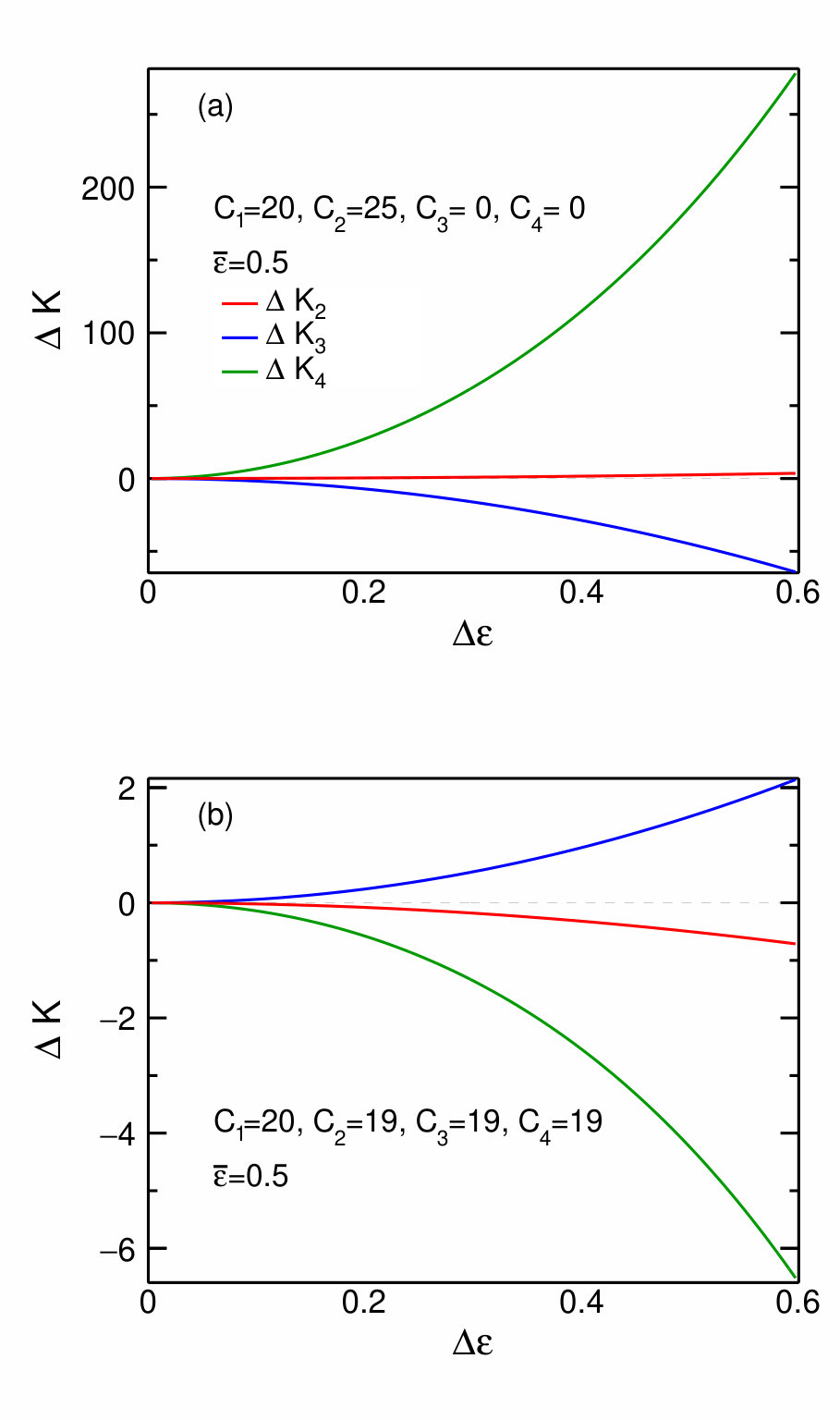 Figure 1
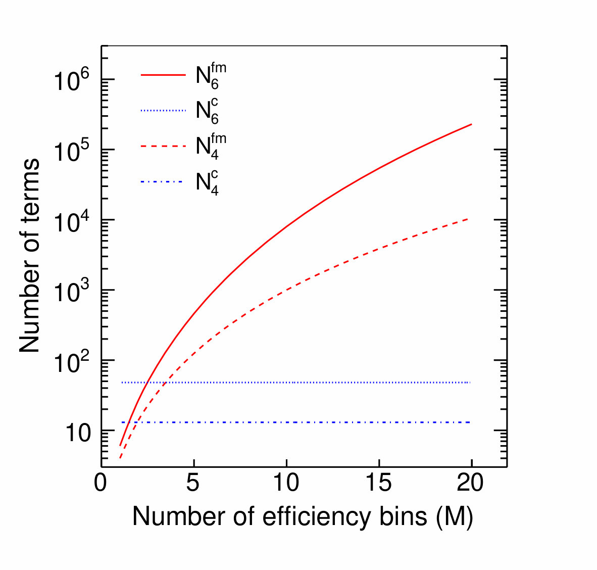 Figure 2
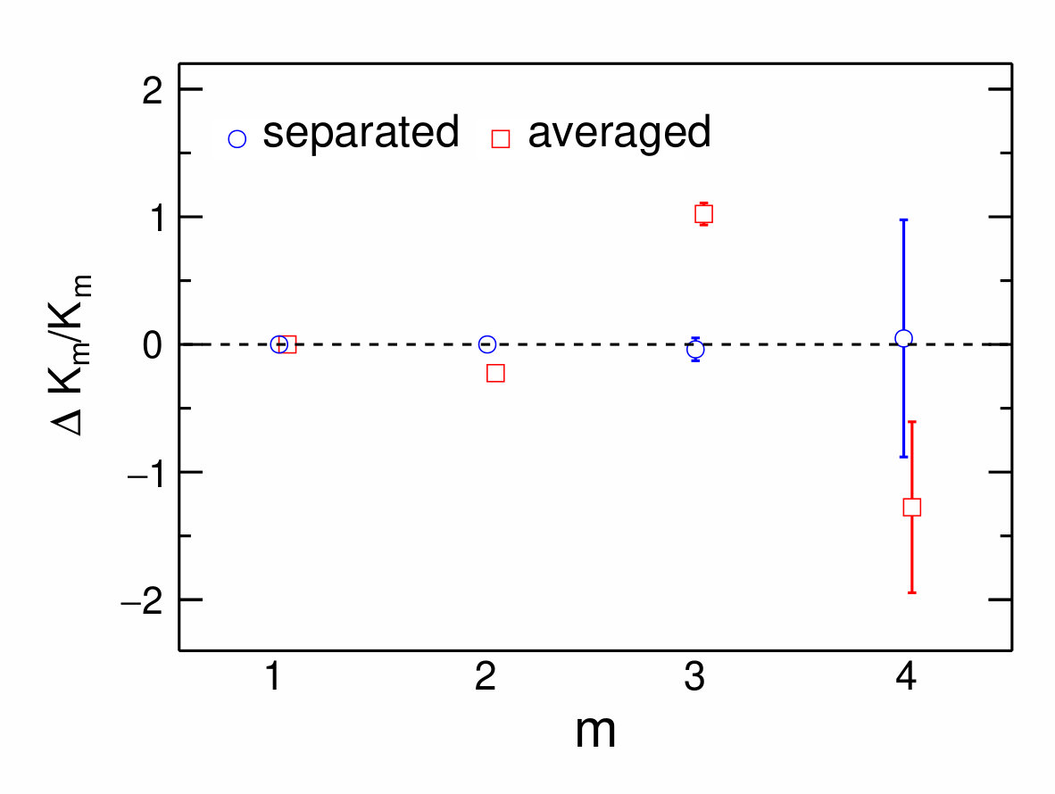 Figure 3
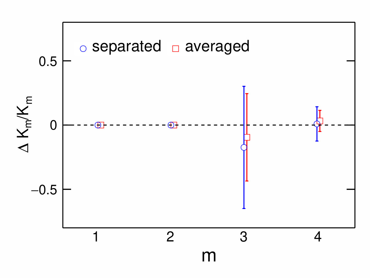 Figure 4
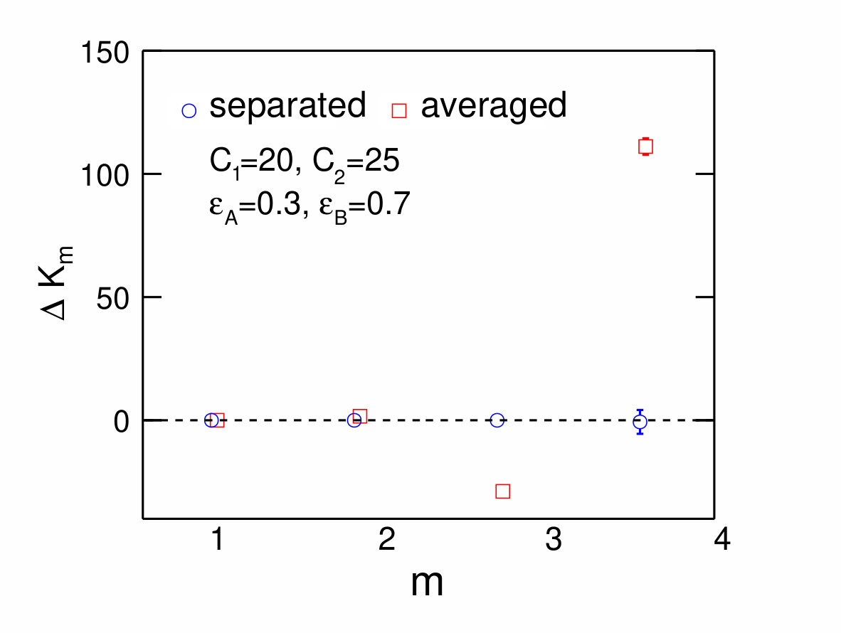 Figure 5
| factorial moment | new method | |
|---|---|---|
| 4 | s | s |
| 8 | s | s |
| 12 | s | s |
| 200 | – | s |
| separated | averaged | analytical | |
|---|---|---|---|
| 1 | |||
| 2 | |||
| 3 | |||
| 4 |
| particles | charge | mean | sigma | efficiency | |
|---|---|---|---|---|---|
| Gauss | 30 | 8 | 0.3 | ||
| Poisson | 10 | – | 0.6 | ||
| Poisson | 8 | – | 0.9 | ||
| Gauss | 25 | 7 | 0.25 | ||
| Poisson | 4 | – | 0.55 | ||
| Poisson | 3 | – | 0.85 |
| charge | mean | sigma | efficiency | |
|---|---|---|---|---|
| Gauss | 20 | |||
| Gauss | 8 |
Peer Reviews
No public reviews on file for this paper yet. If you reviewed it on a platform where reviews are public (OpenReview, ICLR, NeurIPS, ICML), you can paste yours below so the community can read it here.
Videos
No videos yet. Explain this paper in a talk, walkthrough, or lecture? Add one.
More efficient formulas for efficiency correction of cumulants and
effect of using averaged efficiency
Toshihiro Nonaka
Center for Integrated Research in Fundamental Science and Engineering, University of Tsukuba, Tsukuba, Ibaraki 305, Japan
Masakiyo Kitazawa
Department of Physics, Osaka University, Toyonaka, Osaka 560-0043, Japan
J-PARC Branch, KEK Theory Center, Institute of Particle and Nuclear Studies, KEK, 203-1, Shirakata, Tokai, Ibaraki, 319-1106, Japan
ShinIchi Esumi
Center for Integrated Research in Fundamental Science and Engineering, University of Tsukuba, Tsukuba, Ibaraki 305, Japan
Abstract
We derive formulas for the efficiency correction of cumulants with many efficiency bins. The derivation of the formulas is simpler than the previously suggested method, but the numerical cost is drastically reduced from the naïve method. From analytical and numerical analyses in simple toy models, We show that use of the averaged efficiency in the efficiency correction might cause large deviations in some cases and should not be used especially for high order cumulants. These analyses show the importance of carrying out the efficiency correction without taking the average.
pacs:
Valid PACS appear here
††preprint: J-PARC-TH-0084
I Introduction
One of the major goals of heavy ion colliding experiments is to reveal the QCD phase structure. Event-by-event fluctuations of conserved quantities, such as net-baryon and net-charge distributions, have been proposed as experimental probes of the signal from the QCD critical point and phase transitions Asakawa et al. (2000); Jeon and Koch (2000); Ejiri et al. (2006); Stephanov (2009); Asakawa et al. (2009); Friman et al. (2011); see recent reviews Refs. Asakawa and Kitazawa (2016); Luo and Xu (2017). The STAR experiment has measured the beam energy dependencies of the third and fourth order cumulants of net-proton and net-charge multiplicity distributions Adamczyk et al. (2014a, b). In these studies enhancement and suppression of the cumulants at the low energy region are observed, which might be the signal of the critical point. However, there are still large statistical and systematic errors especially at low energy region. The Beam Energy Scan Phase II program is planned at RHIC to accumulate much statistics. In addition, the experimental group is also trying to measure the sixth order cumulant to find the signal of the phase transition Chen (2013).
One of the experimental difficulties in the analyses of higher order cumulants is concerned with finite detector efficiencies. We miss particles with some probability called efficiency, and the imperfect efficiency affects the shape of the event-by-event distributions and their cumulants Kitazawa and Asakawa (2012a); Bzdak and Koch (2012). The correction of this effect has been discussed in the literature Kitazawa and Asakawa (2012a); Bzdak and Koch (2012, 2015); Luo (2015); Kitazawa (2016); Bzdak et al. (2016); Nonaka et al. (2016). Moreover, in real detectors the efficiency often becomes non-uniform for detector acceptance due to many reasons, e.g., detector structures, or detector conditions for certain regions. In this case, the non-uniformity of the efficiency should be taken into account in the correction. Although the efficiency correction with non-uniform efficiencies are proposed in Refs. Bzdak and Koch (2015); Luo (2015); Kitazawa (2016), these methods are difficult to apply to higher order cumulants. In the method proposed in Refs. Bzdak and Koch (2015); Luo (2015), the numerical cost grows proportional to , where is the number of efficiency bins and is the order of the cumulant. Therefore, we cannot increase the numbers of and within a realistic CPU time. In Ref. Kitazawa (2016), other method which drastically reduces the numerical cost has been proposed on the basis of cumulant expansion. In this method, however, the derivation of the analytic formulas becomes complicated for higher order cumulants and it is difficult to apply the method to sixth order. Therefore, an alternative efficient method for this problem is called for.
In the present paper, we propose a new method for the efficiency correction. In this method, the analytic procedure is substantially simplified compared to Ref. Kitazawa (2016). The numerical cost, however, is almost the same as that in Ref. Kitazawa (2016), and drastically smaller than those in Refs. Bzdak and Koch (2015); Luo (2015).
We also apply the formulas to practical problems in experiments. Generally, acceptance uniformity of detectors can be violated due to various practical problems. In this case, it is desirable to divide the efficiency bin into different acceptance regions and apply the efficiency correction with the increased bins. However, it is practically difficult to implement those corrections because of large numerical cost especially for higher order cumulants. Then, one has to use a single averaged efficiency for these acceptance regions. In this paper, we study the effect of using the averaged efficiency in simple toy models. We show that use of the averaged efficiency in the efficiency correction might cause large deviations in some cases and should not be used especially for high order cumulants.
This paper is organized as follows. In Secs. II and III, we derive formulas for the efficiency correction with many efficiency bins. We first derive the result in a simple case with a single efficiency in Sec. II, and then extend it to the multivariate case in Sec. III. In Sec. IV, analytic calculations are performed to study the effect of using averaged efficiency in a toy model. In Sec. V, we study this effect numerically in toy models assuming net-charge fluctuation and non-uniform acceptance.
II Single variable case
Although the main goal of this paper is to derive formulas for the efficiency correction with many efficiency bins, in this section we start from the case with a single efficiency bin, because this analysis serves as a simple illustration of the multivariate case, which will be addressed in the next section.
II.1 Cumulants and factorial cumulants
Let us consider a probability distribution function for an integer stochastic variable . The th order cumulant of is defined as Asakawa and Kitazawa (2016)
[TABLE]
with the cumulant generating function
[TABLE]
In this study, we fully make use of another set of quantities called factorial cumulants , which are defined as
[TABLE]
with the factorial-cumulant generating function
[TABLE]
Cumulants can be represented by the sum of factorial cumulants, and vice versa. To obtain these relations, it is convenient to use the fact that the generating functions (2) and (4) are related with each other by the change of variables, or . The mutual derivatives of and are given by
[TABLE]
Using Eq. (5) the first and second order cumulants are converted into factorial cumulants as
[TABLE]
where it is understood that or is substituted. Repeating the same manipulation, we obtain the relation up to sixth order as
[TABLE]
Using Eq. (6), factorial cumulants can also be expressed in terms of cumulants as
[TABLE]
which are summarized in a compact form
[TABLE]
II.2 Binomial model
Next, we consider the efficiency correction of cumulants in the binomial model Asakawa and Kitazawa (2016). We assume that a multiplicity distribution of a particle number is given by . We then suppose that individual particles are observed with a probability , which is independent for different particles. We denote the number of observed particles as , and the distribution of as . Then, is related to using the binomial distribution function as Asakawa and Kitazawa (2016)
[TABLE]
where the binomial distribution and its factorial-cumulant generating function are given by
[TABLE]
We call Eq. (20) as the binomial model. From Eq. (20), we obtain the factorial-cumulant generating functions of as
[TABLE]
where is the factorial-cumulant generating function of . From Eq. (23), one obtains
[TABLE]
From this result and the definition of the factorial cumulant Eq. (3), we obtain simple relations between the factorial cumulants of and ,
[TABLE]
We note that the same relation holds for factorial moments, which is used in Ref. Bzdak and Koch (2012) to derive the formula of efficiency correction.
II.3 Efficiency correction
In order to perform the efficiency correction, we have to represent in terms of . These relations are obtained by the following three steps:
Convert into using Eqs. (7)–(12). 2. 2.
Convert into using Eq. (25). 3. 3.
Convert into using Eqs. (13)–(18).
The specific procedures for the first and second orders are as follows:
[TABLE]
Similar manipulation up to sixth order are obtained as
[TABLE]
We can extend the manipulation to much higher orders straightforwardly. These relations are equivalent to those given in Ref. Asakawa and Kitazawa (2016), which are obtained based on the cumulant expansion.
III Multivariate case
III.1 Cumulant and factorial cumulant
Next, we extend the analysis in the previous section to the multivariate case. We consider the probability distribution function
[TABLE]
for stochastic variables . Here, with different represent, for example, particle numbers entering detectors which cover different acceptances. We then consider the cumulants of charges, which is given by the linear combination of Kitazawa (2016),
[TABLE]
For example, when one considers the net-baryon number, and for baryons and anti-baryons. For net-electric charge, represents the electric charge of particle .
Defining the cumulant generating function of Eq. (32) as
[TABLE]
the th order cumulant of is given by
[TABLE]
with
[TABLE]
Similarly, the mixed cumulants are defined by
[TABLE]
and so forth. The factorial cumulants of are defined from the generating function Kitazawa and Luo (2017)
[TABLE]
as
[TABLE]
and so forth, with
[TABLE]
The relations between cumulants and factorial cumulants can be obtained similarly to the previous section. Using the fact that and are connected with each other by the change of variables , we obtain
[TABLE]
where we assumed or , and in the last line we defined
[TABLE]
We also define and the symbols with more than two subscripts, such as , in a similar manner. This manipulation can be extended straightforwardly to arbitrary higher orders. In this analysis, we use the following relations between and derivatives valid for :
[TABLE]
Here, represents terms obtained by all possible combinations of subscripts, for example,
[TABLE]
Note that the number shows the total number of the combinations. The conversions from factorial cumulants to cumulants can be carried out with the following relations valid for :
[TABLE]
III.2 Efficiency correction in binomial model
Next, we extend the binomial model Eq. (20) to the multivariate case. We suppose that a particle labeled by is observed with efficiency . Assuming the independence of the efficiencies of individual particles, the probability distribution function of observed particle numbers is related to as Kitazawa (2016)
[TABLE]
The factorial-cumulant generating function of is then given by
[TABLE]
with . From Eq. (56), one finds that and
[TABLE]
and so forth, where it is understood that is substituted and . Equation (57) connects the factorial cumulants of and .
For the efficiency correction, one must represent the cumulants of by those of . Similar to the procedure in Sec. II, these relations are obtained by the following steps:
Convert a cumulant of into factorial cumulants. 2. 2.
Convert the factorial cumulants of into factorial cumulants of . 3. 3.
Convert the factorial cumulants of into cumulants.
The explicit manipulation up to the third order is shown as follows:
[TABLE]
where we defined the linear combination of as
[TABLE]
and so forth. The explicit results up to the sixth order are given by
[TABLE]
where we used
[TABLE]
In Appendix A, we show a specific example of these results for the net-particle number with .
In Eqs. (62)–(III.2), the cumulants of are expressed in terms of the (mixed) cumulants of . These formulas thus can be used for the efficiency correction. We note that the number of cumulants does not depends on the number of efficiency bins . This property is contrasted to the method proposed in Refs. Bzdak and Koch (2015); Luo (2015), in which the number of expectation values to be calculated increases as for th order cumulant. The numerical cost for the efficiency correction with Eqs. (62)–(III.2) thus is drastically reduced compared to the formulas proposed in Refs. Bzdak and Koch (2015); Luo (2015) for large . In the formulas proposed in Ref. Kitazawa (2016), the number of terms is much more reduced compared to Eqs. (62)–(III.2) and thus the numerical cost is smaller than our method. However, the derivation in Ref. Kitazawa (2016) is complicated and it is quite difficult to extend the analysis in Ref. Kitazawa (2016) to sixth and much higher orders. We have numerically verified that our method gives completely the same result as those in Refs. Bzdak and Koch (2015); Luo (2015) and Ref. Kitazawa (2016). In actual analyses, it would be convenient to implement the derivation of Eqs. (62)–(III.2) as a numerical algorithm.
III.3 Mixed cumulants
So far, we considered the efficiency correction of the cumulants of a single charge . Exactly the same discussion can be applied to the efficiency correction of mixed cumulants, which probe correlations between different conserved quantities, e.g, net-baryon, net-strangeness, and net-charge. Below we show the formulas for mixed cumulants \bigl{<}Q_{(x)}^{m_{1}}Q_{(y)}^{m_{2}}\bigr{>} up to fourth order ():
[TABLE]
where we used the symbol
[TABLE]
III.4 Calculation cost
Finally we discuss how efficient Eqs. (62)–(III.2) are compared to the conventional method based on factorial moments Bzdak and Koch (2015). In the conventional method, a cumulant is decomposed into mixed factorial moments. In this decomposition for an th order cumulant, all possible combinations of mixed factorial moments between different efficiency bins with order satisfying appear. The number of the th order factorial moments is given by with being different efficiency bins. The total number of the mixed factorial moments satisfying is thus given by
[TABLE]
When this method is adopted to the analysis of the net-particle number, the numbers of efficiency bins of particle and anti-particle are given by .
Assuming that the numerical cost to calculate one mixed factorial moment is insensitive to the order, the cost in the conventional method is proportional to Eq. (74), which grows as for large . On the other hand, in the new method with Eqs. (62)–(III.2), the total number of cumulants,
[TABLE]
is independent of . By comparing Eqs. (74) and (75), it is clear that the new method becomes more advantageous for larger especially for higher order cumulants. In the actual numerical analyses, the cost to calculate one factorial moment or cumulant can grow with increasing depending on the implementation and data structure. As this dependence can be common for both methods, we neglect this effect here. In Fig. 1 we show the number of terms in both methods, Eqs. (74) and (75), as functions of for fourth and sixth orders.
In Table 1, we show the comparison of the CPU time to calculate the sixth order cumulant in both methods in specific implementations. The codes are executed on the same CPU (3GHz Intel Core i7) for events and , , , and . One finds that the CPU time with the conventional method rapidly increases as becomes larger, while CPU time in the new method is insensitive to ; even with , the CPU time is only about twice larger than in the new method. This result is consistent with the cost estimate in Fig. 1. Moreover, the new method is about two order faster than the conventional one already at . We, however, note that the calculation cost, of coarse, is strongly dependent on the implementation.
It is also notable that the new method is advantageous in simplifying the code and reducing momory resource.
IV Two-distribution model
In the rest of this paper we focus on the effect of using the averaged efficiency for different efficiency bins. In this section, we first consider a simple problem which can be treated analytically.
We consider a measurement of two kinds of particle number distributions and by detectors having different efficiencies and , respectively. We assume that the two distributions are equivalent and independent, and their cumulants are given by
[TABLE]
We are interested in the cumulants of the total particle number . Due to the additive property of cumulants for independent stochastic variables Asakawa and Kitazawa (2016), cumulants of are given by
[TABLE]
Because of the efficiency loss, the observed particle numbers and have different distributions from those of and . The cumulants of and are represented by by the inverse procedure of Eqs. (26) and (27) Asakawa and Kitazawa (2016). For the first and second orders we have
[TABLE]
with A and B. By substituting Eqs. (78) and (79) into Eqs. (62) and (63) with , the correct value of is recovered.
Now, we consider a case that the efficiency correction is performed by regarding as a particle number described by a single distribution function measured by an averaged efficiency . Then, the efficiency correction would be performed by substituting and into the result in Sec. II such as Eqs. (26) and (27). For the first order, the result of this efficiency correction is
[TABLE]
Therefore, the correct cumulant Eq. (77) is recovered to this order. This, however, is not the case for higher order cumulants. By denoting the deviation of the reconstructed cumulant with average efficiency from the original one as
[TABLE]
is calculated to be
[TABLE]
with . The nonzero shows that the reconstructed cumulant does not agree with the original one. These results clearly show that the use of the averaged efficiency gives rise to a deviation in the result of the efficiency correction. Only for Poisson distribution (), the deviation vanishes.
Let us see in specific distributions. We first consider a Gauss distributions with and for . In the top panel of Fig. 2, with are plotted as functions of . One finds that becomes large with increasing and . Next, we consider a distribution with and for ; this distribution is close to Poissonian but cumulants higher than the first order are 5% smaller than Poissonian values. The dependencies of in this case is shown in the bottom panel of Fig. 2. From the figure, one again obtains the same conclusion that becomes large for higher orders and larger . These results show the importance of the use of the separated efficiencies in the experimental analysis especially for higher orders.
V Numerical analysis in toy models
In this section, we study the effects of using averaged efficiency numerically in toy models by generating random events.
V.1 Two-distribution model
First, we analyze the two-distribution problem discussed in the previous section numerically. Two particle numbers and are independently generated according to Gauss distribution, and they are randomly sampled with the efficiencies and to obtain the measured particle numbers and . We generated 100M events, and this analysis was repeated 30 times independently for the estimate of the statistical error. We perform the efficiency correction by the following two methods:
Efficiency correction with separated efficiencies for A and B. 2. 2.
Efficiency correction using the averaged efficiency .
We set , , , and .
The results of in these analyses are shown in Fig. 3 as a function of the order of the cumulant . Blue circles are the results with separated efficiency correction. The figure shows that they reproduce correct input cumulants with within statistical error. Red squares represent results from the averaged efficiency. The figure shows that these results give wrong values with for . These deviations are compared with the analytic results in Eqs. (82)–(84) in Tab. 2. The table shows that they are consistent with each other.
V.2 Averaged efficiencies for different particle species
In IV and V.1, we discussed the case with a single particle species with a unit charge. Next we extend the discussion to the case of the net-charge fluctuation. In this case, we measure the charged particles without particle identifications, and there seems to be no problem to use averaged efficiency of charged particles for the correction. However, when we consider the fact that the charged particles mainly consist of , and , this assumption would be violated, because those particles have different efficiencies experimentally and their net-particle distributions could have different probability distributions. Therefore, we perform a toy model analysis in order to study the effect of using the averaged efficiency assuming the net-charge distribution. At high beam energies, one can expect that produced pions distribution is closer to the Gaussian than kaons and protons due to the large production of pions. In this toy model, therefore, we simply set the distribution for as Gauss distribution as an extreme case, while for and as Poisson distributions. These particles are observed with different efficiencies for different particle species. These different efficiencies are used in the analysis of separated efficiency correction. We also perform the efficiency correction with the averaged efficiencies for positively and negatively charged particles
[TABLE]
where denotes particle species (, , ) and is number of produced particles. Note that the use of the averaged efficiency for positively and negatively charged particles derives other artificial effects discussed in Ref. Nonaka et al. (2016). Parameters are shown in Tab. 3.
Relative deviation of efficiency corrected th order cumulant from input value are shown in Fig. 4 up to the fourth order. The figure shows that the result with the averaged efficiencies again cannot reproduce the correct value. Thus, we must not use averaged efficiency if there are different physics in different efficiency bins.
V.3 Two detectors with a common source
In current analysis for net-proton distribution at STAR, efficiency bin is divided into two regions, and GeV/c eff (2015), because the measurement of particles are performed in different ways for these regions: Energy loss measured by Time Projection Chamber (TPC) is used for proton identification at GeV/c, while the mass squared measured by Time Of Flight (TOF) detector is also used at GeV/c. By including TOF detector, the efficiency drops at GeV/c. This dependent efficiency is implemented by dividing region at GeV/c. Similarly, efficiencies would depend on direction. TPC and TOF cover full azimuthal angle and have excellent particle identification capability. However, some of the TPC sectors are sometimes in a bad condition, which leads to the nonuniform acceptance in the direction. Let us discuss the effect by using the averaged efficiency in these conditions assuming two detectors, which may not be the case discussed in V.2, because the distribution at each detector would not be determined separately. In other words, even if there are different kinds of particle distributions, we cannot identify those distributions at the detector level.
Setup for the toy model is as follows. Particles are randomly generated according to Gauss distributions , and let those particles randomly incident on the detector A or B with 50% probability. Then particles are randomly sampled by efficiencies and . We apply efficiency correction on and with separated efficiencies or with averaged efficiency between two detectors. We consider the net particle number by generating charge particles assuming the measurement of net-proton number cumulants. Parameters are shown in Tab. 4.
The last row in Tab. 4 represents efficiencies that are characterized for each detector and electric charge. Results of are shown in Fig. 5. From the figure, one finds that there is no deviation for all the order of cumulants. Note that the value of the denominator is not common for different . This leads to the larger error for third order than fourth order in Fig. 5. At first glance this looks strange, but we can provide a simple explanation as follows. When one focuses on a particle in this model, it is measured with a probability randomly and independently. Therefore, this is exactly the case of single efficiency bin with the averaged efficiency. This result indicates that the efficiency correction with averaged efficiency works well when underlying physics is identical for different efficiency bins. However, for nonuniform acceptance in real experiment, one needs to check whether the results obtained from averaged efficiencies are consistent with the separated efficiencies.
VI Summary
In this paper, we derived formulas for the efficiency correction with many efficiency bins. In our method, the formulas are obtained easily compared to Ref. Kitazawa (2016), but the numerical cost is drastically reduced compared to Refs. Bzdak and Koch (2015); Luo (2015) when the number of efficiency bins and order of the cumulant are large. The efficiency correction for higher order cumulants with many bins thus can be carried out effectively in our method. The result is then applied to the efficiency correction in simple models to study the effect of using averaged efficiency in Secs. IV and V. We have shown that the use of the averaged efficiency can lead to wrong corrected values if underlying physics is different in efficiency bins. This result indicates that separated efficiencies have to be used to perform the efficiency correction correctly. For example, it would be important to take account of the nonuniform acceptance along azimuthal angle and the dependencies of efficiency for the accurate efficiency correction.
Final remarks are in order. First, although we used the binomial model throughout this paper, this model is justified only when the efficiencies for individual particles are independent Asakawa and Kitazawa (2016). When the correlations between individual particles are not negligible, these effects have to be considered Bzdak et al. (2016). Second, experimental analyses usually measure proton number cumulants as proxies of baryon number cumulants. In Refs. Kitazawa and Asakawa (2012b, a), it is shown that the measurement of protons corresponds to the measurement of baryons with efficiency loss. Therefore, the baryon number cumulants can in principle be constructed from those of protons using efficiency correction. In this case, the use of the binomial model is justified owing to isospin randomization Kitazawa and Asakawa (2012b).
VII Acknowledgement
The authors thank X. Luo and N. Xu for useful discussions. T. N. thanks P. Tribedy for the idea of the toy model discussed in Sec. V.2. M. K. thanks stimulating discussions in the INT program “Exploring the QCD Phase Diagram through Energy Scans”, Seattle, Sep. 19 – Oct. 14, especially A. Bzdak and V. Koch. We acknowledge support from MEXT and JSPS KAKENHI Grant Number 25105504 and Super Global University Program in University of Tsukuba.
Appendix A Net-particle in simple case
In the case of net-particle with single efficiency bin, explicit formulas for efficiency correction can be derived from Eqs. (62)–(68) by substituting , , , and . By defining and , the formulas up to sixth order are given by
[TABLE]
The reference list from the paper itself. Each links out to its DOI / PubMed record.
- 1Asakawa et al. (2000) M. Asakawa, U. W. Heinz, and B. Muller, Phys. Rev. Lett. 85 , 2072 (2000) , ar Xiv:hep-ph/0003169 [hep-ph] . · doi ↗
- 2Jeon and Koch (2000) S. Jeon and V. Koch, Phys. Rev. Lett. 85 , 2076 (2000) , ar Xiv:hep-ph/0003168 [hep-ph] . · doi ↗
- 3Ejiri et al. (2006) S. Ejiri, F. Karsch, and K. Redlich, Phys. Lett. B 633 , 275 (2006) , ar Xiv:hep-ph/0509051 [hep-ph] . · doi ↗
- 4Stephanov (2009) M. A. Stephanov, Phys. Rev. Lett. 102 , 032301 (2009) , ar Xiv:0809.3450 [hep-ph] . · doi ↗
- 5Asakawa et al. (2009) M. Asakawa, S. Ejiri, and M. Kitazawa, Phys. Rev. Lett. 103 , 262301 (2009) , ar Xiv:0904.2089 [nucl-th] . · doi ↗
- 6Friman et al. (2011) B. Friman, F. Karsch, K. Redlich, and V. Skokov, Eur. Phys. J. C 71 , 1694 (2011) , ar Xiv:1103.3511 [hep-ph] . · doi ↗
- 7Asakawa and Kitazawa (2016) M. Asakawa and M. Kitazawa, Prog. Part. Nucl. Phys. 90 , 299 (2016) , ar Xiv:1512.05038 [nucl-th] . · doi ↗
- 8Luo and Xu (2017) X. Luo and N. Xu, (2017), ar Xiv:1701.02105 [nucl-ex] .