Coupling of multiscale and multi-continuum approaches
Eric T. Chung, Yalchin Efendiev, Tat Leung, Maria Vasilyeva

TL;DR
This paper explores the relationship between multi-continuum methods and the Generalized Multiscale Finite Element Method (GMsFEM), proposing a coupled approach for efficient simulation of fractured media with multiscale features.
Contribution
It establishes a connection between multi-continuum techniques and GMsFEM, and introduces a coupled multiscale modeling approach for complex fractured media.
Findings
GMsFEM can automatically identify fracture networks.
Simplified basis construction is effective for known, simple fracture geometries.
Coupled approach efficiently models unresolved fractures using multi-continuum methods.
Abstract
Simulating complex processes in fractured media requires some type of model reduction. Well-known approaches include multi-continuum techniques, which have been commonly used in approximating subgrid effects for flow and transport in fractured media. Our goal in this paper is to (1) show a relation between multi-continuum approaches and Generalized Multiscale Finite Element Method (GMsFEM) and (2) to discuss coupling these approaches for solving problems in complex multiscale fractured media. The GMsFEM, a systematic approach, constructs multiscale basis functions via local spectral decomposition in pre-computed snapshot spaces. We show that GMsFEM can automatically identify separate fracture networks via local spectral problems. We discuss the relation between these basis functions and continuums in multi-continuum methods. The GMsFEM can automatically detect each continuum and…
Click any figure to enlarge with its caption.
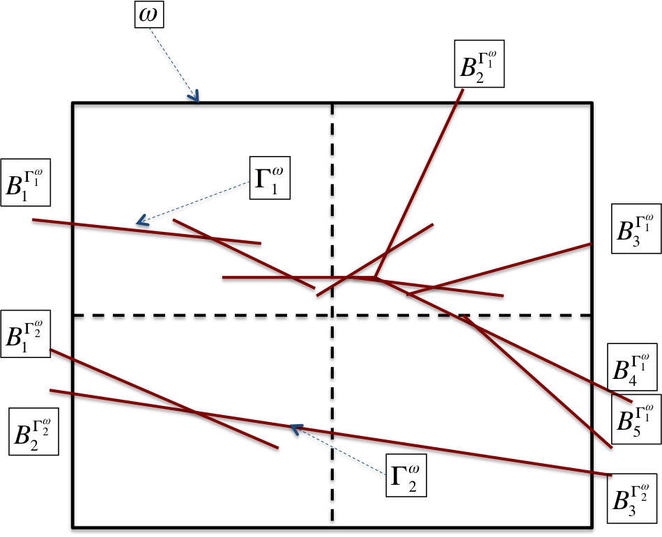 Figure 1
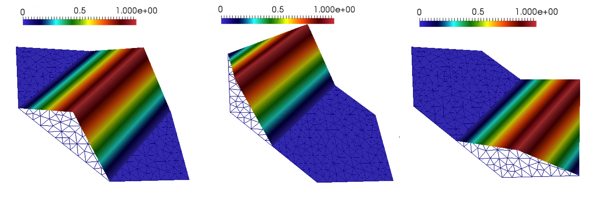 Figure 2
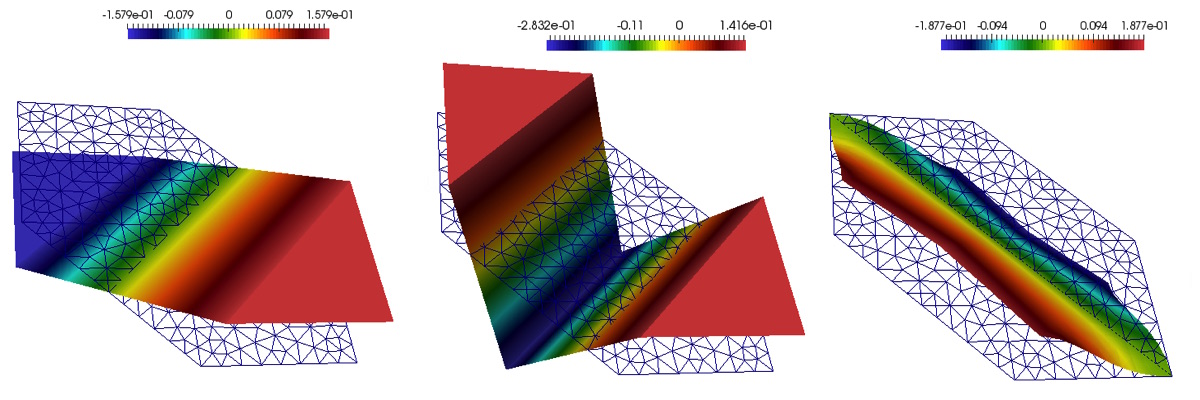 Figure 3
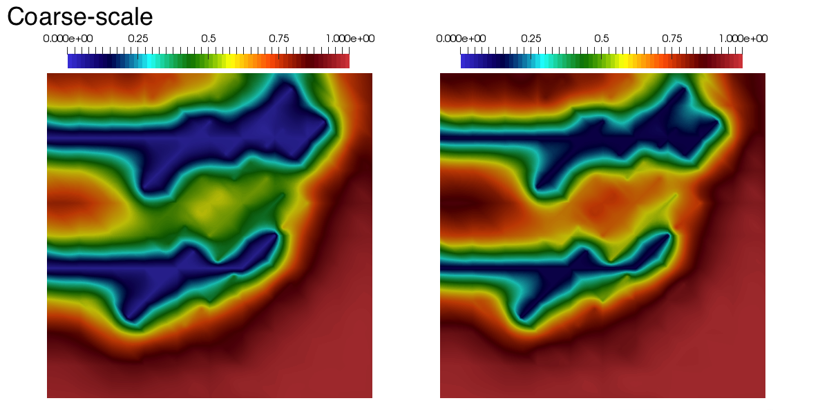 Figure 4
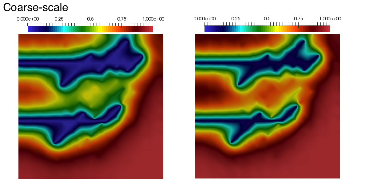 Figure 5
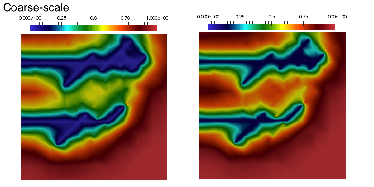 Figure 6
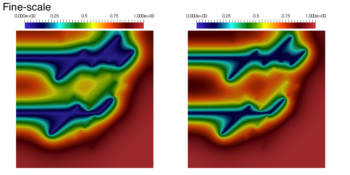 Figure 7
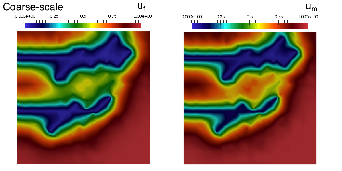 Figure 8
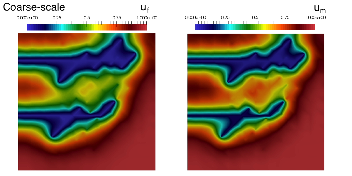 Figure 9
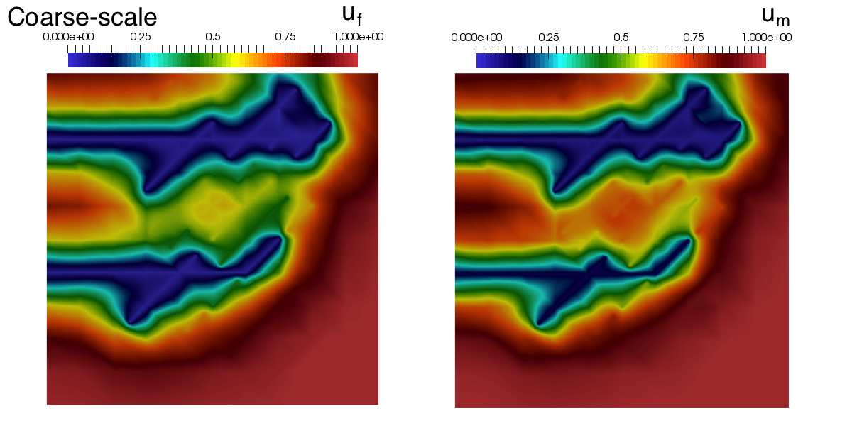 Figure 10
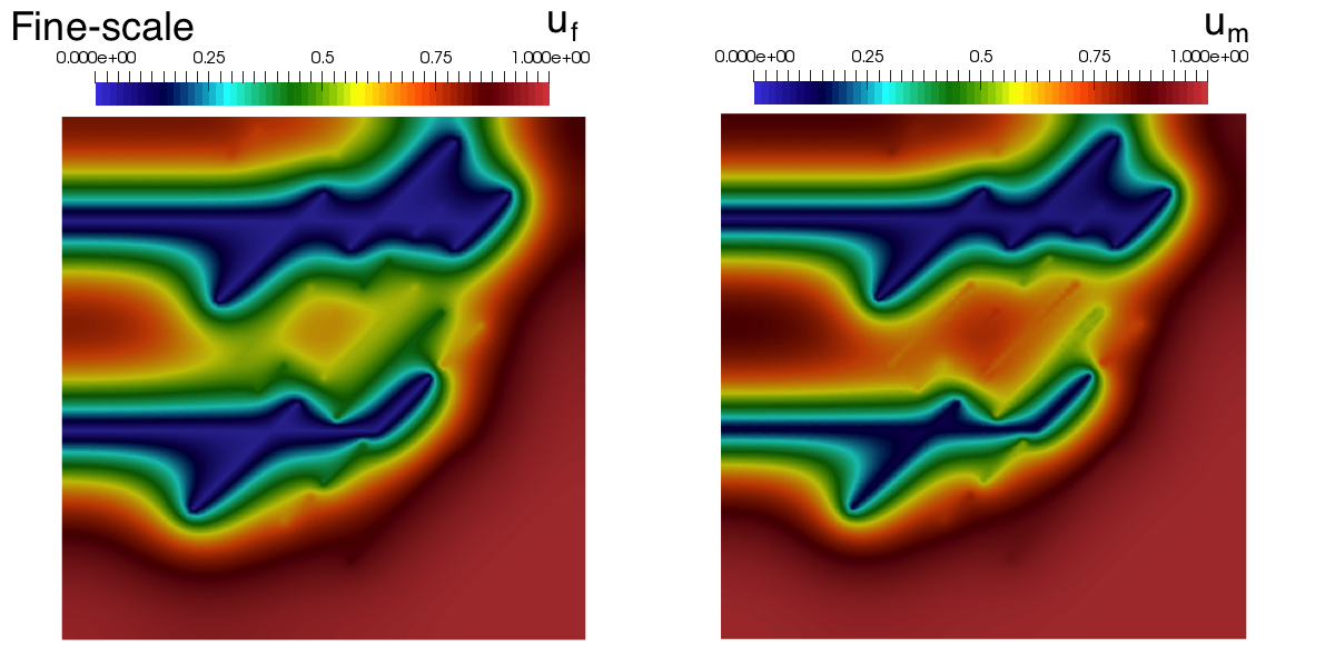 Figure 11
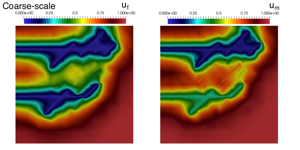 Figure 12
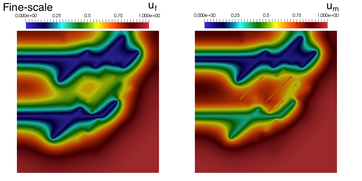 Figure 13
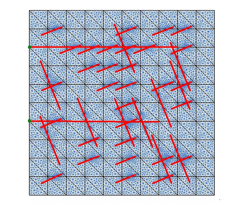 Figure 14
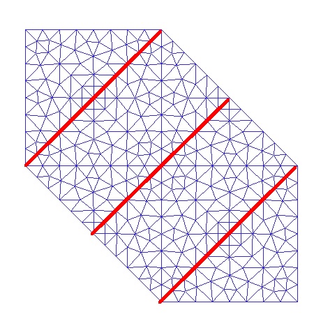 Figure 15
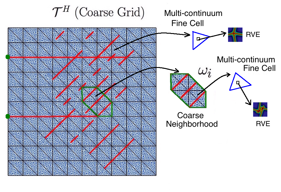 Figure 16
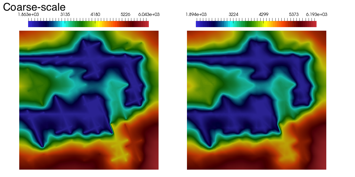 Figure 17
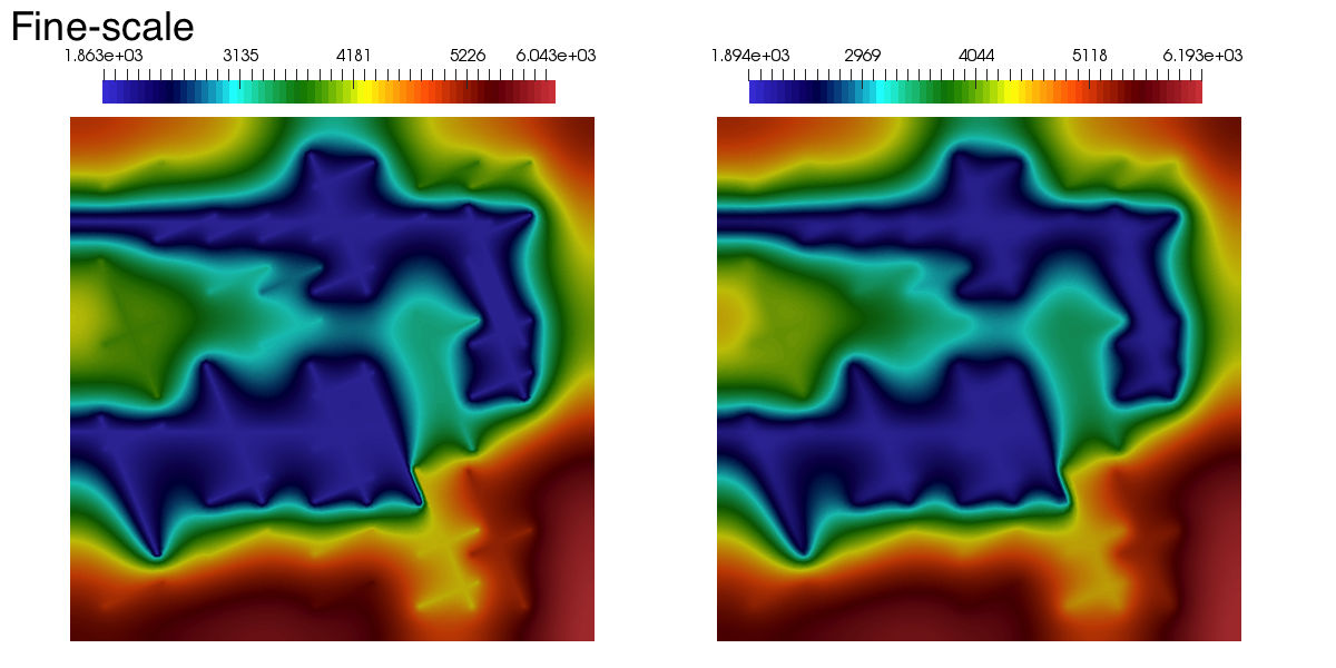 Figure 18
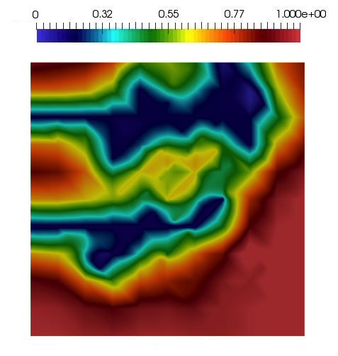 Figure 19
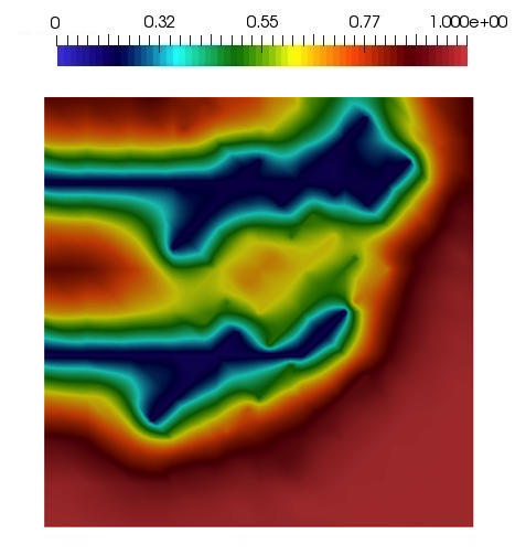 Figure 20
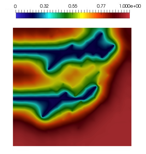 Figure 21
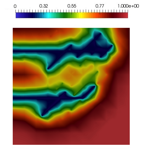 Figure 22
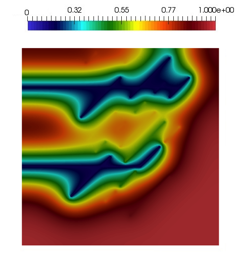 Figure 23
| dim() | |||
|---|---|---|---|
| Standard GMsFEM | |||
| 1 | 121 | 49.067 | 79.885 |
| 2 | 242 | 9.116 | 36.499 |
| 3 | 363 | 2.325 | 8.099 |
| 4 | 484 | 1.413 | 3.919 |
| 5 | 605 | 0.883 | 2.658 |
| 6 | 726 | 0.708 | 1.795 |
| 8 | 968 | 0.253 | 0.348 |
| 16 | 1936 | 0.095 | 0.089 |
| GMsFEM by | |||
| 184 | 13.554 | 45.342 | |
| 275 | 2.651 | 11.377 | |
| 396 | 1.582 | 4.414 | |
| Simplified basis functions | |||
| all | 268 | 1.850 | 3.799 |
| dim() | ||||||
|---|---|---|---|---|---|---|
| Standard GMsFEM (un-coupled) | ||||||
| 6 | 1452 | 0.846 | 1.966 | 0.846 | 15.938 | 4.519 |
| 8 | 1936 | 0.297 | 0.379 | 0.297 | 15.835 | 4.093 |
| 12 | 2904 | 0.148 | 0.188 | 0.148 | 14.213 | 3.670 |
| 16 | 3872 | 0.106 | 0.087 | 0.106 | 11.769 | 3.041 |
| Simplified basis functions (un-coupled) | ||||||
| all | 536 | 2.386 | 3.831 | 2.386 | 21.765 | 6.713 |
| Standard GMsFEM (coupled) | ||||||
| 6 | 1452 | 1.919 | 2.767 | 1.919 | 9.919 | 3.588 |
| 8 | 1936 | 1.052 | 1.154 | 1.052 | 2.840 | 1.335 |
| 12 | 2904 | 0.354 | 0.550 | 0.354 | 1.325 | 0.628 |
| 16 | 3872 | 0.124 | 0.102 | 0.124 | 0.643 | 0.194 |
| Simplified basis functions (coupled) | ||||||
| all | 830 | 2.056 | 3.439 | 2.056 | 6.234 | 3.690 |
| dim() | ||||||
|---|---|---|---|---|---|---|
| Standard GmsFEM (un-coupled) | ||||||
| 6 | 1452 | 0.837 | 1.925 | 0.837 | 30.542 | 13.869 |
| 8 | 1936 | 0.293 | 0.358 | 0.293 | 26.427 | 11.912 |
| 12 | 2904 | 0.148 | 0.193 | 0.148 | 23.165 | 10.440 |
| 16 | 3872 | 0.108 | 0.089 | 0.108 | 17.945 | 8.086 |
| Simplified basis functions (un-coupled) | ||||||
| all | 536 | 2.343 | 3.870 | 2.343 | 36.649 | 16.872 |
| Standard GmsFEM (coupled) | ||||||
| 6 | 1452 | 1.944 | 2.584 | 1.944 | 6.942 | 3.934 |
| 8 | 1936 | 1.070 | 1.200 | 1.070 | 2.197 | 1.452 |
| 12 | 2904 | 0.359 | 0.544 | 0.359 | 0.788 | 0.606 |
| 16 | 3872 | 0.129 | 0.105 | 0.129 | 0.375 | 0.193 |
| Simplified basis functions (coupled) | ||||||
| all | 830 | 2.105 | 3.399 | 2.105 | 4.122 | 3.557 |
Peer Reviews
No public reviews on file for this paper yet. If you reviewed it on a platform where reviews are public (OpenReview, ICLR, NeurIPS, ICML), you can paste yours below so the community can read it here.
Videos
No videos yet. Explain this paper in a talk, walkthrough, or lecture? Add one.
Taxonomy
TopicsAdvanced Mathematical Modeling in Engineering · Advanced Numerical Methods in Computational Mathematics · Enhanced Oil Recovery Techniques
Coupling of multiscale and multi-continuum approaches
Eric T. Chung Department of Mathematics, The Chinese University of Hong Kong (CUHK), Hong Kong SAR. Email: [email protected]. The research of Eric Chung is supported by Hong Kong RGC General Research Fund (Project 400411).
Yalchin Efendiev Department of Mathematics & Institute for Scientific Computation (ISC), Texas A&M University, College Station, Texas, USA. Email: [email protected].
Tat Leung Department of Mathematics, Texas A&M University, College Station, TX 77843
Maria Vasilyeva Department of Computational Technologies, Institute of Mathematics and Informatics, North-Eastern Federal University, Yakutsk, Republic of Sakha (Yakutia), Russia, 677980 & Institute for Scientific Computation, Texas A&M University, College Station, TX 77843-3368
Abstract
Simulating complex processes in fractured media requires some type of model reduction. Well-known approaches include multi-continuum techniques, which have been commonly used in approximating subgrid effects for flow and transport in fractured media. Our goal in this paper is to (1) show a relation between multi-continuum approaches and Generalized Multiscale Finite Element Method (GMsFEM) and (2) to discuss coupling these approaches for solving problems in complex multiscale fractured media. The GMsFEM, a systematic approach, constructs multiscale basis functions via local spectral decomposition in pre-computed snapshot spaces. We show that GMsFEM can automatically identify separate fracture networks via local spectral problems. We discuss the relation between these basis functions and continuums in multi-continuum methods. The GMsFEM can automatically detect each continuum and represent the interaction between the continuum and its surrounding (matrix). For problems with simplified fracture networks, we propose a simplified basis construction with the GMsFEM. This simplified approach is effective when the fracture networks are known and have simplified geometries. We show that this approach can achieve a similar result compared to the results using the GMsFEM with spectral basis functions. Further, we discuss the coupling between the GMsFEM and multi-continuum approaches. In this case, many fractures are resolved while for unresolved fractures, we use a multi-continuum approach with local Representative Volume Element (RVE) information. As a result, the method deals with a system of equations on a coarse grid, where each equation represents one of the continua on the fine grid. We present various basis construction mechanisms and numerical results. The GMsFEM framework, in addition, can provide adaptive and online basis functions to improve the accuracy of coarse-grid simulations. These are discussed in the paper. In addition, we present an example of the application of our approach to shale gas transport in fractured media.
1 Introduction
Multiscale phenomena in fractured media. Subsurface formations with discrete fractures, faults, thin features are common in many applications. These include fractured subsurface formations, fractured composite materials, and so on. A main challenge in simulating complex processes is due to multiple scale and high contrast. The material properties within fractures can be very different from the background properties. Due to complex fracture configurations, there are multiple scales and high contrast.
Fine-grid simulation for fractures. Constructing a fine-grid simulation model is typically done in several steps (we refer [21] for the overview). As a first step, an unstructured grid is used to describe the fractures. Then, the flow/transport equations are discretized on the unstructured grid. A variety of techniques have been applied for flow simulation in porous media with discrete fractures using both finite-element and finite-volume methods. Within the finite-element framework, the standard Galerkin formulation ([5, 20, 23, 25]), the mixed finite-element method ([15, 19, 26, 27]), and the discontinuous Galerkin method ([14, 18]) have been used to simulate single-phase and multiphase flow in discrete fracture models. Within the finite-volume framework, formulations have been presented by, e.g., [7, 17, 22, 29, 31, 33]. A hybrid approach combining the finite-element method for the pressure equation and the finite volume method for transport has also been investigated ([16, 28, 30]).
The need for model reduction. Because of multiple scales and high contrast, some type of model reduction is needed for simulating physical processes in fractured media. Typical approaches divide the domain into coarse grids, where effective properties in each coarse-grid block are computed [11, 35]. The standard upscaling methods compute the effective properties using the solution of local problems in each coarse block or representative volume. However, it is known that these approaches are not sufficient as each coarse block contains multiple important modes. This led to multi-continuum approaches [4, 6, 24, 32, 34, 36], where several equations are formulated for each coarse block. In particular, the flow equation for the background (called matrix) and the fracture are written separately with some interaction terms. These approaches make several assumptions such as each continua connected throughout the domain and the form of the coupling. Our goal is to show a relation between these approaches and some multiscale finite element methods and further discuss generalizations based on these approaches.
Brief introduction to the GMsFEM. The GMsFEM [9, 10, 12] follows the framework of the Multiscale Finite Element Method (MsFEM) and is introduced to systematically add new degrees of freedom in each coarse block. The new basis functions are computed by constructing the snapshots and performing local spectral decomposition in the snapshot space. It was shown that there is a spectral gap and the eigenvectors corresponding to very small eigenvalues represent the connected high-conductivity networks. These dominant eigenvectors represent fracture networks and can be thought as reduced degrees of freedom representing each continua as explained later.
**This paper. ** In this paper, we discuss a relation between the GMsFEM and the multi-continuum approaches. As mentioned, the dominant eigenvectors represent the connected fracture networks. For example, if there are separate fracture networks within a coarse block, then we will have very small eigenvalues and the corresponding eigenvectors represent these fracture networks. We give a detailed comparison between the multi-continua approaches and the GMsFEM in the paper. We discuss the interaction between different continuum media. In multi-continuum approaches, this interaction is modeled based on physical principles, while the GMsFEM approach provides a rigorous coupling between multiple continua. We note the GMsFEM automatically takes into account the interaction of various continua between different coarse blocks, while in multi-continuum approaches, this interaction is stated apriori based on physical principles [37]. We also present simplified basis functions that are related to fractures if the fracture networks are identified.
In the paper, we discuss a coupled GMsFEM and the multi-continuum approaches by considering fractures over a very rich hierarchy of scales. Our approach uses multi-continuum at the fine grid and the GMsFEM for modeling the fractures that can be resolved on the fine grid (see Figure 1). In this case, the method deals with a system of equations coupled with the fracture network. First, we discuss a GMsFEM for this system. Secondly, we discuss approaches for computing the parameters of the multi-continuum system based on local Representative Volume Element (RVE) computations. We discuss the setup of local RVE problems and compute the parameters for the multi-continuum fine-grid discretization. Since these parameters, in general, are heterogeneous, the use of coupled basis functions is crucial, and their constructions will be presented. We will also discuss a relation between the GMsFEM and the Multiple Interacting Continua (MINC) [32].
On the other hand, we establish a relation between offline GMsFEM and the multi-continua approaches. The GMsFEM has several important fundamental ingredients that can further be used to achieve higher accuracy and more efficiency. The first ingredient includes the adaptivity. The GMsFEM’s adaptivity can be used to add multiscale basis functions in selected regions. This concept can be effectively used to add new multiscale basis functions in selected regions. The second ingredient of the GMsFEM is online basis functions. These basis functions are constructed using the residual information (adaptively in space and time) to speed-up the simulations. This can be used to speed-up the convergence of the proposed method.
We will show numerical results. First, we discuss the GMsFEM’s basis construction and numerically show how to identify the number of continua based on local spectral decomposition and the spectrum. Then, we present a simplified basis construction and numerical results for the GMsFEM using both simplified basis construction and a general approach. In the second part, we demonstrate numerical results when the GMsFEM and the multi-continuum approaches are coupled. In this case, the multi-continuum approach is used on the fine grid. Our numerical results use both coupled and un-coupled basis functions and show that the GMsFEM is able to couple with the multi-continuum appraoch and gives accurate solution using few basis functions. The GMsFEM can be used for heterogeneously varying multi-continuum problems. In [2], we have applied the GMsFEM to shale gas flows in multi-continuum media. In this paper, we also present an example of the application of our proposed approach to shale gas transport.
Furthermore, we will present an analysis for the GMsFEM when the fine-scale problem is described by a multi-continuum approach. In this case, the method gives a system of coupled equations. We study the convergence of the GMsFEM for cases when basis functions are independently constructed and in a coupled fashion. In both cases, convergence results are obtained.
The paper is organized as follows. In Section 2, we discuss the relation between the GMsFEM and multi-continuum approaches. We develop simplified basis functions and show numerical results. In Section 3, we discuss the coupled GMsFEM and the multi-continuum approach. We also show numerical results in this section. The analysis is given in the Appendix A.
2 Relation between the GMsFEM and multi-continuum
The goal of this section is to highlight the similarities between the multi-continuum approaches and the GMsFEM. We assume that the fractures are resolved on a fine grid. We show that (1) the GMsFEM can identify fracture networks and result in a similar system as a multi-continuum approach, (2) the GMsFEM can resolve the detailed fracture and matrix interaction, and (3) the GMsFEM basis functions can be computed in a simplified way.
2.1 Fine-grid equations in fractured media
We consider a detailed fine-grid discretization of the flow equation in the fractured media
[TABLE]
where is the solution, is the source term, is permeability and is porosity. The permeability is large within fractures and the porosity has a smaller value in the fractures. Fractures are modeled as one dimensional objects.
The domain is divided into the fracture and the matrix region
[TABLE]
where and represent the matrix and the fracture regions. denotes the aperture of the -th fracture and is the index of the fractures. We denote by the permeability of the -th fracture. is a two-dimensional domain and is a one-dimensional domain. The system is written in a finite-element discretization. We introduce the concepts of fine and coarse grids. Let be a coarse-grid partition (computational grid) of the computational domain into finite elements (triangles, quadrilaterals, tetrahedra, etc.). We assume that each coarse element is partitioned into a connected union of fine grid blocks. The fine-grid partition will be denoted by , and is by definition a refinement of the coarse grid . We use (where denotes the number of coarse nodes) to denote the vertices of the coarse mesh and define the neighborhood of the node by
[TABLE]
See Figure 1 for illustration.
The bilinear form for the resulting system is
[TABLE]
where is the fine-grid finite element function, is the derivative along the fracture lines, and porosity and permeability in the matrix, and porosity and permeability in the fractures, and . The fracture permeability and porosity include the aperature information . We remind that in our setup, we assume that a fine grid resolves some set of fractures (very detailed), while each fine grid can contain many small fractures (see Figure 1), i.e., multi-continua.
2.2 Multi-continuum approach. A brief summary.
The multi-continuum approach is an average model, which is solved on a coarse grid. We denote the solution for -th continuum by and assume that each continuum interacts with every other, for the sake of generality. Then, we can write the resulting system as
[TABLE]
where is an exchange term, which can contain both space and time derivates of ’s [4, 6, 24, 32, 34, 36]. In a special case when each continuum only interacts with the background, if the background is , then
[TABLE]
where is the source term. We write this equation as
[TABLE]
where is solved on a coarse grid using standard basis functions and is a standard basis function.
2.3 A brief overview of the GMsFEM.
We discuss the use of the GMsFEM on a coarse grid. The GMsFEM uses the coarse grid and constructs a local reduced-order model for each coarse block, by constructing snapshot solutions and extracting basis functions. Snapshots are constructed by solving local problems subject to some boundary conditions. Below, we briefly discuss the snapshot calculations and the basis computations.
2.3.1 Snapshots and multiscale basis.
We briefly describe the construction of the snapshot space . We refer to [9, 12] for further discussions. The snapshot space consists of local solutions. Harmonic functions can be used to construct a snapshot space. We define , where , where denotes the fine-grid boundary node on and solve the local problems with as boundary conditions. More precisely, given a fine-scale piecewise linear function defined on ( is a coarse block and we omit the index ), we define by the following variational problem
[TABLE]
and on . Note that the source is also placed on fracture boundaries. The snapshot space is defined as
[TABLE]
where is the number of functions in the snapshot space in (a generic coarse block). We also denote
[TABLE]
We note that the randomized boundary conditions [8] can be used to reduce the computational cost. In particular, we solve local problems subject to the boundary condition
[TABLE]
where takes independent random values at every grid block in an oversampled region , (see [8] for details). In this way, we can compute only snapshots for offline basis vectors.
To construct the offline space, , the local spectral problem is solved in the snapshot space [13]. More precisely,
[TABLE]
where
[TABLE]
[TABLE]
To compute the offline space, we choose smallest eigenvalues and form for . Furthermore, the partition of unity functions (taken to be linear basis functions supported in ) is multiplied by the eigenfunctions in the offline space to construct the resulting basis functions
[TABLE]
Here denotes the number of offline eigenvectors that are selected for each coarse node . With the partition of unity functions, we obtain conforming basis functions in the space
[TABLE]
We can write , where (here, we use a single index) and define
[TABLE]
where are nodal values of each basis function defined on the fine grid.
We remark that there are other discretizations, such as discontinuous Galerkin methods, hybridized Galerkin methods, or other methods. Multiscale basis functions can be constructed following a general framework [9]. The use of discontinuous basis functions coupled within DG can be an attractive approach for these applications and we will study it in the future.
2.4 A numerical example demonstrating fracture networks and associated eigenvalues
Next, we discuss some properties of multiscale basis functions, which show that the GMsFEM basis functions can identify the fracture networks in a general case. Further, we present some simplified basis computations, when the fracture networks have simplistic geometries. We note that each basis function represents a connected fracture network. To show this, we depict an example in Figure 2 with several fractures. In the figure, we also show the eigenvalues. It can be observed that there are three very small eigenvalues and the fourth one is large. The eigenvalue distribution shows that there are three fracture networks. Our construction can detect the fracture networks when fractures have a complex spatial distribution. Moreover, multiscale basis functions can capture the interaction between the fracture and the background media.
2.5 Simplified basis functions.
For simple cases, simplified basis functions can be constructed. For these basis functions, we can choose constants within fracture networks and solve local problems. In this way, we can avoid a general procedure. Our main approach, which we will test, is the following. For each , we define the fracture networks (see Figure 4). Each fracture network intersects with the boundary of at the points . Then, the multiscale basis functions are defined as
[TABLE]
[TABLE]
Here, corresponds to the local solution operator (7). These basis functions are multipled by the partition of unity functions. The basis functions are plotted in Figure 3.
Remark 1**.**
There are other possible approaches that can be considered. For example, the following approach can be an alternative. We denote each rectangle and denote internal edges by . We denote the fractures by in and the boundary nodes
[TABLE]
Then, the multiscale basis functions are defined as
[TABLE]
[TABLE]
2.6 Relating basis to fractures
If we denote the basis function for the -th network by , as described above, then
[TABLE]
Note that
[TABLE]
In this case, the coarse-grid equation obtained by the GMsFEM for the basis representing the -th fracture network can be written as
[TABLE]
The last two terms represent the interaction of the -th continuum with the other continua. In a special case when the interaction is only with the background, this implies that the support of and is empty unless or . In this case, the equation reduces to
[TABLE]
2.7 A numerical example
In this example, we take and solve
[TABLE]
by resolving the fractures with an embedded fracture model on the fine grid (see e.g., [1]). The model for is shown in Figure 1. We choose initial conditions and, as the boundary conditions, we set at the two points and and on other boundaries we use zero Neuman boundary conditions. Here, is the final time. We set , for the matrix coefficients and , for the fracture.
We will compare the results in the weighted norm and weighted semi-norm computed as
[TABLE]
where , , and are the fine-scale and coarse-scale (multiscale) solutions. In the simulation results, we use to denote the number of basis functions per coarse element for and is the number of degrees of freedom.
In Figure 5, we show solutions at the final time . In Table 1, we present relative errors for GMsFEM and simplified basis functions. The top portion of the table (“Standard GMsFEM”) uses multiscale basis functions constructed from the spectral problems and take the equal amount of basis functions in each coarse region. Here, refers to the number of basis functions per node. As we observe that if we take basis functions per node, the error is below 5%. In the second portion of the table, we show the results if basis functions are selected based on small eigenvalues. refers to the case when we take only very small eigenvalues that represent the fracture networks. In this case, the error is small. and refer to the cases when we take one less or one more basis functions in each node. In the bottom portion, we use simplified basis functions. As we observe that the simplified basis captures the networks and provide a small error.
3 The coupled GMsFEM and multi-continuum
In this section, we discuss a combined GMsFEM and multi-continuum method. We assume that some fractures are resolved on the fine grid, while other fractures are represented using a multi-continuum approach at the fine-grid level. As a result, we deal with a system of equations with reaction tensors. We note that each continuum interacts with the resolved fractures and, also, they interact among themselves. We discuss coupled and un-coupled basis constructions. The coupled basis functions are important for some flow scenarios as we discuss. The analysis of the method is given in Appendix A.
We will consider two cases. In the first case, we simply use some values for transfer coefficients and in the second case, we compute these transfer coefficients from RVE simulations. In both cases, we assume that each continuum is connected to the fracture. Thus, the fractures are added to each continuum equation with an appropriate weight , which represents the amount of the fluid passed to the fracture network from the -th continuum. We can assume . The resulting equations have the following variational form
[TABLE]
. Here, is the fracture permeability that takes into account the interaction of the -th continuum with the resolved fracture network and is the mass exchange term that take into account the interaction between the fracture and the -th continuum. Note that , , and depend on . This is a coupled system of differential equations with multiscale high-contrast coefficients. The coupling is done via the right hand side and, thus, multiscale basis functions can be constructed for separately for each equation using the high-contrast permeabilities or jointly.
In our numerical simulations, we will consider two approaches for constructing multiscale spaces as described in Appendix A. In the first approach (called un-coupled), multiscale basis functions will be constructed for each continuum separately by considering only the permeability and ignoring the transfer functions. This is the same as using single-phase flow basis functions for each continuum and follows the GMsFEM approach discussed above. In the second approach, the multiscale basis functions will be constructed by solving a coupled problem for snapshot spaces and performing a spectral decomposition as discussed in Appendix A. The resulting GMsFEM procedure is the same as the one presented in Section 2.3, except that the construction of the snapshot functions is replaced by the coupled approach discussed above. Note that a different spectral problem is used for a coupled basis construction.
We present numerical results. We consider the model shown in Figure 1. We consider a dual porosity system for un-resolved fractures () and matrix flow (). For the un-resolved fractures parameters, we set and . For the matrix parameters, we use and . Using DFN (discrete fracture network), we implement a resolved fracture network (), which interacts with both the un-resolved fracture system () and the matrix system (). That is both matrix and un-resolved fracture system communicate with the resolved fractures. We set , . Here, we use the transfer parameter and . In Figure 6, we show solutions at the final time. In Table 2, we present relative errors for GMsFEM and simplified basis functions. In this table, we present the results when the basis is computed in a coupled way and separately for each continuum using the flow equation (without transfer functions). From this table, we observe that the GMsFEM using coupled basis functions provides better accuracy compared to that computed with un-coupled basis functions. Moreover, we observe that when choosing basis functions per coarse node, we can obtain an excellent result using the GMsFEM. We have also tested the GMsFEM with simplified basis functions. The results are similar to those obtained from above. In particular, we observe a similar accuracy if we choose only basis functions corresponding to very small eigenvalues. We observe large errors if we do not choose eigenvectors corresponding to very small eigenvalues.
3.1 RVE-based multi-continuum computations
A representative volume element can be used to compute the parameters in multi-continuum equations. We follow a known procedure (see e.g., [21]). In this approach, we compute the transfer parameters based on RVE simulations. We consider a case of two-continua at the microscale and compute the transfer function based on RVE simulations. For this reason, we solve the local problem with DFN (corresponding to (7))
[TABLE]
and impose at the fracture nodes. One can also use a source term in the fracture or the local eigenvalue problems see [21]. It is assumed that zero Neumann boundary conditions are imposed on the rest of the boundaries. Then, the transfer coefficient is defined as
[TABLE]
will quickly reach an asymptote, which is used as a transfer coefficient. Here is the volume average over the matrix region.
We present results for a dual-continuum coupled with the GMsFEM. We set , , , and , for the fracture. Using DFN, we implement the resolved fracture network with in and to as well as . Here, we use the transfer functions for , for , and linearize in between them, i.e., . The values of are computed using local RVE simulations. In particular, we set the pressure to be one and compute as the flux over the pressure difference in the fracture and the average pressure in the matrix (see [21]).
In Figure 7, we plot both the fine-scale and the coarse-scale solutions at the final time, and in Table 3, we report the relative errors for GMsFEM and simplified basis functions. The numerical results are obtained using the parameters as follows: , , and , for the fracture. The resolved fracture network is implemented using DFN with in and to . In addition, we take the transfer function and . The final time solution plots are shown Figure 7, and the corresponding relative errors are reported in Table 3, where the results are shown when the basis are computed in a coupled way and separately for each continuum using flow equation (without transfer functions). Based on these results, we conclude that the GMsFEM using coupled basis functions provides better accuracy compared to that computed with un-coupled basis functions. Furthermore, we observe that when choosing basis functions per coarse node, we can obtain an excellent result using the GMsFEM. On the other hand, we tested the performance of our method using simplified basis functions, and observed a similar accuracy. Finally, we observe large errors if we do not choose eigenvectors corresponding to very small eigenvalues.
Remark 2**.**
We remark that the RVE can be used to approximate the effective properties. To show this example, we assume that in each fine-grid, the multi-continua can be resolved. In this case, we construct multiscale basis functions via local spectral decomposition in the form
[TABLE]
As we discussed above, this equation is a multi-continua model obtained via the GMsFEM and can be related to multi-continua (5) by constructing the basis for the corresponding continua.
When using RVEs, the main challenge is to define
[TABLE]
using RVE computations. This is based on a localization assumption, which we introduce next.
We consider , which is the harmonic expansion in , which is defined by solving local problems in each . We can use
[TABLE]
to approximate the elements of the stiffness matrix. Our localization assumption uses the local snapshots computed in the RVE for each , which we denote by RVEi. We denote these RVE snapshots by . Then, we propose the following localization assumption
[TABLE]
3.2 Numerical simulation of the shale gas transport
In this section, we add a case study for our method. We follow the example considered in [2], where a shale gas transport with dual-continuum (organic and inorganic pores) (see also [3]) is studied. In inorganic matter, we have
[TABLE]
where is the inorganic porosity, is the tortuosity corrected coefficient of diffusive molecular transport in the inorganic matrix, is the inorganic matrix absolute permeability, is the dynamic gas viscosity, is the inorganic matrix pressure, and is the transfer function.
Here, we use the following transfer function
[TABLE]
where is a shape factor.
For free and adsorbed gas in the kerogen ( and )
[TABLE]
where is the kerogen porosity, is the tortuosity corrected coefficient of diffusive molecular transport for the free gas in kerogen, is the coefficient of diffusive molecular transport for the adsorbed gas in kerogen, is the kerogen permeability, and is the kerogen pressure. For we use linear Henry’s isotherm , .
For free-gas in fracture network, we have
[TABLE]
where is the fracture porosity, is the diffusion coefficient, is the fracture absolute permeability, and is the fracture pressure.
We consider the model geometry with discrete fracture distribution as shown in Figure 8. The coarse grid is uniform and contains vertices and coarse cells. The domain has a length of 50 meters in both directions. The other model parameters used are as follows. [J/(K mol)], [K], , [Pa], [Pa], [Pa], [mol/m3], [mol/m3], , , [m2], [m2], [m2], [m2], [m2/s], , [Pa s]. For transfer functions, we set [1/m2].
As we remarked, the purpose of this example is to show the geo-application of our approach. In Figure 9, we depict the solutions at the final time days. We observe that the GMsFEM with simplified basis functions provides a good agreement. In this case, we have observed less than % in norm.
4 Conclusions
In this paper, our goals are: (1) to investigate the GMsFEM for fractured media; (2) to study the relation between the GMsFEM and the multi-continuum approaches; (3) to develop a coupled GMsFEM and multi-continuum approaches for highly heterogeneous fractured media. First, we show that GMsFEM basis functions represent each continuum and these multiscale basis functions correspond to the eigenvectors associated with very small eigenvalues. We propose simplified basis functions when fracture geometries are simple. Multiscale basis functions contain the spatial information representing the interaction between the matrix and the fractures. Numerical results show that the GMsFEM can provide an accurate solution if we include multiscale basis functions corresponding to very small eigenvalues. The latter represents the number of the continua in each coarse block. In the second part of the paper, we develop a coupled GMsFEM and multi-continuum approaches. In this case, fractures at the fine-subgrid are represented by a multi-continuum approach. As a result, the GMsFEM is needed for a system of equations. In this case, we use un-coupled and coupled basis functions. In the latter, the multiscale basis functions are constructed for subgrid multi-continuum media in a coupled fashion. We present numerical results, where we compute the parameters of the multi-continua from a subgrid problem. Our numerical results show that the GMsFEM is able to give solutions with good accuracy. The accuracy is better when using coupled basis functions.
Appendix A Convergence analysis
In this appendix, we present the convergence analysis of our schemes. We will consider both the un-coupled multiscale basis functions and the coupled multiscale basis functions as well as an abstract formulation to be defined in the following. Note that the abstract formulation can be applied to the practical cases presented in this paper. We consider the -continuum problem: find such that , , and
[TABLE]
for all test functions with , where
[TABLE]
Note that all the summations are summing over all continua, that is, they are summing over . Next we define two global bilinear operators and by
[TABLE]
Clearly, we have and for all . Equation (12) defines our multi-continuum problem.
We next define the operator by
[TABLE]
for all . This operator corresponds to the contribution of in the coarse region . We also define the corresponding global operator
[TABLE]
Finally, we define two bilinear operators and by
[TABLE]
for all .
In the following, we will present the definitions of the un-coupled multiscale basis functions and the coupled multiscale basis functions. For each case, we follow the general procedure to first construct a local snapshot space for each coarse region , and then construct an offline space (consisting of multiscale basis functions) using a suitable spectral problem defined on the snapshot space. Note that the snapshot functions and the basis functions are independent of time.
Coupled GMsFEM (snapshot space)
For each coarse region , we obtain the -th snapshot function by solving the following local problem: find such that
[TABLE]
where is a fine-scale space and is the subspace of containing functions with zero trace on the boundary of . In the above definition, the discrete delta function is defined as and each is the discrete delta function such that at the fine-grid node and at all other fine-grid nodes on . Using the above snapshot functions, we can define the local snapshot space by
[TABLE]
Coupled GMsFEM (offline space)
We will construct the offline space in this section. The offline space is spanned by all multiscale basis functions. To find the multiscale basis functions, we use a local spectral problem defined in the snapshot space. More precisely, for each coarse region , we consider the following local eigenvalue problem: find the -th eigenfunction and the -th eigenvalue such that
[TABLE]
where the bilinear form is defined as
[TABLE]
and the eigenvalues are arranged in ascending order. Using the eigenfunction , we can define the -th multiscale basis function by , where is a set of partition of unity functions for the coarse-grid partition of the domain . Finally, the local offline space is defined by , which is formed by using the first eigenfunctions. In addition, the global offline space, , is defined by .
Un-Coupled GMsFEM (snapshot space)
Now, we will present the construction of the basis for the un-coupled case. We first consider the construction of the snapshot space. For each coarse region and for each continuum , we obtain the -th snapshot function by solving the problem: find such that
[TABLE]
Then, the local snapshot space for the coarse region and for the -th continuum is defined by
[TABLE]
Un-Coupled GMsFEM (offline space)
We will construct multiscale basis functions for each coarse region and for each continuum . To do so, we consider the following local eigenvalue problem: find the -th eigenfunction and the -th eigenvalue such that
[TABLE]
where
[TABLE]
We assume that the eigenvalues are arranged in ascending order. Using the above eigenfunctions, we can define the -th multiscale basis function by . To define the offline space for the -th continuum and for the coarse region , we take the first eigenfunctions and define . Note that can depend on , but we omit this index to simplify the notation. Then the global offline space for the -th continuum is given by . Finally, the offline space, , is defined by .
Analysis
Now we are ready to present the analysis. We will first prove the following best approximation estimates (see Lemma 1 and Lemma 2). We will compare the difference between the reference solution , defined by (12), and the multiscale solution defined by
[TABLE]
We also define the following norms
[TABLE]
Lemma 1**.**
Let be the reference solution defined in (12) and be the multiscale numerical solution defined in (13). We have
[TABLE]
Proof.
We write , where is the component for the -th continuum. Using (12) and (13), we have
[TABLE]
Let and in the above equation, we obtain
[TABLE]
Therefore, integrating the above in time, we obtain (14). ∎
In the next lemma, we prove a similar result as (14) by assuming an additional condition on , namely,
[TABLE]
Lemma 2**.**
Assume that . For the same and as in Lemma 1, we have
[TABLE]
Proof.
Since and , we have
[TABLE]
This completes the proof. ∎
We will use the above two lemmas to prove the convergence of our scheme. In particular, we need to find a suitable function and estimate the difference in various norms. The following is our strategy. We define the snapshot projection by
[TABLE]
where is the snapshot space obtained by collecting all snapshot functions. We note that, since the snapshot functions for each coarse region take all possible values on , the problem in (16) is well-defined. Since , it suffices to estimates the two terms and . Note that the term corresponds to an irreducible error of our scheme, since this error cannot be improved by using our scheme. We assume that this irreducible error is small by using a large set of snapshot functions. Based on this argument, it suffices to estimate by choosing an appropriate function .
Note that is in the snapshot space, which means that we can represent as a linear combination of all multiscale basis functions. To define , we will take as the projection of in the offline space. More precisely, we use the following construction. First, for the case of un-coupled basis functions, we can represent
[TABLE]
Then the projection of in the offline space is defined as
[TABLE]
Second, for the case of coupled basis functions, we can represent
[TABLE]
Then the projection of in the offline space is defined as
[TABLE]
Next, we will state and prove the main results (Theorem 1 and Theorem 2) of this appendix. As we will see, Theorem 1 and Theorem 2 follow from Lemmas 3, 5, and 6.
Theorem 1**.**
For the un-coupled GMsFEM, let and be the reference solution and snapshot projection in (12) and (13) and let be the projection of defined in (18). We assume (15). Then we have
[TABLE]
where .
Theorem 2**.**
For the coupled GMsFEM, let and be the reference solution and snapshot projection in (12) and (13) and let be the projection of defined in (20). Then we have
[TABLE]
where .
We will proof the above two theorems by estimating \int_{0}^{T}\Big{\|}\cfrac{\partial(w-u_{snap})}{\partial t}\Big{\|}_{c}^{2}\,{dt}, , , and separately in the following lemmas. Unless otherwise specified, the constant is independent of any scales and continuum.
Lemma 3**.**
Let , , and be defined as in Theorems 1 and 2. For the un-coupled basis functions, we have
[TABLE]
For the coupled basis functions, we have
[TABLE]
where E=\max_{i,j,l}\Big{\{}\cfrac{c_{i}\chi_{j}^{2}}{\kappa_{i}|\nabla\chi_{j}|^{2}},\,\cfrac{c_{l,i}\chi^{2}_{j}}{\kappa_{l,i}|\nabla_{f}\chi_{j}|^{2}}\Big{\}}.
Proof.
We will present the proof for the case of un-coupled basis functions. First, note that
[TABLE]
with where is the number of coarse neighborhoods intersecting with . By using the orthogonality of eigenfunctions, we have
[TABLE]
Since is the -harmonic expansion of in , we have
[TABLE]
and similarly
[TABLE]
Therefore, by summing over all , we obtain
[TABLE]
For the case of coupled basis functions, we have . By using the same arguments, we have
[TABLE]
and
[TABLE]
Since is the -harmonic expansion of in , we have
[TABLE]
and
[TABLE]
Therefore the proof is complete. ∎
Before we estimate the terms and , we first prove the following lemma.
Lemma 4**.**
For the case of coupled basis functions, if satisfies
[TABLE]
then we have
[TABLE]
For the case of un-coupled basis functions, if satisfies
[TABLE]
then we have
[TABLE]
Proof.
For the case of coupled basis functions, we take and obtain
[TABLE]
This implies
[TABLE]
This completes the proof for the case of coupled basis functions. For the case of un-coupled basis functions, the proof is similar and is therefore omitted. ∎
Lemma 5**.**
Let , and be defined as in Theorem 1 and 2. For the case of un-coupled basis functions, we have
[TABLE]
For the case of coupled basis functions, we have
[TABLE]
where and are defined in Theorem 1 and 2.
Proof.
We first define by
[TABLE]
Note that
[TABLE]
In addition, we have
[TABLE]
where is defined in the proof of Lemma 3.
For the case of coupled basis functions, using Lemma 4, we obtain
[TABLE]
Therefore, we have
[TABLE]
For the case of un-coupled basis functions, using Lemma 4 again, we obtain
[TABLE]
Therefore, we have
[TABLE]
Finally, by the definition of the eigen-projection, for the case of coupled basis functions, we have
[TABLE]
and, for the case of un-coupled basis functions, we have
[TABLE]
This completes the proof. ∎
Finally, by using arguments similar as in the proof of Lemma 3, we can prove the following lemma.
Lemma 6**.**
Let , , and be defined as in Theorem 1 and 2. For the case of un-coupled basis functions, we have
[TABLE]
For the case of coupled basis functions, we have
[TABLE]
The reference list from the paper itself. Each links out to its DOI / PubMed record.
- 1[1] I. Akkutlu, Y. Efendiev, and M. Vasilyeva , Multiscale model reduction for shale gas transport in fractured media , Computational Geosciences, (2015), pp. 1–21.
- 2[2] I. Akkutlu, Y. Efendiev, M. Vasilyeva, and Y. Wang , Multiscale model reduction for shale gas transport in a coupled discrete fracture and dual-continuum media , Journal of Natural Gas Science and Engineering, (2016). submitted for Special Issue ”Multiscale and Multiphysics Techniques and Their Applications in Unconventional Gas Reservoirs”.
- 3[3] I. Y. Akkutlu and E. Fathi , Multiscale gas transport in shales with local kerogen heterogeneities , SPE Journal, 17 (2012), pp. 1–002.
- 4[4] T. Arbogast, J. Douglas, Jr, and U. Hornung , Derivation of the double porosity model of single phase flow via homogenization theory , SIAM Journal on Mathematical Analysis, 21 (1990), pp. 823–836.
- 5[5] R. Baca, R. Arnett, and D. Langford , Modelling fluid flow in fractured-porous rock masses by finite-element techniques , International Journal for Numerical Methods in Fluids, 4 (1984), pp. 337–348.
- 6[6] G. Barenblatt, I. P. Zheltov, and I. Kochina , Basic concepts in the theory of seepage of homogeneous liquids in fissured rocks [strata] , Journal of applied mathematics and mechanics, 24 (1960), pp. 1286–1303.
- 7[7] I. Bogdanov, V. Mourzenko, J.-F. Thovert, and P. Adler , Two-phase flow through fractured porous media , Physical Review E, 68 (2003), p. 026703.
- 8[8] V. Calo, Y. Efendiev, J. Galvis, and G. Li , Randomized oversampling for generalized multiscale finite element methods , http://arxiv.org/pdf/1409.7114.pdf. to appear in SIAM MMS.