Optomechanics for thermal characterization of suspended graphene
Robin J. Dolleman, Samer Houri, Dejan Davidovikj, Santiago J., Cartamil-Bueno, Yaroslav M. Blanter, Herre S. J. van der Zant, Peter G., Steeneken

TL;DR
This paper uses optomechanical techniques to measure the thermal response of suspended graphene membranes, revealing discrepancies with classical models and proposing a boundary resistance model for better understanding.
Contribution
It introduces a noninvasive optomechanical method to characterize thermal properties of suspended graphene and accounts for boundary resistance to explain observed delays.
Findings
Measured delay times are larger than predicted by classical models.
A boundary resistance model explains the discrepancy in thermal response.
Provides a new approach for thermal characterization of atomically thin membranes.
Abstract
Thermal properties of suspended single-layer graphene membranes are investigated by characterization of their mechanical motion in response to a high-frequency modulated laser. A characteristic delay time between the optical intensity and mechanical motion is observed, which is attributed to the time required to raise the temperature of the membrane. We find, however, that the measured time constants are significantly larger than the predicted ones based on values of the specific heat and thermal conductivity. In order to explain the discrepancy between measured and modeled tau, a model is proposed that takes a thermal boundary resistance at the edge of the graphene drum into account. The measurements provide a noninvasive way to characterize thermal properties of suspended atomically thin membranes, providing information that can be hard to obtain by other means.
Click any figure to enlarge with its caption.
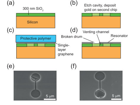 Figure 1
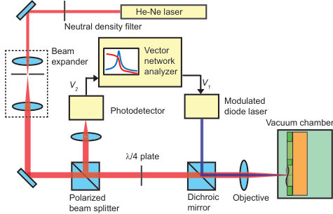 Figure 2
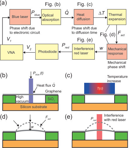 Figure 3
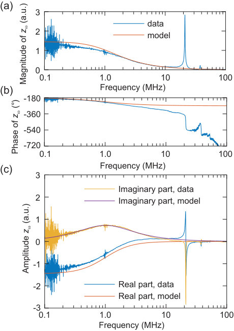 Figure 4
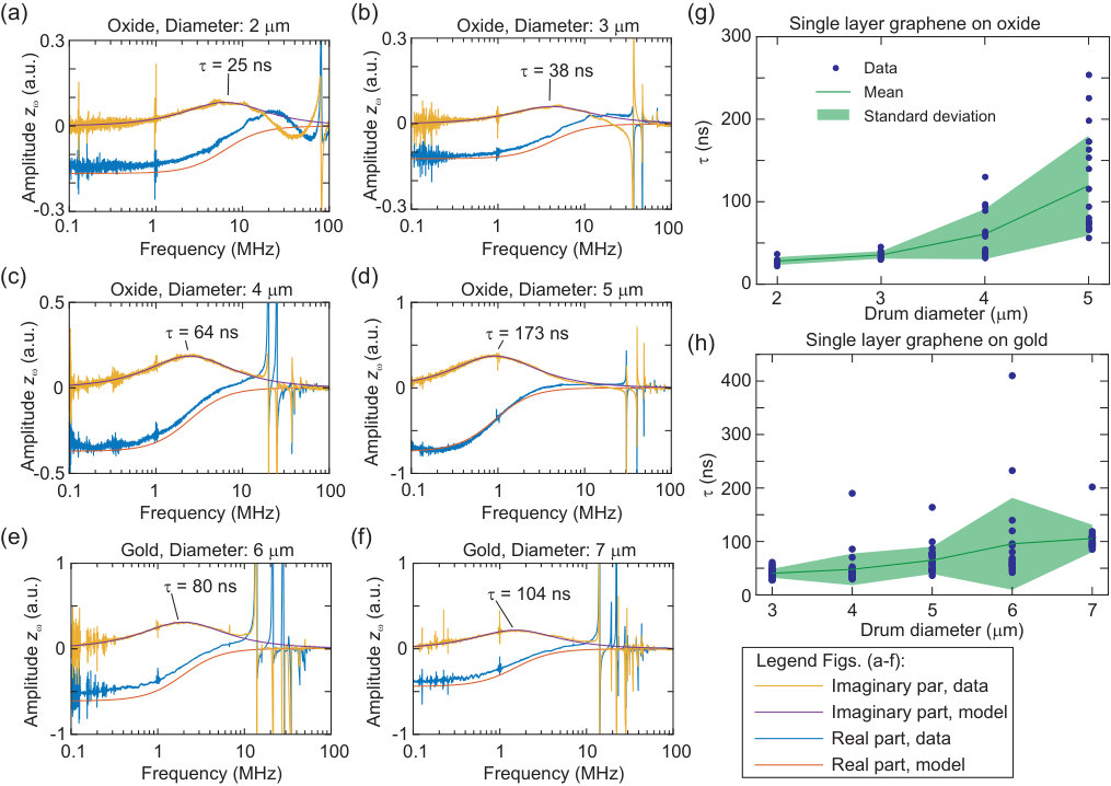 Figure 5
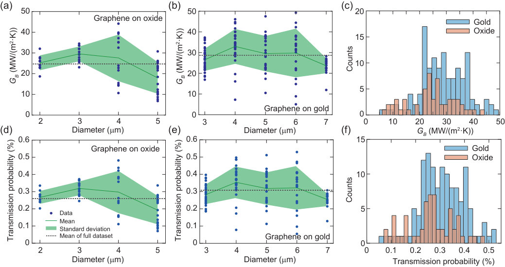 Figure 6
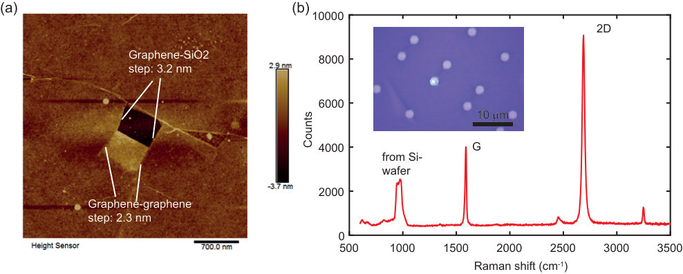 Figure 7
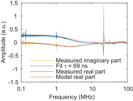 Figure 8
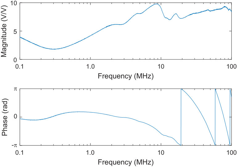 Figure 9
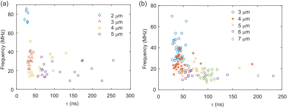 Figure 10
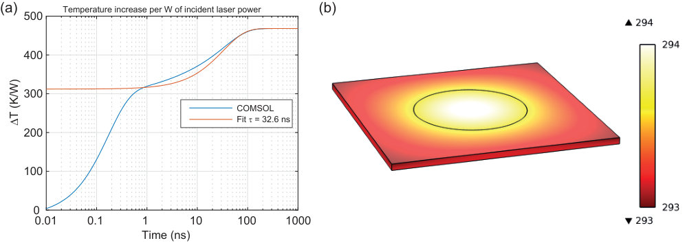 Figure 11
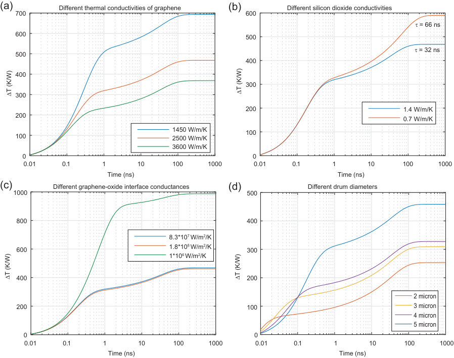 Figure 12
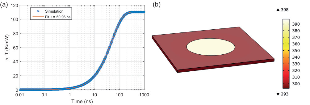 Figure 13
Peer Reviews
No public reviews on file for this paper yet. If you reviewed it on a platform where reviews are public (OpenReview, ICLR, NeurIPS, ICML), you can paste yours below so the community can read it here.
Videos
No videos yet. Explain this paper in a talk, walkthrough, or lecture? Add one.
\useunder
\ul
Optomechanics for thermal characterization of suspended graphene
Robin J. Dolleman
Samer Houri
Dejan Davidovikj
Santiago J. Cartamil-Bueno
Yaroslav M. Blanter
Herre S. J. van der Zant
Peter G. Steeneken
Kavli Institute of Nanoscience, Delft University of Technology, Lorentzweg 1, 2628 CJ, Delft, The Netherlands
Kavli Institute of Nanoscience, Delft University of Technology, Lorentzweg 1, 2628CJ, Delft, The Netherlands
Abstract
Thermal properties of suspended single-layer graphene membranes are investigated by characterization of their mechanical motion in response to a high-frequency modulated laser. A characteristic delay time between the optical intensity and mechanical motion is observed, which is attributed to the time required to raise the temperature of the membrane. We find, however, that the measured time constants are significantly larger than the predicted ones based on values of the specific heat and thermal conductivity. In order to explain the discrepancy between measured and modeled tau, a model is proposed that takes a thermal boundary resistance at the edge of the graphene drum into account. The measurements provide a noninvasive way to characterize thermal properties of suspended atomically thin membranes, providing information that can be hard to obtain by other means.
Graphene is a 2-dimensional material with a honeycomb lattice consisting of carbon atoms Geim and Novoselov (2007). Amongst its many unusual properties, its thermal conductance has attracted major attention Pop et al. (2012); Xu et al. (2016). Extremely high thermal conductivities have been demonstrated up to 5000 W/(mK), well exceeding the thermal conductivity of graphite Balandin et al. (2008); Ghosh et al. (2008). These measurements were performed by Raman spectroscopy, that uses the temperature dependence of the phonon frequency Calizo et al. (2007). By measuring the thermal resistance , which is the local temperature increase per unit of heat flux , one can employ analytical models of the heat transport to extract the thermal conductivity of graphene . This method allowed demonstration that the thermal conductivity decreases when the number of graphene layers is increased from 2 to 4 Ghosh et al. (2010). The method has been subsequently improved, for example by better calibration of absorbed laser power Cai et al. (2010) or removing parallel conduction paths through the air Chen et al. (2010). Also the amplitude ratio between Stokes and anti-Stokes signals has been exploited Faugeras et al. (2010) as an alternative to the shift in phonon frequency. As an alternative to Raman measurements, electrical heaters Xu et al. (2014a), pump probe methods Schwarz (2016); Cabrera et al. (2015), scanning thermal microscopy Yoon et al. (2014) and temperature sensors Seol et al. (2010) have been used to study heat transport in graphene, demonstrating length dependence of the thermal conductivity Xu et al. (2014a) and a reduced thermal conductivity when graphene is supported on silicon dioxide rather than freely suspended Seol et al. (2010). Different groups have demonstrated a large variety in thermal conductivity of graphene between 600 to 5000 W/(mK) experimentally Balandin et al. (2008); Ghosh et al. (2008); Cai et al. (2010); Chen et al. (2010); Faugeras et al. (2010); Xu et al. (2014a); Lee et al. (2011); Dorgan et al. (2013); Chen et al. (2012); Li et al. (2014); Nika and Balandin (2016) and between 100 to 8000 W/(mK) theoretically Nika and Balandin (2016) making the thermal conductance of graphene a debated subject.
Besides these steady-state studies of the thermal properties of graphene, it is of interest to study its time-dependent thermal properties. This requires measurement of small temperature fluctuations in suspended graphene at frequencies in the MHz range. However, since suspended integration of temperature sensors poses problems and optical techniques for temperature measurement in suspended graphene like Raman do not offer the temperature resolution and frequency bandwidth, direct high-frequency temperature measurement in suspended graphene is difficult.
In this work, it is therefore proposed to use the thermomechanical response of suspended graphene to characterize its thermal properties at MHz frequencies. It is found that the mechanical motion is delayed by a characteristic thermal time constant with respect to the intensity-modulation of the laser that opto-thermally actuates the membrane. This is attributed to the time necessary for heat to diffuse through the system. The optomechanics thus provides a tool for studying the dynamic thermal properties of 2D materials. Interestingly, it is found that the measured values of are much higher than those expected based on literature values for the thermal conductivity , specific heat and density of graphene. Models and measurements of drums of different diameters and on different substrates are analyzed in order to account for the large value of . It is found that the long characteristic time is best explained by a large thermal boundary resistance at the edge of the drum.
Single-layer graphene resonators are fabricated on top of 300 nm deep dumbbell-shaped cavities (see Fig. 1). Two substrates are used, one with the cavities etched in a layer of silicon dioxide and the graphene directly transferred on top. The second substrate is coated with a layer of 5 nm chromium and 40 nm gold before graphene is transferred. This is done to help determine whether the thermal properties of the substrate influence the measured characteristic thermal time. Single layer graphene grown by chemical vapor deposition is transferred over both chips covered with a protective polymer. This polymer is dissolved and the sample is dried using critical point drying (CPD) with liquid carbon dioxide. The fluid forces in this process break one half of the dumbbell, creating a resonator on the other half with a venting channel that lets gas below the membrane escape when the vacuum chamber containing the sample is purged. The graphene is further characterized by Raman spectrocopy and atomic force microscopy (AFM) to confirm it is single layer and contamination levels are low (see Supporting Information S1).
The interferometric setup shown in Fig. 2 is used to actuate the membrane and detect the motion Bunch et al. (2007); Dolleman et al. (2015, 2016); Castellanos-Gomez et al. (2013); Zande et al. (2010). In this setup the samples are mounted in a vacuum chamber with optical access. Graphene’s motion is detected by cavity optomechanics using a red He-Ne laser, where the suspended membrane acts as moving mirror and the bottom of the cavity as a fixed back-mirror in a low-finesse Fabry-Perot cavity. The intensity of the blue laser is modulated and heats up the membrane, which will deflect due to thermal expansion. A vector network analyzer (VNA) measures the transmission between the modulation and the signal on the photodetector in a homodyne detection scheme. Frequencies between 100 kHz and 100 MHz can be measured in this setup. All measurements are performed at pressures lower than 0.02 bar, reducing gas damping and heat transport through the gas. The red laser power was 1.2 mW incident on the sample and the blue laser power was at 0.36 mW with a large power modulation of 67% in all experiments.
Here we identify the potential source for time delay between the modulation of the blue laser and the mechanical response in the measurement setup. The block diagram in Fig. 3(a) identifies the elements and processes that play a role in actuation and detection of the membrane’s motion. The modulated intensity of the blue laser is absorbed in the graphene, generating a virtually instantaneous heating power (Fig. 3(b)) since photoexcited carriers in graphene lose their energy to phonons on timescales of a few picoseconds Wang et al. (2010). The generated heat will increase the temperature of the membrane and flow toward the substrate, resulting in a time-dependent temperature increase of the membrane, where the temperature is delayed with respect to the heating power (Fig. 3(c)). The temperature increase causes thermal expansion forces that deflect the membrane (Fig. 3(d)). At frequencies far below the resonance frequency the motion will be in-phase with the thermal expansion force, especially since the quality factor of the resonanator is typically higher than 100. The intensity modulation of the red laser due to interference effect that is used to detect the motion (Fig. 3(e)) can be regarded as instantaneous and will not cause a delay. The measurements are corrected for other delays, related to delays in the instruments (VNA, photodiode) and light path delays, using a calibration procedure discussed in the Supporting Information S3.
It is thus concluded that in the frequency range below the mechanical resonance, the delay between optical actuation and deflection in Fig. 3 is nearly completely due to the delay between heating power and temperature. A thermal system with a single time constant , driven by an ac heating power can be described by the heat equation:
[TABLE]
where is the temperature difference with respect to the steady-state temperature, is the thermal capacitance and is the thermal product. At frequencies significantly below the mechanical resonance frequency, the thermal expansion induced amplitude is proportional to temperature by an effective thermal expansion coefficient . Solution of the heat equation gives:
[TABLE]
In section S6 of the Supporting Information a full derivation of the complex amplitude , including the mechanical damping and inertia effects, is given based on derivations by Metzer et al’ Metzger et al. (2008); Metzger and Karrai (2004); Favero et al. (2007). This equation will be used to fit the experimental data, with the parameters and .
An example of the measured magnitude and phase of the deflection for a resonator with a diameter of 5 m on a cavity in silicon dioxide is shown in Fig. 4(a) and 4(b) respectively. In the 0.1 to 10 MHz range, the response is frequency dependent with a decrease in magnitude as the frequency increases. Also a phase delay is observed that increases as function of frequency. Note, that the measured phase at low frequencies is not 0, but 180 degrees. This is attributed to the small offset in the deflection that the graphene membrane has, in some membranes this was reversed in sign (indicated by 0 degrees phase at low frequencies) as shown in the Supporting Information S2. Figure 4(c) shows a measurement result which is split into a real and an imaginary part. The imaginary part of the amplitude can be fit by eq. 2, resulting in a value of characteristic delay time of ns, with a clearly observable maximum at radial frequency . The real part of eq. 2, with the same and , is shown in Fig. 4(c) showing a small offset with respect to the data. The offset is attributed to optical cross-talk from the modulated blue laser, which can reach the photodetector despite the optical isolation. The same effect causes the difference between the model and the magnitude and phase of the amplitude response (see Figs. 4(a) and 4(b)).
Figs. 5(a-f) show typical measurement results for drums with diameters from 2-7 m. The optical cross-talk is significantly higher in the substrates coated with gold, which is visible as a larger offset in the real part. The resulting values of as function of diameter for both the silicon dioxide substrate and the gold substrate are plotted in Figs. 5(g,h), respectively. A trend is observed where increases as function of diameter. No significant correlation between and fundamental resonance frequency was found as shown in the Supporting Information S4, suggesting weak dependence of on strain.
The measured time constants in this work are significantly larger than expected based on the intrinsic properties of graphene. For example, Barton et al. Barton et al. (2012) use an expression that estimates the time constant based on the thermal properties of graphene:
[TABLE]
where is the membrane radius, the density of graphene, specific heat and the thermal conductivity. Using approximate values J/(kgK) (calculated in the Supporting Information S7), W/(mK) and kg/m3 we obtain ns for a 2 micron drum and ns for a 5 micron drum. The observed values of range between 25 to 250 ns, which is one to two orders of magnitude larger than those predicted by eq. 3. Even if the most extreme values for and are used, eq. 3 gives a lower than measured. The theoretical limit for is given by the Petit-Dulong law ( J/kg/K), and the lowest experimental literature value for is 600 W/(mK) Faugeras et al. (2010). It thus appears that eq. 3 cannot account for the experimental .
Therefore we consider the possibility that the thermal conduction is limited by the substrate that supports the graphene resonator. In order to investigate this, we compare the results obtained on gold-coated and uncoated substrates. It is found that the on the different substrates are similar (Fig. 5(g-h)), despite the much higher thermal conductivity of the gold-coated substrate. It is thus concluded that substrate effects are not responsible for the observed value of . This conclusion is consistent with finite element simulations (Supporting information S5) of the system.
It is well known that a thermal resistance can be present at the interface between two solids Pollack (1969); Stevens et al. (2007); Swartz and Pohl (1989); Peterson and Anderson (1973); Costescu et al. (2003); Lyeo and Cahill (2006). This effect is called interfacial thermal (or Kapitza) resistance and is caused by differences in the phonon velocities, which leads to scattering that limits the phonon transport across the interface. Several works have predicted interfacial resistances in graphene using molecular dynamics simulations Pei et al. (2012); Xu et al. (2014b). Between suspended and supported graphene a value of the boundary conductance of W/(Km2) was reported Xu et al. (2014b). Also, grain boundaries in graphene have been shown to cause an interfacial thermal resistance Isacsson et al. (2016). Below we argue that an interfacial thermal resistance between supported and suspended graphene could account for the unexpectedly long thermal delay times we measured.
The boundary resistance will cause the formation of a temperature discontinuity at the interface between suspended and supported graphene that can be modeled by Fourier’s law Stevens et al. (2007):
[TABLE]
where is the boundary heat flux, the temperature in the suspended part of the graphene and temperature of the supported part. is the thermal boundary resistance and is the thermal boundary conductance. In order to estimate we use a thermal RC model, where the thermal time is given by de product of the heat capacity of suspended graphene and the thermal resistance . It is assumed that is dominated by the interfacial thermal resistance , such that becomes independent of of graphene:
[TABLE]
[TABLE]
where is the thickness of single layer graphene. Combining both expressions yields for the thermal time :
[TABLE]
Using eq. 7 the thermal boundary conductance () is derived from the measurements of as shown in Fig. 6(a), 6(b) and 6(c). This shows that the value of the thermal boundary conductance lies around 30 MW/(mK). For the purpose of extracting the derived value J/(kgK) is used and a density kg/m3. Equation 7 has been verified using finite element simulations that include a thermal boundary conductance, confirming the validity of neglecting the heat conductance (Supporting Information S5).
In order to relate the derived value of to the phonon transmission probability across the interface, the following expression is derived in Supporting Information S7:
[TABLE]
Here is the velocity of the -th phonon mode, for the flexural (ZA), for longitudinal (LA) and for the transverse (TA) mode. The number 1 corresponds to the suspended material. is the integrated transmission probability (the sum over each possible angle of incidence) of phonons over the interface, is Boltzmann constant, is temperature, the reduced Planck’s constant and is the area of the unit cell of graphene.
By using eq. (8), an average phonon transmission probability is plotted in Figs. 6(d), 6(e) and 6(f) corresponding to the boundary conductances in Figs. 6(a), 6(b) and 6(c). The average phonon transmission probability is found to be %. Potential mechanisms that limit include phonon interface scattering due to differences in phonon propagation velocities, boundary roughness Wen et al. (2009) and kinks Evans and Levine (2013) due to graphene edge adhesion Bunch et al. (2008). Further experimental and theoretical study of heat transport across the edge between suspended and supported graphene is needed to clarify the microscopic origins of these observations.
To summarize, a dynamic optomechanical method to measure transient heat transport in suspended graphene is demonstrated. The method does not require electrical contacts, which allows high-throughput characterization of arrays of devices. The method is used to characteristic the thermal time of many graphene membranes. It is found that is a function of diameter and its value is much larger than expected based on existing models. Measurements on gold-coated and uncoated silicon dioxide samples show similar results, showing that cannot be attributed to the substrate. A potential cause for the large values of is the presence of an interfacial thermal resistance between the suspended and supported graphene. From the measurements we determine that a thermal boundary conductance with values of MW/(mK) can account for the measurements, corresponding to a low phonon transmission probability on the order of 0.3%.
Acknowledgments
We thank Applied Nanolayers B.V. for supply and transfer or single-layer CVD graphene on our substrates. We also acknowledge useful discussions with Teun Klapwijk, Debadi Chakraborty, Daniel Ladiges and John Sader. Further, we thank the Dutch Technology Foundation (STW), which is part of the Netherlands Organisation for Scientific Research (NWO), and which is partly funded by the Ministry of Economic Affairs, for financially supporting this work. The research leading to these results also received funding from the European Union’s Horizon 2020 research and innovation programme under grant agreement No 649953 Graphene Flagship and this work was supported by the Netherlands Organisation for Scientific Research (NWO/OCW), as part of the Frontiers of Nanoscience program.
Supplemental Information
Supplemental Information: Optomechanics for thermal characterization of suspended graphene Robin J. Dolleman
Samer Houri Dejan Davidovikj Santiago J. Cartamil-Bueno Yaroslav M. Blanter Herre S. J. van der Zant Peter G. Steeneken
I Additional Experimental results and methods
S1: Graphene characterization
The graphene was examined for contamination and defects using atomic force microscopy (AFM) and Raman spectroscopy. Figure S1(a) shows a height profile obtained using tapping mode AFM on graphene supported on silicon dioxide. A small part of the graphene sheet is broken and folded over, allowing to measure the step heights between graphene on graphene and graphene on silicon dioxide. The tapping mode AFM can overestimate the step height when measuring 2D materials Nemes-Incze et al. (2008). This inaccuracy is illustrated by the disparity between the graphene-oxide and the graphene-graphene step height. However the folded-over part of the graphene allows us to say that no more than 1.9 nm of uniform polymer contamination could be present on the membrane. This value represents a worst-case scenario and it is very likely that the contamination is much lower. The ratio between the 2D and G peak of 2:1 in the Raman spectroscopy (see Fig. S1(b)) and the absence of a D-peak is consistent with high-quality single layer graphene with low contamination levels Ferrari et al. (2006).
S2: Example of measurement with reversed phase
In the main text it is mentioned that the response of the drum can show either a 180 degrees phase shift between laser power and mechanical motion at low frequencies, but also a 0 degrees phase is possible. This is equivalent to a sign change of the real and imaginary part of the amplitude. Although 180 degrees is usually observed in our measurements, occasionally a 0 phase is observed as shown in Fig. S2. Here, the sign of real and imaginary part have changed with respect to the examples in the main text. The cause of this difference in phase are small asymmetries in the initial state which will cause either upward or downward motion due to the thermal expansion.
S3: Calibration procedure
In order to correct the intrinsic phase shifts in our measurement setup, we directly point the blue laser to the photodiode to obtain an calibration curve for our system (Figure S3). This can be corrected by deconvolution of the measured response with this calibration curve, which is done by expressing the blue laser modulation parameters as a frequency-dependent phasor . Since the calibration was taken at discrete frequencies, a cubic interpolation was used to make sure the frequencies match the ones from the measurement that needs to be corrected. Now one can deconvolve the measured frequency response function using:
[TABLE]
[TABLE]
where is the corrected frequency response function of our measurement.
S4: Correlation between resonance frequency and
Figure S4 shows scatter plots between the resonance frequency and characteristic thermal time extracted from the measurements. Since both the resonance frequency and characteristic thermal time are correlated to diameter, correlations between the two variables should only be determined for the same diameter. We found low correlations close to zero with outliers at -0.24 for the 6 micron diameter drums on gold and 0.14 for the 5 micron diameter drums on gold. The low correlations and the low agreement between different diameters suggests that transient thermal transport is not strongly related to the strain present in the graphene resonators.
II Additional modeling results
S5: Finite element simulations of graphene on a silicon dioxide substrate
In order to examine the impact of the silicon dioxide substrate on the heat transport, we use COMSOL Multiphysics to model the graphene on top of the cavity and estimate the delay function . A simulation result of , where is the incident laser power (assuming absorption of optical power), can be seen in Fig. S5. This simulation predicts that the heat transport is more complex than expected. A very fast increase in temperature is observed with a time constant that is in the order of 0.5 ns. This is followed by a much slower exponential increase in temperature, which can be fitted with a single exponential to obtain a time constant of 32.6 ns. The fast time constant should not be observed in our measurement, since the cut-off frequency MHz is much larger than the bandwidth in our measurements. The slow time constant can be observed in our measurement, since the cut-off is in a measurable frequency range and lower than the resonance frequency. This could be the thermal relaxation time found in the measurements.
Figure S6 shows for different material parameters. From fig. S6(a) we conclude that changes in the thermal conductivity or specific heat of the graphene membrane affect the fast time constant , the slow time constant remains unchanged. We conclude that the observed time constant in our measurements does not depend on the properties of graphene itself. For the thermal contact resistance between the graphene and silicon dioxide interface shown in fig. S6(b), we draw the same conclusion.
Figure S6(c) shows a different situation; if the thermal properties of the silicon dioxide layer are changed, the fast time constant remains unchanged. However, the slow time constant changes a lot, from 32 ns to 66 ns if the thermal conductivity is changed from 1.4 W/m/K to 0.7 W/m/K. We therefore conclude that the slow time constant in the simulation depends only on the properties of the substrate. Due to the poor thermal properties of this layer, it takes much longer to reach thermal equilibrium than expected if only the graphene itself is considered. Figure S6(d) shows the diameter dependence on , again the slow time constant is hardly affected, therefore this model does not account for the diameter dependence in our measurement. Since the slow time constant modeled here only depends on the properties of the substrate, it should significantly change value when the silicon dioxide is replaced with gold. Since the values simulated here are not diameter dependent, this model shows that the experimental observations cannot be explained by the thermal properties of the substrate.
Figure S7 shows a simulation with identical parameters as in Fig. S5 with the addition of a limited thermal boundary conductance 40 MW/(m K). The interfacial thermal resistance dominates the heat transport in this situation as illustrated by the uniform temperature in the drum. The materials outside the drum do not raise in temperature significantly. This validates the simple model in the main part of this work, where only the boundary conductance is considered.
S6: Derivation of expression for motion of drum actuated by modulated laser
The derivations below follow the methods used by Metzger et al.Metzger et al. (2008); Metzger and Karrai (2004); Favero et al. (2007) closely. The derivation is repeated here to show that the use of a separate red laser to read out the motion does not affect the amplitude response. We assume there is a weakly intensity-modulated laser actuating the graphene membrane, the force induced by this laser can be written as:
[TABLE]
where is a photo-induced force (which can be photo-thermal, radiation pressure or radiometric pressure) that is exerted on the compliant graphene membrane and a modulation parameter assumed to be much smaller than 1. In general, the graphene membrane will show a delayed response in its deflection due to this force, but responds with a certain time delay . This time-delay can be described by a function that leads to the following formulation for the force:
[TABLE]
In the case of constant illumination, this equation becomes:
[TABLE]
which is valid for the red laser used in the interferometric detection. The combined action of the red and blue laser gives for the total force:
[TABLE]
The equation of motion that needs to be solved now reads:
[TABLE]
where is the amplitude on a generalized coordinate on the membrane, which we assume is the amplitude detected by the red laser; is the effective mass, the effective damping coefficient and the effective stiffness. We drop the term , since this leads only to a static deflection with no time-dependence. We assume that the amplitude is very small and that the terms can be approximated by a constant . Using the properties of Laplace transforms for convolutions we can now write eq. II in the frequency domain:
[TABLE]
We assume the shape of the delay function is of the exponential type:
[TABLE]
which has the Laplace transform:
[TABLE]
Inserting this into the equation of motion gives:
[TABLE]
. Now we split the effective actuation force into where represents the force from the DC blue laser power and is the modulation parameter. is made constant as function of frequency by the calibration method described in section S3. Regrouping in terms of omega gives:
[TABLE]
where we combined and into . The solution for the amplitude is:
[TABLE]
with real and imaginary part:
[TABLE]
In the limit where the imaginary part shows a local maximum at a radial frequency of approximately . In this case, the frequency response function is , which is used in this work to fit to the imaginary part of the measured response.
Derivations of interfacial thermal resistance, specific heat and characteristic thermal time for 2D materials
S7: Derivation of expression for (eq. 8 in main text)
The interfacial thermal resistance can be determined by using the heat flux:
[TABLE]
where is cross sectional area of the boundary, the temperature difference and the heat flux. The first step in determining the interfacial resistance, is thus to determine the heat flux that crosses the interface. The heat flux that crosses from interface 1 to interface 2 can be expressed by Gray (1981); Peterson and Anderson (1973):
[TABLE]
where is the total energy per unit volume of the heat carriers, the velocity at which they propagate and the probability that the heat carriers transmit over the interface. In the calculation of thermal interfacial resistance, the difficulty lies in calculating the transmission probability , while the calculation of energy and propagation velocity is quite straigtforward.
Our approach is thus, to calculate the energy and velocity and use that to estimate the value of from the measurement. In order to do this, it is assumed that the heat in graphene is carried by phonons and that all the heat is carrier by three acoustic phonon polarizations, the longitudinal (LA), transverse (TA) and flexural (ZA). The LA and TA branch are far below the Debye temperature of 2100 K due to their large velocities, but the ZA branch will be fully thermalized since its Debye temperature is at 50 K Hone (2001). The contribution to the heat flux of each polarization can be added to obtain:
[TABLE]
and the total heat flux becomes:
[TABLE]
the index now describes the material ( for suspended, for supported graphene) and phonon mode .
To calculate the energy , we start from the Bose-Einstein distribution to find the average phonon number at a fixed frequency :
[TABLE]
where is the reduced Plack’s constant, the Boltzmann constant and temperature. The energy carried by each phonon is , therefore we can write the average energy that phonons have at this frequency:
[TABLE]
The number of states (density of states ) that is accessible to the system between the frequencies and is defined by:
[TABLE]
and this makes the total energy in the system:
[TABLE]
Next, one has to know for the density of states, how many modes are available in the momentum space. In a 2-dimensional crystal, if we know the size of the system , the uncertainty in momentum is and the number of modes available to the system becomes:
[TABLE]
where one can integrate over circles with circumference to obtain:
[TABLE]
Using we obtain for the total energy in the system:
[TABLE]
which is divided by the total volume of the system to obtain for :
[TABLE]
to perform the integration, it is necessary to use the dispersion relation that relates the frequency to the wavenumber. Since the flexural phonons have different properties than the transverse and longitudinal phonon, these will have to be analyzed separately in the sections below.
II.0.1 Longitudinal and tranverse modes
For the longitudinal and transverse acoustic phonons, we can write the linear dispersion relationship:
[TABLE]
where is the propagation velocity of the phonons, since . Substitution into eq. S27 gives:
[TABLE]
Using this, we can write for the heat flux over an interface of area from material 1 to material 2:
[TABLE]
To solve the frequency integral, we assume and using a coordinate transform :
[TABLE]
We assume that the transmission probability frequency-independent. This results in:
[TABLE]
and for the heat flux from material 2 to material 1:
[TABLE]
II.0.2 Flexural mode
When strain is present in a 2D lattice, the dispersion of the flexural phonons can be written as Lifshitz (1952):
[TABLE]
which has 4 solutions for , however implying the conditions , , and enforcing that must be a real number, we only have one solution:
[TABLE]
this can be substituted in eq. S27 to obtain:
[TABLE]
Note, that this equation converges either to the expression for linear dispersion if or to the expression for quadratic dispersion if . The propagation velocity becomes:
[TABLE]
substituting eq. S35 gives:
[TABLE]
which in the limit case of purely quadratic dispersion becomes and in the case of linear dispersion becomes .
The analysis can be simplified by assuming either high or low strains, which should follow from our experiments. It can be seen, that the condition:
[TABLE]
allows us to use descibe the heat transport of the ZA branch by a quadratic dispersion without strain, while the condition:
[TABLE]
allows one to use a linear dispersion for the ZA branch. From the resonance frequencies in our experiments, we can estimate the strain present in the drum resonators:
[TABLE]
assuming 7.7\text{\times}{10}^{-7} kg/m2 and $Eh=$ 340 N/m, we find the lowest observed strain $\epsilon_{\mathrm{low}}=$1.026\text{\times}{10}^{-5} and the highest observed strain 1.71\text{\times}{10}^{-4}$$. Expressions for coefficients and are given by Lifshitz Lifshitz (1952):
[TABLE]
where is the bending rigidity, which is 1\text{\times}{10}^{-19}$$ J for single-layer graphene, and:
[TABLE]
where is the dilatation and , are the Lame parameters. Now we can calculate the coefficients for the lowest strain:
[TABLE]
[TABLE]
from which we conclude that for each drum measured in this work the condition in eq. S40 holds. Due to the low velocities the Debye temperature of the flexural phonons is much lower than the in-plane phonons. Therefore, we have to write the heat flux as:
[TABLE]
where is the Debye temperature, since we are above the Debye temperature :
[TABLE]
the total number of states in the system is:
[TABLE]
the Debye temperature becomes:
[TABLE]
here is the number of states per unit square, which is limited by the area of the unit cell 5\text{\times}{10}^{-20}$$ m2. The heat flux from the ZA mode now becomes:
[TABLE]
and the total heat flux now becomes:
[TABLE]
The condition has to apply if , this implies that:
[TABLE]
which makes the heat flux:
[TABLE]
This can be linearized for small temperature differences to obtain:
[TABLE]
and the boundary resistance is directly obtained from eq. S16:
[TABLE]
II.0.3 Specific heat
We can also calculate the specific heat by starting from equation S29:
[TABLE]
[TABLE]
which is valid for the LA and TA branches. For the ZA phonons we have to take the high temperature limit:
[TABLE]
using :
[TABLE]
now by substituting:
[TABLE]
the energy density becomes:
[TABLE]
[TABLE]
Now we find:
[TABLE]
[TABLE]
In the main text we found the expression:
[TABLE]
Substituting eqs. S55 and S64 gives:
[TABLE]
this result was used in the main text to estimate the average phonon transmission probability . This average is defined as the situation where all branches have equal transmission probability: .
The reference list from the paper itself. Each links out to its DOI / PubMed record.
- 1Geim and Novoselov (2007) Andre K Geim and Konstantin S Novoselov, “The rise of graphene,” Nature materials 6 , 183–191 (2007).
- 2Pop et al. (2012) Eric Pop, Vikas Varshney, and Ajit K Roy, “Thermal properties of graphene: Fundamentals and applications,” MRS bulletin 37 , 1273–1281 (2012).
- 3Xu et al. (2016) Xiangfan Xu, Jie Chen, and Baowen Li, “Phonon thermal conduction in novel 2d materials,” Journal of Physics: Condensed Matter 28 , 483001 (2016).
- 4Balandin et al. (2008) Alexander A Balandin, Suchismita Ghosh, Wenzhong Bao, Irene Calizo, Desalegne Teweldebrhan, Feng Miao, and Chun Ning Lau, “Superior thermal conductivity of single-layer graphene,” Nano letters 8 , 902–907 (2008).
- 5Ghosh et al. (2008) S Ghosh, I Calizo, D Teweldebrhan, EP Pokatilov, DL Nika, AA Balandin, W Bao, F Miao, and C Ning Lau, “Extremely high thermal conductivity of graphene: Prospects for thermal management applications in nanoelectronic circuits,” Applied Physics Letters 92 , 151911 (2008).
- 6Calizo et al. (2007) I Calizo, AA Balandin, W Bao, F Miao, and CN Lau, “Temperature dependence of the raman spectra of graphene and graphene multilayers,” Nano letters 7 , 2645–2649 (2007).
- 7Ghosh et al. (2010) Suchismita Ghosh, Wenzhong Bao, Denis L Nika, Samia Subrina, Evghenii P Pokatilov, Chun Ning Lau, and Alexander A Balandin, “Dimensional crossover of thermal transport in few-layer graphene,” Nature materials 9 , 555–558 (2010).
- 8Cai et al. (2010) Weiwei Cai, Arden L Moore, Yanwu Zhu, Xuesong Li, Shanshan Chen, Li Shi, and Rodney S Ruoff, “Thermal transport in suspended and supported monolayer graphene grown by chemical vapor deposition,” Nano letters 10 , 1645–1651 (2010).