Potential kernel, hitting probabilities and distributional asymptotics
Francoise Pene, Damien Thomine

TL;DR
This paper develops a generalized central limit theorem for certain dynamical systems, relating hitting probabilities to potential kernels, with applications to Lorentz gases and geodesic flows, expanding theoretical understanding of these systems.
Contribution
It introduces a generalized CLT for Z^d-extensions of dynamical systems, connecting hitting probabilities with potential kernels and improving assumptions for the theorem.
Findings
Proves a generalized CLT under spectral assumptions.
Shows invariance of Green-Kubo's formula under induction.
Relates hitting probabilities to symmetrized potential kernels.
Abstract
Z^d-extensions of probability-preserving dynamical systems are themselves dynamical systems preserving an infinite measure, and generalize random walks. Using the method of moments, we prove a generalized central limit theorem for additive functionals of the extension of integral zero, under spectral assumptions. As a corollary, we get the fact that Green-Kubo's formula is invariant under induction. This allows us to relate the hitting probability of sites with the symmetrized potential kernel, giving an alternative proof and generalizing a theorem of Spitzer. Finally, this relation is used to improve in turn the asumptions of the generalized central limit theorem. Applications to Lorentz gases in finite horizon and to the geodesic flow on abelian covers of compact manifolds of negative curvature are discussed.
Click any figure to enlarge with its caption.
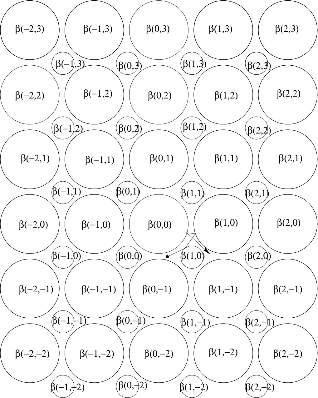 Figure 1
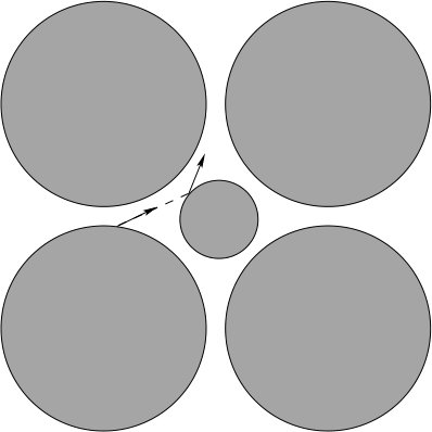 Figure 2
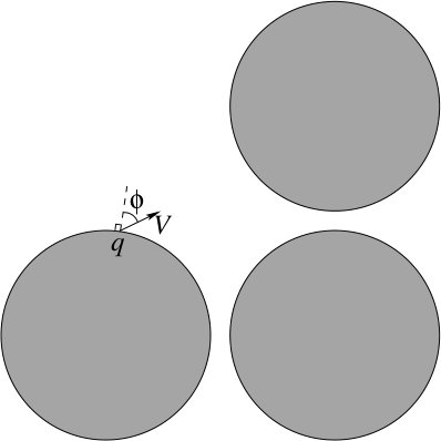 Figure 3
Peer Reviews
No public reviews on file for this paper yet. If you reviewed it on a platform where reviews are public (OpenReview, ICLR, NeurIPS, ICML), you can paste yours below so the community can read it here.
Videos
No videos yet. Explain this paper in a talk, walkthrough, or lecture? Add one.
Potential kernel, hitting probabilities and distributional asymptotics
Françoise Pène
Université de Brest and Institut Universitaire de France, Laboratoire de Mathématiques de Bretagne Atlantique, UMR CNRS 6205, 29238 Brest Cedex, France
and
Damien Thomine
Département de Mathématiques d’Orsay, Université Paris-Sud, UMR CNRS 8628, F-91405 Orsay Cedex, France
Abstract.
-extensions of probability-preserving dynamical systems are themselves dynamical systems preserving an infinite measure, and generalize random walks. Using the method of moments, we prove a generalized central limit theorem for additive functionals of the extension of integral zero, under spectral assumptions. As a corollary, we get the fact that Green-Kubo’s formula is invariant under induction. This allows us to relate the hitting probability of sites with the symmetrized potential kernel, giving an alternative proof and generalizing a theorem of Spitzer. Finally, this relation is used to improve in turn the asumptions of the generalized central limit theorem. Applications to Lorentz gases in finite horizon and to the geodesic flow on abelian covers of compact manifolds of negative curvature are discussed.
Introduction
Given a recurrent random walk on , with , a natural question is how much time the walker spends in any region of the space – the so-called occupation times. More generally, one may choose an observable , and consider the Birkhoff averages . When is summable and the walk is well-behaved, it is known that converges in distribution to a Mittag-Leffler random variable, for well-chosen coefficients [44]. This behaviour generalizes to null-recurrent Markov processes [20, 1].
When has integral zero, this family of results is not sharp enough, and we must look at a higher order. In the same way that a central limit theorem replaces the weak law of large numbers, one can get a generalized central limit theorem for observables of null-recurrent Markov processes. Typically, converges in distribution, with an explicit limit. The story of these central limit theorems starts from Dobrushin [22] where is the simple random walk on . Then these results were generalized to Markov processes [40, 35, 37], and later included invariance principles [36, 9, 10].
In this article, we are interested not in Markov processes, but in a family of dynamical systems preserving an infinite measure: -extensions, which are a generalization of random walks. Starting from a dynamical system preserving a probability measure and a function , we work with the transformation on . This class of systems include random walks on , as well as, for instance, Lorentz gases [14, 13] and the geodesic flow on abelian covers of complete manifolds [38, 57, 52]. Given an observable , we want to understand the limit in distribution of .
In two previous works by the second-named author [63, 64], adapting previous methods [17, 18, 19], the case where is a Gibbs-Markov map was investigated. In the current article, we are able to get a generalized central limit theorem under spectral hypotheses on the transfer operator of the system , which has much wider applications. The downside is that we need the observable to depend only on and decay fast enough at infinity. This is Theorem 1.4, which we prove using the method of moments (an approach which, to our knowledge, is new for this problem), and apply to Lorentz gases with finite horizon.
An interesting corollary of Theorem 1.4 and [64, Theorem 6.8] is that, for -extensions of Gibbs-Markov maps, Green-Kubo’s formula – which appears as the asymptotic variance in the central limit theorem – is invariant under induction. This is the content of Corollary 1.13. By choosing the observable carefully, in Theorem 1.7 we are able to related the probability that an excursion from hits a site , and the symmetrized potential kernel associated to the -extension. Our proof relies on the first hitting time of small target statistics. This method provides a new proof of an earlier proposition by Spitzer [59, Chap. III.11, P5], and generalizes it to -extensions (for which harmonic analysis as used in [59] does not make sense). Finally, the estimates from Theorem 1.7 are used to relax the assumptions from [64]: in Theorem 1.11, the observables need only to decay polynomially at infinity, instead of having bounded support. We apply it to the geodesic flow on abelian covers of compact manifolds with negative curvature.
This article is organized as follow. We present our setting and our results in Section 1, as well as our applications to Lorentz gases (Sub-subsection 1.4.1) and to geodesic flows (Sub-subsection 1.4.2). In Section 2 we present our spectral assumptions, and prove Theorem 1.4 using the method of moments. In Section 3 we prove Theorems 1.7 and 1.11, and in Section 4 the two applications mentioned above. We discuss Green-Kubo’s formula in the Appendix.
Acknowledgements
The second author is indebted to Sébastien Gouëzel, both for it guidance during his PhD and for his discussions on the subject, as well as to Péter Nándori for suggesting part of the argument of Section 3.
We also wish to thank the Erwin Schrödinger Institute for the program “Mixing flow and averaging methods” (Vienna, 2016), the CNRS for the grant PEPS “Moyennisation et analyse stochastique des systèmes lents-rapides” (2016), and the IUF for their support.
1. Main results
1.1. Setting and goals
We consider conservative ergodic dynamical systems given by -extensions of probability-preserving dynamical systems, where the underlying dynamical system is sufficiently hyperbolic and . We shall deem a system hyperbolic enough if its transfer operator satisfies good properties. For some applications, we use the stronger assumption that the underlying dynamical system is Gibbs-Markov.
Let be a probability-preserving dynamical system. Let with be a -integrable function such that . The -extension of with step function is the dynamical system given by:
- •
;
- •
;
- •
.
Note that preserves the infinite measure . We shall always assume that is ergodic. If has a Markov partition , we may also asume that the step function is -measurable – that is, constant almost everywhere on elements of the partition. We then say that is a Markov extension of .
Let be the second coordinate of . Heuristically, the sequence , under the distribution , behaves much like a random walk, the randomness being generated by the dynamical system . Indeed, this family of extensions includes every random walk on , as well as some physically or geometrically interesting systems such as Lorentz gases (Sub-subsection 1.4.1) or the geodesic flow on -periodic manifolds of negative curvature (Sub-subsection 1.4.2) 111Up to some lengthy, but in our case not particularly challenging, legwork to go from discrete time to continuous time..
In the present paper, we will make assumptions ensuring the convergence in distribution of to a Lévy stable distribution, for some normalizing sequence . Our main goals are the following:
- (A)
Given integrable and such that , we are interested in the asymptotic behaviour of the ergodic sum
[TABLE]
as . More precisely, we are looking for a non-trivial strong convergence in distribution:
[TABLE]
where is some constant which depends on the pushforward of the measure by , whereas the random variable depends only on222Up to a constant, actually depends only on the index of the Lévy stable distribution that is the limit of . the distribution of (with respect to ).
- (B)
In the context of Gibbs-Markov maps, we consider the probability , starting from the endowed with the measure , to visit before coming back to . By applying the limit theorems we have proved before to , we are able to prove that
[TABLE]
which provides a new proof of [59, Chap. III.11, P5], and generalizes it to systems which are not random walks.
The next sub-sections present in more details these two goals, and the precise statements we get.
1.2. Distributional limit theorems
1.2.1. Convergence and limit distributions
When working with spaces endowed with an infinite measure, there is no natural notion of convergence in distribution. We shall instead use the notion of strong convergence in distribution. The reader may consult e.g. [1, Chapter 3.6] for an introduction to this notion and applications to ergodic dynamical systems whose invariant measure is infinite.
Definition 1.1** (Strong convergence in distribution).**
Let be a measured space. Let be a sequence of measurable functions from to . Let be a real-valued random variable. We say that converges strongly in distribution to if, for all probability measures ,
[TABLE]
Now that we have defined our mode of convergence, we introduce our limit objects: Mittag-Leffler random variables, and Mittag-Leffler – Gaussian mixtures.
Definition 1.2** ( and random variables).**
Let . Let be a non-negative real-valued random variable. We say that follows a standard Mittag-Leffler distribution of index if, for all (or all if ),
[TABLE]
If this is the case, we shall write that has a distribution.
Let be a real-valued random variable. We say that follows a standard Mittag-Leffler – Gaussian mixture distribution of index if , where and are two independent random variables with respective distribution and standard normal . If this is the case, we shall write that has a distribution. See [62, Chapitre 1.4] for a partial description of the MLGM distributions.
For , these distributions take more common forms: a distribution is an exponential distribution of parameter , while a distribution is a Laplace distribution of parameter . A random variable is the absolute value of a centered Gaussian of variance .
1.2.2. Main distributional theorem
Mittag-Leffler distributions appear when one studies the distributional convergence of the local time of null recurrent Markov processes, or chaotic enough -finite ergodic dynamical systems. For the Brownian motion, the result goes back to P. Lévy [44], and to Darling-Kac’s theorem for Markov chains [20]. We refer the reader to [46] for -stable Lévy processes, and to [1, Corollary 3.7.3] for dynamical systems in infinite ergodic theory. For instance [1, Corollary 3.7.3] and Hopf’s ergodic theorem [31, §, Individueller Ergodensatz für Abbildungen] yield:
Proposition 1.3**.**
Let be a measure-preserving transformation of a -finite measure space. Assume that is pointwise dual ergodic with return sequence (see [1, Chapter 3.5] for definitions). Assume that has regular variation of index , i.e. for some sequence which varies slowly at infinity. Then, for all ,
[TABLE]
where is a standard random variable and the convergence is strong in distribution.
However, this kind of result is not sharp enough when the integral of the observable is zero. We want to get more precise asymptotics, that is to say, some kind of central limit theorem for observables of -finite ergodic dynamical systems whose integral is [math]. We need to add some regularity condition on the observable , as well as stronger integrability conditions – as is usual in ergodic theory, for instance to get a central limit theorem [47, 48]. In this article, we shall prove the following result:
Theorem 1.4**.**
Let be an ergodic and aperiodic -extension of with step function and . Assume Hypothesis 2.1. Let be an -regularly varying sequence of positive numbers and be an -stable random variable such that
[TABLE]
Let . Let be such that:
- •
* for some ;*
- •
.
Let . Then the following sums over are absolutely convergent:
[TABLE]
Moreover,
[TABLE]
where is a standard random variable and the convergence is strong in distribution, and where is the continuous version of the density function of .
Under the hypotheses of Theorem 1.4, we have in addition:
[TABLE]
Remark 1.5**.**
For a definition of aperiodicity, see Definition 3.9. It is not necessary in the statement in the theorem, but appears as a result of Hypothesis 2.1, and we prefer to make this assumption explicit.
We do not expect aperiodicity to be necessary in the statement of Theorem 1.4, up to the necessary modification in Hypotheses 2.1. Proving this generalization would be straightforward if were allowed to depend on ; however, allowing such a dependence would make the proof of Theorem 1.4 much more difficult. We choose to leave the non-aperiodic case aside, except for a couple of later results, Theorem 1.7 and Theorem 1.11.
Theorem 1.4 shall be proved in Section 2 with the method of moments and is based on refinements of the local limit theorem for , which says that . Under our hypotheses, the normalization is equivalent to . See e.g. [4] for a spectral proof of the local limit theorem, which holds under Hypotheses 2.1, and implies the equivalence of the normalizations.
In special cases, the normalization can be made explicit:
[TABLE]
1.2.3. Symmetrized potential kernel
The case when of Theorem 1.4 is especially interesting. Then the computation of boils down to an estimation of the symmetrized potential kernel of the -extension:
[TABLE]
with
[TABLE]
which is well defined under the assumptions of Theorem 1.4. We estimate the asymptotic growth of in Subsection 2.5, adapting the methods of [59] to dynamical systems. We get:
Proposition 1.6**.**
Let be an ergodic, aperiodic -extension of with step function . Let be a complex Banach space of functions defined on . Assume Hypothesis 2.1 holds with and . If , let be the functions defined by Equation (2.58).
If and ,
[TABLE]
If ,
[TABLE]
If ,
[TABLE]
1.3. Hitting probabilities of excursions
We leave aside for a moment the distributional asymptotics of the Birkhoff sums, and focus on the probability that an excursion hits a given site (Section 3). We now assume that is a Gibbs-Markov map. The leading theme of this section is the study of the probability that an excursion from hits , and its asymptotics as goes to infinity.
1.3.1. Induced transformations
Let us describe the terminology. We define , where is the length of an excursion starting from :
[TABLE]
Then, define the corresponding induced map by , which is well-defined for almost every . Note that is a measure-preserving ergodic dynamical system [33]. For any observable , let:
[TABLE]
Let us introduce a few more objects: the time that an excursion from spends at , and the inverse probability that an excursion from hits , and the number of times that the system goes back to before hitting . Formally,
[TABLE]
[TABLE]
and:
[TABLE]
The following theorem explains how these quantities are related in the limit .
Theorem 1.7**.**
Let be a conservative and ergodic333The extension need not be aperiodic for this theorem. Markov -extension of a Gibbs-Markov map . Then:
- •
As ,
[TABLE]
- •
The conditional distributions have exponential tails, uniformly in : there exist and such that, for every ,
[TABLE]
- •
* converges in distribution and in moments to an exponential random variable of parameter as goes to infinity. In particular, for all ,*
[TABLE]
The proof of Theorem 1.7 rests on two main points: the exponential tightness of (Subsection 3.3), and its convergence to an exponential random variable (Subsection 3.4). The later point is an interesting application of the general fact that, for many hyperbolic dynamical systems, the hitting time of small balls, once renormalized, converges in distribution to an exponential random variable (see e.g. the reviews [16, 56, 29]). Once we have tightness and convergence in distribution, we can evaluate the moments of .
For random walks, many estimates are more explicit. For instance, the distribution of is geometric, so its moments are exactly known (as functions of ). With this improvement, one can recover part of [59, Chap. III.11, P5] – that is, the equivalents in Theorem 1.7 and Corollary 1.9 can be made into equalities:
[TABLE]
1.3.2. Induction invariance of the Green-Kubo formula
While Theorem 1.7 gives asymptotic relationships between many quantities, it does not provide any way to effectively compute them. For random walks, and are related through a probabilistic interpretation of the symmetrized potential kernel:
Proposition 1.8**.**
[59, Chap. III.11, P5]**
Consider an ergodic aperiodic random walk on . For all ,
[TABLE]
We are able to generalize this proposition to a larger class of dynamical systems. To our knowledge, our proof of Proposition 1.8 is new even for random walks. We leverage Theorem 1.4 and [64, Theorem 6.8]. Whenever the hypotheses of theses theorems coincide, their conclusions must be the same. Hence, the scaling factors before the distribution must be the same, that is,
[TABLE]
If we apply this observation to , we get:
Corollary 1.9**.**
Let be an aperiodic Markov -extension of a Gibbs-Markov map with step function . Assume that the extension is ergodic, conservative, and either of the following hypotheses:
- •
* and is in the domain of attraction of an -stable distribution, with .*
- •
* and at [math], for some real numbers and and some function with slow variation.*
- •
* and is in the domain of attraction of a non-degenerate Gaussian random variable.*
Then, as ,
[TABLE]
Remark 1.10** (-stable laws).**
The description of the distributions in the basin of attraction of a -stable law is notoriously difficult [2]. As in Hypothesis 2.1, we choose to make a spectral assumption. It does not capture all such distributions, but includes e.g. symmetric distributions. We believe that this assumption can be significantly weakened if needed.
1.3.3. An improved distributional limit theorem
Proposition 1.6 provides a first-order estimate of , depending on the tails of . We can use this estimate to run an (improved version of) an argument by Csáki, Csörgő, Földes and Révész [17, Lemma 3.1]. we get more explicit integrability conditions than in [64, Theorem 6.8] for observables of -extensions, which yields a new distributional limit theorem. Note that aperiodicity is not required for this result.
Theorem 1.11**.**
Let be a Markov -extension of a Gibbs-Markov map with step function . Assume that the extension is ergodic, conservative, and either of the following hypotheses:
- •
* and is in the domain of attraction of an -stable distribution, with .*
- •
* and at [math], for some real numbers and and some function with slow variation.*
- •
* and is in the domain of attraction of a non-degenerate Gaussian random variable.*
Let be such that:
- •
the family of function is uniformly locally -Hölder for some ;
- •
* for some and ;*
- •
.
Then:
[TABLE]
where is a standard random variable, the convergence is strong in distribution, and:
[TABLE]
where the limit is taken in the Cesàro sense.
Remark 1.12** (Optimal exponent in the summability assumption).**
We consider the case when and . In [17] and some subsequent works by the same authors, the condition required for is:
[TABLE]
The reason is that the authors used Jensen’s inequality in their proof [17, Lemma 2.1], which is in this context less efficient than Minkowski’s inequality, which we used in the proof of Lemma 3.18. This small modification can be implemented in their proof, which improves by a factor some requirements in their works, e.g. [17, Theorem 1] and [18, Example 3.3].
Finally, the hypotheses of Theorem 1.4 and of Theorem 1.11 have a greater overlap than those of Theorem 1.4 and [64, Theorem 6.8], so we can improve the observation in Equation (1.5):
Corollary 1.13** (Induction Invariance of the Green-Kubo formula).**
Let be an ergodic Gibbs-Markov map. Assume that the step function is -measurable, integrable, aperiodic, and that . We also assume that the distribution of with respect to is in the domain of attraction of an -stable distribution, and that the Markov extension is conservative and ergodic.
Let be such that:
- •
* for some ;*
- •
.
Let . Then:
[TABLE]
See Appendix A for a discussion of this corollary.
1.4. Applications
To finish this introduction, we present some applications of our results to more concrete dynamical systems : the geodesic flow on abelian covers in negative curvature, and Lorentz gases (i.e. periodic planar billiards). The proofs can be found in Section 4.
1.4.1. Periodic planar billiard systems
Lorentz gases – that is, periodic or quasi-periodic convex billiards – are classical dynamical systems, whose initial motivation comes from the modelization of a gas of electrons in a metal. The electron is then seen as bouncing on the atoms of the metal, which act as scatterers.
In the plane and with a finite horizon, Lorentz gases exhibit classical diffusion, and the trajectory of a particle behaves much like a random walk in the Euclidean space. For instance, the trajectories are chaotic [58], satisfy a central limit theorem [14, 13], a local limite theorem [60], an almost sure invariance principle [26] (i.e. the renormalized trajectories converge in a strong sense to the trajectories of a Brownian motion), etc. We refer the reader to [15] for more informations of billiards. While the infinite horizon case is also well-known [61, 21], it presents many non-trivial difficulties, so we shall restrict ourselves to finite horizon planar billiards.
Choose a -periodic locally finite configuration of obstacles , where is a finite set. We assume that the obstacles are convex open sets, with pairwise disjoint closures (so that there is no cusp), that their boundaries are and have non-vanishing curvature. We assume moreover that the horizon is finite: every line in meets at least one obstacle. The billiard domain is the complement in of the union of the obstacles .
We consider a point particle moving at unit speed in the billiard domain , bouncing on obstacles with the classical Descartes reflexion law: the incident angle equals the reflected angle and going straight on between two collisions. This is the billiard flow, whose configuration space is (up to a set of zero measure) . Now, consider this model at collision times; the configuration space is then given by . The space is endowed with the Liouville measure , which has density in with respect to the Lebesgue measure (see the picture), and is invariant under the collision map.
For every , we call cell any set and attribute to this cell a value given by a function . We assume that the particle wins the value associated to each time it touches it. We are interested in the behaviour, as , of the total amount won by the particle after the -th reflection.
We write for the index in of the cell touched at the -th reflection time by a particle starting from . Recall that converges strongly in distribution (with respect to the Lebesgue measure on ) to a centered gaussian random variable with positive definite covariance matrix [14, 13, 65].
If is summable and , then converges strongly in distribution to , where has a non-degenerate exponential distribution. This follows e.g. from [1, Corollary 3.7.3] and Young’s construction [65], and is also done in [21]. In another direction, if is a sequence of independent identically distributed random variables independent of the billiard, the asymptotic behavior of is markedly different [50].
We present two applications of Theorem 1.4, the first for (hidden) -extensions, and the second for -extensions.
Corollary 1.14**.**
With the above notations, assume that:
- •
* for some function ;*
- •
there exists such that ;
- •
.
Then:
[TABLE]
where the convergence is strong in distribution on , the random variable follows standard distribution, and:
[TABLE]
In addition, if and only if is a coboundary.
Corollary 1.15**.**
With the above notations, assume that:
- •
there exists such that ;
- •
.
Then:
[TABLE]
where the convergence is strong in distribution on , the random variable follows a Laplace distribution of parameter , and:
[TABLE]
In addition, if and only if is a coboundary.
1.4.2. Geodesic flow on abelian covers
The geodesic flow on a connected, compact manifold with negative sectional curvature is a well-known example of a hyperbolic dynamical system. The geodesic flow on abelian covers of such manifolds provides a class of dynamical systems which preserve a -finite measure, for instance the Liouville measure. They are also more tractable than billiards, as they do not have singularities. These geodesic flows have been studied by extensively, for instance to count periodic orbits on the basis manifold of given length in a given homology class [38, 57, 52]. There are extensions to Anosov flows [7] as well as to surfaces with cusps [3]. Finally, let us mention that the geodesic flow on periodic manifolds is also used to study the horocycle flow on the same manifolds [6, 41, 42, 43].
Limit theorems for observables with integral zero have already been obtained in this context [64], but the improvement we get with Theorem 1.11 translates into a limit theorem which is valid for a wider class of observables. Instead of having compact support, the observables need only to decay polynomially fast at infinity.
Let be a compact, connected manifold with a Riemannian metric of negative sectional curvature. Let be a connected -cover of . Given a Gibbs measure on , we endow with a -finite measure by lifting locally. We refer the reader to [49, Chapter 11.6] for more details about Gibbs measures in this context.
Let be the geodesic flow on . In Subsection 4.2, we shall prove the following proposition, which is a generalization of [64, Proposition 6.12]:
Proposition 1.16**.**
Let be the lift of a Gibbs measure corresponding to a Hölder potential. Assume that the extension is ergodic and recurrent. Fix . Let be a real-valued Hölder function on . Assume that:
- •
there exists such that ;
- •
.
If , there exists such that:
[TABLE]
where the convergence is strong in distribution on , and follows a standard distribution.
If , there exists such that:
[TABLE]
where the convergence is strong in distribution on , and follows a standard distribution.
In both cases, if and only if is a measurable coboundary.
Remark 1.17** (Recurrent extensions of Gibbs measures).**
Given a Hölder potential , let . We say that the potential is reversible if and are cohomologuous, that is, if there exists a Hölder function such that for all . In this case, we also say that is a Hölder coboundary. We say that a Gibbs measure is reversible if it associated to a reversible potential.
For instance, both the Liouville measure and the maximal entropy measure are reversible, because the associated potentials (constants for the maximal entropy measure, and the log-Jacobian of the flow restricted to the unstable direction for the Liouville measure) are reversible.
If is a reversible Gibbs measure and , then the geodesic flow on is both ergodic and recurrent (see [53] for the constant curvature case, although the proof works as well in variable curvature).
The only difference between Proposition 1.16 and [64, Proposition 6.12] is that the assumption that has compact support is relaxed to for some .
Note that our work gives us more information on this system; for instance, Theorem 1.7 can be adapted to yield an asymptotic equivalence of the probability that, starting from some nice Poincaré section , the geodesic flow reaches a faraway Poincaré section before returning to . However, the geometric interpretation of these sections is less evident than for others systems, such as billiards.
2. Theorem 1.4: assumptions and proof
This Section is mostly devoted to the proof of Theorem 1.4. It is organized as follows. The spectral hypotheses are presented in Subsection 2.1. The following three subsections contain respectively a sketch of the proof of Theorem 1.4, the full proof of the theorem, and a proof of the more technical estimates we use. Finally, in Subsection 2.5 we prove Proposition 1.6.
2.1. General spectral assumptions
Let be the transfer operator associated to , that is,
[TABLE]
We consider the family of operators defined by , where stands for the usual scalar product in . Note that:
[TABLE]
We make the following assumptions. Thanks to perturbation theorems (see namely [47, 48, 27, 39, 30] for the general method, and [4] for an application to Gibbs-Markov maps), they hold for a wide variety of hyperbolic dynamical systems.
Hypothesis 2.1** (Spectral hypotheses).**
The stochastic process is recurrent. There exists an integer and a -essential partition of in measurable subsets such that for all ( if is mixing).
There exists a complex Banach space of functions defined on , on which acts continuously, and such that:
- •
.
- •
* and for every , the multiplication by belongs to , where stands for the Banach space of linear continuous endomorphisms of .*
- •
There exist a neighbourhood of [math] in , two constants and , two continuous functions and such that
[TABLE]
with:
[TABLE]
- •
If , there exists such that, for all ,
[TABLE]
as goes to [math], where for some real numbers and such that if . We set .
- •
If , there exists an invertible positive symmetric matrix such that, for all ,
[TABLE]
as goes to [math], where and is slowly varying at infinity. We set .
Hypothesis 2.1 implies the ergodicity of and the mixing of for all as soon as is dense in . If the system is not mixing, then it is expected that the transfer operators has multiple eigenvalues of modulus . The following proposition asserts that, in this case, the standard spectral techniques yield a decomposition as in Equation (2.2).
Proposition 2.2**.**
Assume the begining of Hypothesis 2.1 and its first two items, and that is mixing. Assume in addition that there exist a neighbourhood of [math] in , two constants and and continuous functions and such that:
[TABLE]
and , with:
[TABLE]
Then , and the equations (2.3), (2.4), (2.5), (2.6), (2.7) are satisfied. If moreover is continuous on and admits no eigenvalue of modulus for , then Equation (2.8) is also satisfied, up to increase of and .
Proof.
Up to taking a smaller , we assume that and . Then for every , and . Hence we can take and, up to a permutation of indices, we assume that with and ( ensures that is an eigenvalue of , and this convention yields Equation (2.5)). Hence , with:
[TABLE]
Note that and that , which proves equations (2.3) and (2.4). In the general case, it remains to prove (2.6).
Let be an eigenvector for the eigenvalue of . For all ,
[TABLE]
so that . Since is mixing, must be constant on each ; using Equation (2.9), we get that is proportional to . We conclude that:
[TABLE]
and from there that .
Finally, Equation (2.8) comes from [4]. ∎
For every , we set
[TABLE]
so that . The sequence is then regularly varying of index . Under Hypothesis 2.1, for every . Thus, the sequence converges in distribution to an -stable random variable with characteristic function .
2.2. Strategy of the proof
Given the length of the proof and the technicality of some of its parts, we give here a brief outline of how the method of moments can be applied to our problem.
The proof consists in showing the convergence for every of the following quantity:
[TABLE]
Hence we have to deal with quantities of the following form:
[TABLE]
where . Let us write for this quantity, which behaves roughly as:
[TABLE]
This equation would actually be exact if were a random walk. Then, put and , so that:
[TABLE]
We prove that
[TABLE]
and even that
[TABLE]
except if is made of s and of pairs of consecutive s and of nothing else, which implies that is even. In particular, for all odd ,
[TABLE]
This is the content of Lemma 2.4, which is by far the most technical part of our proof. This is also the point where we use the fact that has zero sum; otherwise, we would get for .
If is made of s and disjoint pairs of consecutive , then it contains times the value and pairs . Then, we shall prove that:
[TABLE]
where the constants and are explicit and yield the random variables.
2.3. Proof of Theorem 1.4
In this section we prove Theorem 1.4. To prove the strong convergence in distribution, it is actually sufficient to prove the convergence in distribution with respect to some absolutely continuous probability measure [67, Theorem 1]. At first, we prove the convergence of under the probability measure , i.e. the convergence of under the probability measure , where:
[TABLE]
We use the method of moments. Let be an integer, which is fixed for the remainder of this proof. Then, for all :
[TABLE]
We delete the terms which are null, and regroup those which are equal. Let us consider one of the terms . We may assume that as soon as ; otherwise, and the whole product is zero. Let . Then with . We set for the multiplicity of in , and if . We write , and , and set, by convention, and . Observe that
[TABLE]
and that the number of -uplets giving the same pair is equal to the number of maps such that for all . Hence:
[TABLE]
For all , for all and for all such that and , we define:
[TABLE]
so that:
[TABLE]
Instead of working with a sequence of times and positions , it shall be more convenient to work with time increments and position increments. Let . We can describe this sequence with integers by taking and for all . Let be the set defined by:
[TABLE]
Then summing over all such that is the same as summing over all in , whence:
[TABLE]
A single coefficient is the contribution to the th moment of by paths of length and with weights . Our goal is to find a sub-family of such weighted paths which is manageable enough so that we can estimate the behaviour of the , and large enough so that it makes for almost all as goes to infinity. However, in order to benefit from the fact that , we use transfer operators, and a decomposition which leverages this equality to make some further simplifications444If has non-zero integral, different terms dominate, and the moments grow faster. It is thus essential to cancel out these “first order terms”..
For all and , we define an operator acting on by:
[TABLE]
where we used (2.1) to establish the second formula. For , we write:
[TABLE]
Recall that . Hence, by induction,
[TABLE]
Plugging this identity into Equation (2.12) yields:
[TABLE]
We further split the operators . Let us write:
[TABLE]
with:
[TABLE]
which we know is possible thanks to Lemma 2.6.
We introduce these operators and into (2.13), creating new data we need to track: the index of the operator we use at each point in the weighted path. Fix , and . Given and , write:
[TABLE]
so that:
[TABLE]
Now, the main question is: for which data do the coefficients , seen as functions of , grow the fastest? One would want to use the larger operator whenever possible, and to use the lowest possible weights whenever possible (because lower weights means larger value of , so a faster combinatorial growth). A priori, the best possible choice would be and . That is indeed true for observables with non-zero integral. However, in our case, the fact that induces a cancellation, which makes the corresponding coefficient vanish. This can be seen with the following elementary properties.
Properties 2.3**.**
Consider a single linear form . For all , the terms on the right side of depend only on , and the terms on its left side only depend on . Hence:
- (I)
Since does not depend on , the value of does not depend on . Without loss of generality, we shall choose to be [math] when . 2. (II)
* and for all , .* 3. (III)
, i.e.
[TABLE]
since . 4. (IV)
In particular, , and:
[TABLE] 5. (V)
[TABLE] 6. (VI)
Applying Point and the fact that , we get:
[TABLE]
Given a sequence , we can iterate Point above to cut into smaller pieces, for which [math] may only appear at the beginning of the associated sequences of indices, and then use Point to transform the heading . Write for the indices such that . We use the conventions that and , that if , and that an empty product is also equal to . Then:
[TABLE]
We sum over , and get:
[TABLE]
Fix such that , and such that . The control of (2.15) and of (2.16) shall be done with the following technical lemma, the proof of which is postponed until Subsection 2.4.
Lemma 2.4**.**
Under the assumptions of Theorem 1.4 and with the previous notations, for every and , for every ,
[TABLE]
We consider the following condition on the sequences and :
[TABLE]
Note that this condition imply that .
Corollary 2.5**.**
Use the assumptions of Theorem 1.4 and the previous notations. Let , and be such that . If Condition (2.22) holds, then
[TABLE]
otherwise:
[TABLE]
In particular,
[TABLE]
Proof.
Due to Equation (2.17), the term (2.15) is an if , and an if .
Let us now estimate the term (2.16). Due to Equation (2.17), since , for all and , for all ,
[TABLE]
Due to Equation (2.20), this estimate holds when and ; due to Equation (2.21), this estimate holds when and .
The two remaining cases are , and . When and , we have a upper bound in . When , the same upper bound is given by Equation (2.20). If and , then Equation (2.20) yields a upper bound in .
Hence, the term (2.16) is in if, for every , we are in one of two cases:
- •
, and ;
- •
, .
Otherwise, (2.16) is in . In particular,
[TABLE]
Furthermore, if Condition (2.22) is not satisfied, either (2.15) is an or one of the terms in (2.16) is an , so . This is the case, in particular, if is odd. ∎
Condition (2.22) can be rewritten:
- •
;
- •
as soon as ;
- •
there exists such that ;
- •
and for all .
Assume now that is even. Let us write for the set of such that and is the disjoint union of pairs of the form . Given , there exists a unique such that satisfies Condition (2.22). Note that and , so that and . Then:
[TABLE]
Let be the set of -uplets of integers such that . Using Points and in Properties 2.3, we get:
[TABLE]
The sequence has regular variation. Due to Lemma 2.7, for all ,
[TABLE]
Hence, by the dominated convergence theorem,
[TABLE]
If , or but , we have already seen that . Therefore, by Equation (2.11),
[TABLE]
For fixed , the value of does not depend on , as the multiset of weights is the same. There are maps from to such that each have preimages, and each have preimage. Thus,
[TABLE]
For fixed , there are sequences : each such sequence is the concatenation of blocs of two different kinds, with blocs of one kind. Thus, for even ,
[TABLE]
Let be a random variable with a standard distribution. Its distribution function is even, so all its odd moments are [math]. Let have a standard Mittag-Leffler distribution of parameter and be a standard Gaussian random variable. Then the even moments of are:
[TABLE]
so that, for even :
[TABLE]
We already know that for odd . Hence, all the moments of converge to the moments of . Since:
[TABLE]
Carleman’s criterion is satisfied [23, Chap. XV.4], so converges in distribution to , when is endowed with the probability measure .
Finally, remark that:
[TABLE]
so by [67, Theorem 1], the sequence converges strongly in distribution to .
2.4. Technical lemmas
In the previous section, we used three technical lemmas, whose proofs would have been to long to include into our main line of reasoning. Their statements and proofs follow.
We begin with Lemma 2.6, which we used to control each part of the decomposition . Recall that is the continuous version of the density function of the stable distribution with characteristic function . Since for , the following lemma can be understood as a strong form of the the local limit theorem for .
Lemma 2.6**.**
We assume that the Hypotheses 2.1 hold.
Let . For every positive integer ,
[TABLE]
with .
Moreover, for every ,
[TABLE]
and:
[TABLE]
Proof of Lemma 2.6.
Recall that . From Hypothesis 2.1, and up to taking a smaller neighborhood , there exist constants , such that and:
[TABLE]
for all .
Let . Since is slowly varying at infinity and is invertible, by Karamata [34] (or Potter’s bound [8, Theorem 1.5.6]), there exists such that, for every and ,
[TABLE]
Since , up to choosing a larger , for every and ,
[TABLE]
We begin with the first point of the lemma. Let and be an integer. By Hypothesis 2.1,
[TABLE]
and, for every ,
[TABLE]
where is bounded and , due to the asymptotic expansion of , to the continuity of at [math] and since (see Equation (2.4)). Hence:
[TABLE]
due to (2.26) and to the Lebesgue dominated convergence theorem. Finally,
[TABLE]
using again the Lebesgue dominated convergence theorem (with (2.26) for the necessary upper bound). Note that the majorations we used are independent of , whence:
[TABLE]
This ends the proof of the first point.
Let . Let be a measurable function, with for all . Then, for all large enough ,
[TABLE]
where the depends on but not on .
With , Equation (2.31) yields:
[TABLE]
which is Equation (2.24).
With , Equation (2.31) yields:
[TABLE]
which is Equation (2.25). ∎
We now give a proof of Lemma 2.4, which was stated in the previous section. This lemma allowed us to control various sums involving the coefficients , depending on , and was central in the proof of the main theorem. For the convenience of the reader, what we have to prove is reformulated at the begining of the proof.
Proof of Lemma 2.4.
Let us introduce the following operators on :
[TABLE]
and
[TABLE]
Note that:
[TABLE]
Hence, it is sufficient to prove that:
[TABLE]
- •
Restriction of the problem. We first observe that we can restrict our study to the case where all the ’s are equal to 1. The price to pay will be that we will have to consider both and . Equation (2.35) shall be proved separately with the next step (Case ).
We shall prove the estimates (2.32) and (2.36) in the particular case where (or equivalently ), that is:
[TABLE]
together with the following estimates:
[TABLE]
and:
[TABLE]
Assume these estimates to be proved. If , let be the largest index such that . Then:
[TABLE]
and
[TABLE]
Let us iterate this decomposition. Given , let , with and . We also use the convention . Iterating Equations (2.41) and (2.42) then yields:
[TABLE]
Recall that, since and is bounded, for all . Using (2.37) on the first term and (2.39) on the others, we get (2.32):
[TABLE]
We use the same decomposition to get (2.36). The only difference is that the last term in the decomposition becomes:
[TABLE]
which by (2.40) is an . The exponent in the estimate is improved by , which is what we wanted.
- •
First estimates. We first provide some general inequalities. From Lemma 2.6 and the definition of ,
[TABLE]
Since is proportional to the Fourier transform of , it is -Hölder for all , whence:
[TABLE]
Due to (2.24),
[TABLE]
In particular, since ,
[TABLE]
Due to (2.25), and since ,
[TABLE]
In particular, using again the fact that ,
[TABLE]
We will also repeatedly use the two following facts:
[TABLE]
since is -regular and .
- •
Case . We prove separately the case , which either involves different inequalities, or shall provide the base case for a recursion. We have to prove four estimates, which shall be in order: (2.35), (2.37), (2.39) and (2.40).
We begin with (2.35). Due to (2.48), if ,
[TABLE]
If , we use (2.46) instead:
[TABLE]
Now, consider (2.37) for . Using (2.46) and (2.49),
[TABLE]
Next, we prove (2.39) for . Note that , and that since . Hence, by (2.44),
[TABLE]
Finally, we deal with (2.40) for . Due to (2.46) and (2.49),
[TABLE]
- •
Case . It remains to check four estimates, which shall be in order: (2.37), (2.38), (2.39) and (2.40), for . To simplify the notations, we omit in indices, and use the convention for all and .
We shall prove (2.37) and (2.38) with recursive bounds involving the functions:
[TABLE]
Note that (2.37) is equivalent to the statement that , while (2.38) is implied by the bound for (since ). We shall express and in terms of , , and .
We start with the sequence . For all ,
[TABLE]
since . Note that and . Therefore, using in addition (2.44), (2.45), (2.47) and (2.48), we get that, for all ,
[TABLE]
uniformly in . If , this simplifies to:
[TABLE]
These estimates, combined with (2.49), yield for all :
[TABLE]
and, for ,
[TABLE]
Now, let us consider the sequence . For all ,
[TABLE]
From (2.47) and (2.45), we get that, for all ,
[TABLE]
so that, using (2.49).
[TABLE]
From (2.47) and (2.49), we also obtain:
[TABLE]
Equation (2.37) can be reformulated as for , while Equation (2.38) is a straightforward consequence of the fact that for (since ). We prove these two identities recursively, and more precisely that:
[TABLE]
This follows from (2.52) and (2.55) by an induction of degree for and of degree for . The initialization is given by (2.50), (2.53) and (2.56) (for respectively , and ).
It remains to prove Equations (2.39) and (2.40). Note that (2.51) and (2.54) hold true if we replace by . Hence (2.52) and (2.55) also hold if we replace and by, respectively, and , which are given by:
[TABLE]
Note that (2.39) is equivalent to the statement that , while (2.40) is implied by the bound for .
The first terms are the following. For , we get:
[TABLE]
For , we get:
[TABLE]
where we used (2.45) and (2.47) for the first part, (2.45) and (2.46) for the second part, and (2.49) to finish. Finally, for , we get:
[TABLE]
By induction, we obtain
[TABLE]
which ends the proof of Lemma 2.4.
∎
The third and last lemma of this sub-section gives a simple formula for the asymptotic growth of the quantity .
Lemma 2.7**.**
Let be and integer and a real number respectively. Recall that, for every ,
[TABLE]
Let be a sequence of positive real numbers with regular variation of index , and . Assume that .
For every ,
[TABLE]
Proof.
We deal separately with the cases (where has slow variation) and .
- •
Case . If , then is -regularly varying, so has slow variation. By the pigeonhole principle, for all , there is always one such that . Hence:
[TABLE]
and thus .
- •
Case . If ,
[TABLE]
The sequence is -regular; by the dominated convergence theorem (the domination coming e.g. from [8, Theorem 1.5.6]),
[TABLE]
where . Finally, by Karamata’s theorem [34], [8, Proposition 1.5.8], so that, as goes to :
[TABLE]
All that remains is to estimate this later integral. Note that, for all ,
[TABLE]
Hence, using Fubini-Tonnelli’s theorem,
[TABLE]
Finally, using the identity ,
[TABLE]
2.5. Renewal properties
The goal of this Subsection is to prove Proposition 1.6. We assume without loss of generality that the function appearing in Hypothesis 2.1 is continuous on for some , and that is increasing on this set [8, Theorem 1.5.3]. When , we set for all :
[TABLE]
We compute the asymptotics of according to the method in [59, Chapter III.12, P3], which yields Proposition 1.6. Before starting the proof, though, we use the Fourier transform to represent in an integral form.
Lemma 2.8**.**
For all , let . Under Hypothesis 2.1, the function is continuous on , and, for every ,
[TABLE]
In addition, for all small enough neighborhoods of [math],
[TABLE]
Proof.
Using the Fourier transform, we know that:
[TABLE]
Thanks to the Lebesgue dominated convergence theorem, it is then enough to prove that:
[TABLE]
Note that . Hence, for any small enough neighborhood of [math],
[TABLE]
which proves the continuity of on , as it is the uniform limit of a sequence of continuous functions. In addition, for every ,
[TABLE]
Finally,
[TABLE]
since as goes to [math], and . Since and that is slowly varying, this yields Equation (2.59). Moreover, due to (2.4),
[TABLE]
As can be seen in this proof, the error terms which come from integrating over (instead of ) and using instead of are uniformly bounded in , so that:
[TABLE]
This equation stays true a fortiori if we take its real part, which yields Equation (2.60). ∎
Now, let us begin the proof of Proposition 1.6 in earnest.
Proof of Proposition 1.6.
We use the same conventions as in the proof of Lemma 2.8. For all small enough , put . By Equation (2.60), for any small enough neighborhood of [math],
[TABLE]
Fix . Under Hypothesis 2.1, for all small enough , for all ,
[TABLE]
and . Note also that . Then:
[TABLE]
and
[TABLE]
where:
[TABLE]
Hence,
[TABLE]
Assume that there exists a function such that, for all small enough, as goes to infinity. If in addition , then Equations (2.61) and (2.62) imply that .
Now, let us simplify those integrals. First, note that:
[TABLE]
Let . Then:
[TABLE]
We shall now distinguish between three sub-cases: and , then (in the basin of Cauchy distributions), and finally .
- •
Case , . In this case, most of the mass in the integral representation of is present in a small neighborhood of [math], of size roughly .
Let . By Potter’s bound [8, Theorem 1.5.6], if is small enough, there exists a constant such that, for all with a large enough absolute value, for all ,
[TABLE]
For , we get:
[TABLE]
while for :
[TABLE]
In addition, converges pointwise, as goes to infinity, to . By the Lebesgue dominated convergence theorem:
[TABLE]
Since and the right hand-side does not depend on , by (2.62),
[TABLE]
Finally, using an integration by parts and [23, Chap. XVII.4, (4.11)], we get:
[TABLE]
- •
Case . First, by the same computations and the monotone convergence theorem:
[TABLE]
where is any small neighborhood of [math] in . But Halmos’ recurrence theorem [28] and the conservativity of implies that the left hand-side is infinite, so the right hand-side is also infinite, and .
Let us go back to the study of . If , a neighborhood of size of the origin makes for a negligible part of the mass of . We must look at a larger scale, where the oscillations makes the cosine ultimately vanish (much as with Riemann-Lebesgue’s lemma).
Let . using again Potter’s bound (in the same way as in the previous case), we get that:
[TABLE]
whence:
[TABLE]
By [8, Theorem 1.5.9a], . Set , which is monotonous on a neighborhood of [math]. Remark that, by [8, Theorem 1.5.9a] again, as goes to infinity. Then, using the Riemann-Stieltjes version of the integration by parts [5, Theorem 7.6]:
[TABLE]
Hence, as goes to infinity. Since and does not depend on , using the remark following (2.62), we get the claim of the proposition.
- •
Case . The method is much the same as for , but the oscillations happen along one axis in the plane. Hence, there is cancellation in almost all directions, but not uniformly. Using again Potter’s bound, we get that:
[TABLE]
Fix . On , as in (2.63),
[TABLE]
Since this holds for all , and since , we get that as goes to infinity. Again, this is what we claimed in the proposition.
∎
3. Theorems 1.7 and 1.11: context and proofs
Theorem 1.4 yields a limit theorem using only spectral methods. If the factor is Gibbs-Markov, then we also have the limit theorems from [62, 63]. Comparing the expressions of the limits yields Corollary 1.9.
Using the structure of Gibbs-markov map, we can leverage Corollary 1.9 to get an estimate of the probability that an excursion from hits , with . This is the content of Theorem 1.7. Finally, Theorem 1.7 allows us to improve the main theorems from [63], yielding Theorem 1.11. In turn, this improves Corollary 1.9, yielding Corollary 1.13.
We present our strategy in Subsection 3.1. In Subsection 3.2, we present Gibbs-Markov maps, and their main properties of interest. Subsections 3.3 and 3.4 deal with the tightness and convergence in distribution of the (renormalized) number of hits of by an excursion, and from there the convergence in moments. Finally, Theorem 1.7 and Theorem 1.11 are proved in Subsections 3.5 and 3.6 respectively.
3.1. Strategy: Working with excursions
Our end goal is Theorem 1.11. Let us describe the strategy behing our proof.
The method used in [63] to get a distributional limit theorem for observables of a Markov -extension was the following. To keep things simple, we ignore Lévy stable distributions and stay in dimension . Let be an ergodic and conservative Markov -extension of a Gibbs-Markov map with a square integrable step function with asymptotic variance .
As in Subsection 1.3, let be the first return time to , and be the induced map on . Recall that, for any measurable function and almost every , we define
[TABLE]
that is, is the sum of along the excursion from starting from .
For every and , let be the number of visits of to before time . Then, for in :
[TABLE]
where, under reasonable assumptions on and on the extension, the error terms are negligible for large . If is integrable and has zero integral, then so does . If in addition belongs to for some and if is regular enough, then and are asymptoticaly independent [63, Theorem 1.7], and we have a generalized central limit theorem [64, Corollary 6.9], which has the following form when :
[TABLE]
where the convergence is strong in distribution and where is a parameter centered Laplace random variable and where555Assuming is mixing, otherwise the formula differs slightly:
[TABLE]
Similar limit theorems hold in dimension two or when the jumps are in the basin of attraction of a Lévy stable distribution.
Due to [63, Theorem 1.11], we already know that the limit theorem holds for observables which are Hölder and such that for some . However, this condition is hard to check, and we would like to get a condition which may be stronger, but more manageable. Our idea is to leverage what we know about the observables , which we recall are defined for by .
Note that , where is the number of visits to starting from before coming back to . In addition, for any observable and any ,
[TABLE]
Hence, we are led to the study of for . Note that .
First, we will see that . Moreover, comparing the conclusions of Theorem 1.4 of the present paper with a previous result, we obtain that for every . The control on higher moments () of helps us to extend Theorem 1.4 to a wider class of observables, thanks to the argument in [17].
Our main issue is then to control for any with the weaker norm . For random walks, there is a simple argument, which we will replicate in the context of Gibbs-Markov maps. Recall that is the probability to visit before coming back to , when starting from [math].
To identify the distribution of , it is enough to consider the Markov chain corresponding to the times at which the random walk is in , which is given by:
[math]p$$1-\alpha(p)^{-1}$$\alpha(p)^{-1}$$1-\alpha(-p)^{-1}$$\alpha(-p)^{-1}
Since the random walk spends as much time in and , we get . Hence, the random variable has a geometric distribution of parameter . So is determined by for all .
In the context of Markov -extensions of Gibbs-Markov maps, we cannot expect to know the explicit distribution of ; however, the same results will hold asymptotically, which is enough for our purposes. The main idea is that is the hitting time of the event , which becames small as goes to infinity, so converges in distribution to an exponential random variable of parameter . Exponential tightness gives the convergence of the moments of , which is what we want.
3.2. Recalls on Gibbs-Markov maps
Throughout this Section, denotes a Gibbs-Markov map. These models provide a large enough family of dynamical systems, including many important examples, most notably inductions of Markov maps with respect to a stopping time. Together with the construction of Young towers [65], Gibbs-Markov maps appear in a variety of subjects, including intermittent chaos [54, 25, 45], Anosov flows [11], or hyperbolic billiards [65]. Their definition is flexible enough to allow -extensions with large jumps [4]. Yet, Gibbs-Markov maps have a very strong structure which makes them tractable. We refer the reader to [1, Chapter 4] and [25, Chapitre 1] for more general references on Gibbs-Markov maps, and to Subsection 3.2 for some more specialized results. Let us recall their definition.
Definition 3.1** (Measure-preserving Gibbs-Markov maps).**
Let be a probability, metric, bounded Polish space. Let be a partition of in subsets of positive measure (up to a null set). Let be a -preserving map, that is exact and Markov with respect to the partition . Such a map is said to be Gibbs-Markov if it also satisfies:
- •
Big image property: ;
- •
Expansivity: there exists such that for all and ;
- •
Bounded distortion: there exists such that, for all , for almost every :
[TABLE]
A measure-preserving Gibbs-Markov map is thus the data of five objects: a topological space, a partition, a distance, a measure and a measure-preserving transformation. We will sometimes abuse notations, and say for instance that is a Gibbs-Markov map.
Later on, we shall use liberally many fine properties of Gibbs-markov maps. We put them together in this subsection, which is divided in three parts:
- •
Fundamental definitions and facts: what is a Gibbs-Markov map, and what are stopping times.
- •
Good Banach spaces: the Banach spaces we work with, and the properties of the transfer operator.
- •
Extensions and induction: what happens when we induce a Markov extension on a nice set, and a distortion estimate.
3.2.1. Fundamental definitions and facts
Let be a Gibbs-Markov map. For all and in , we define the separation time of and as:
[TABLE]
Let be the expansion constant of the Gibbs-Markov map. Then is Gibbs-Markov for all . Without loss of generality, we assume that the distance belongs to this family of distances, and (if needed) we specify the parameter instead of the distance . This simplifies greatly the induction processes.
For , a cylinder of length is a non-trivial element of . It is given by a unique finite sequence of elements of such that is non-neglectable for all . Such a cylinder shall be denoted by .
With any Markov maps comes a natural filtration given by for all . From this filtration we define stopping times.
Definition 3.2** (Stopping time).**
Let be a Gibbs-Markov map. Let be measurable. We say that is a stopping time if for all .
If is a stopping time which is almost surely positive and finite, the associated countable partition of is given by:
[TABLE]
and the associated transformation is:
[TABLE]
which is well-defined almost everywhere if is finite almost everywhere.
One of the great advantages of the class of Gibbs-Markov maps is that it is stable by induction, and that ergodic Gibbs-Markov maps admits some iterate which is mixing on ergodic components, as the following results assert.
Lemma 3.3**.**
[1, Proposition 4.6.2]**
Let be a Gibbs-Markov map, and be a stopping time for the associated filtration .
Assume that is almost surely positive and finite, and that preserves . Then is a mesure-preserving Gibbs-Markov map.
Proposition 3.4**.**
[25, Proposition 1.3.14]**
Let be an ergodic Gibbs-Markov map. Then there exists an integer and a -measurable partition of such that:
- •
* for all ;*
- •
each is a mixing Gibbs-Markov map.
3.2.2. Good Banach spaces
Let be the transfer operator associated with . For any bounded measurable function , let:
[TABLE]
For any and any measurable function , we define the Lipschitz exponent of on by:
[TABLE]
Definition 3.5**.**
Let us define the following two norms:
[TABLE]
The spaces and are the spaces of measurable functions whose respective norms are finite. The space is the space of all globally Lipschitz functions, while is the space of all locally Lipschitz functions.
A family of observables is uniformly globally (respectively, locally) Lipschitz if the norm (respectively, the norm) is bounded on this family.
Let . If we replace by , we get spaces of globally or locally -Hölder observables. Any result about Lipschitz observables can be generalized freely to -Hölder observables.
The transfer operator acts quasi-compactly on . If the transformation is mixing, then the transfer operator has a spectral gap, which implies an exponential decay of correlation for Lipschitz (and, by extension, Hölder) observables [25, Corollaire 1.1.21]:
Proposition 3.6** (Exponential decay of correlations).**
Let be a mixing Gibbs-Markov map. Then there exist constants such that, for all , for all ,
[TABLE]
In addition, maps continuously into [25, Lemme 1.1.13]. This feature (that maps a large space of integrable functions into a space of bounded functions) is specific to Gibbs-Markov maps.
3.2.3. Extensions and induction
Let be a measure-preserving Gibbs-Markov map. Let be a discrete countable Abelian group with counting measure . Let be -measurable. If is conservative and ergodic, then for any non-empty subset and any , the function:
[TABLE]
is a stopping time which is almost surely positive and finite.
Let be non-empty and finite. Set:
- •
a partition ;
- •
a measure ;
- •
a transformation:
[TABLE]
Proposition 3.7** (Inductions of extensions of Gibbs-Markov maps are Gibbs-Markov).**
Let be an ergodic and conservative Markov extension of a Gibbs-markov map .
Then, for any non-empty finite subset , the dynamical system is a measure-preserving ergodic Gibbs-Markov map.
Proof.
Up to straightforward modifications, the proof is the same as in [1, Proposition 4.6.2]. ∎
We can then define a transfer operator associated to any non-trivial and finite .
For the remainder of the section, we assume that is a measure-preserving and ergodic Gibbs-Markov map, a discrete countable Abelian group with counting measure , and a -measurable function. We assume that is conservative and ergodic.
In our proof, we will sometimes have to control the distortion of for various stopping times . This is done with the next lemma, which generalizes [25, Lemme 1.1.13]. We write for the transfer operator associated with .
Lemma 3.8**.**
Let be a measure-preserving Gibbs-Markov map. Then there exists a constant with the following property. Let be a stopping time which is finite with positive probability as well as almost surely positive. Let be -measurable and non-trivial. Then:
[TABLE]
Proof.
Let , and let be a cylinder of length for the Gibbs-Markov map . By a strengthening of the Distortion lemma, e.g. [25, Lemme 1.1.13], there is a constant independent of and such that:
[TABLE]
By additivity, this inequality remains true whenever is -measurable. For all , let . Then is a partition of . In addition, each is -measurable, and for functions supported by , so that:
[TABLE]
By additivity again, the norm of the right-hand side is at most:
[TABLE]
3.2.4. Fulfillment of the spectral hypotheses
The spectral hypotheses 2.1 are used in our main theorems, and Gibbs-Markov maps appear in a variety of applications. We provide here a simple sufficient criterion to ensure that the spectral hypotheses are satisfied for Gibbs-markov maps. The hypothesis of aperiodicity will be central.
Definition 3.9** (Aperiodic extensions).**
Let be a dynamical system preserving a probability measure. Let and a measurable function. The corresponding extension is said to be aperiodic if the coboundary equation:
[TABLE]
where is a proper sublattice of , , and is measurable.
We prove the following:
Proposition 3.10**.**
Let be an aperiodic Markov -extension of a Gibbs-Markov map with step function . Assume that the extension is ergodic, conservative, and either of the following hypotheses:
- •
* and is in the domain of attraction of an -stable distribution, with .*
- •
* and at [math], for some real numbers and and some function with slow variation.*
- •
* and is in the domain of attraction of a non-degenerate Gaussian random variable.*
Then the Hypotheses 2.1 are satisfied with .
Proof.
The recurrence of the extension is among the hypotheses. Since the extension is ergodic, so is . The existence of an integer and a decomposition of into measurable subsets on which is mixing follows [25, Théorème 1.1.8].
We choose the Banach space . Then , and cts continuously on . In addition, the subsets are -measurable, so for all :
[TABLE]
so the multiplication by acts continuously on .
We use Proposition 2.2 to check the third item. The function is constant on elements of the partition , so, with the notations of [25] . Hence, by [25, Corollaire 4.1.3], the application , as a function with values in , is continuous in [math]. But multiplication by is continuous on , and . Hence, is continuous for all .
The action of on is quasi-compact: the spectrum of is included in the closed unit ball, its intersection with the unit circle is exactly the set of th roots of the unity, and the remainder of the spectrum lies in a ball of smaller radius. Hence, the eigendecomposition of is continuous for small parameters . The hypotheses of Proposition 2.2 follow, except for the last one (that has no eigenvalue of modulus one for ).
Since the extension is assumed to be aperiodic, the spectral radius of acting on is strictly smaller than for , by [64, Lemma 2.6]. We point out that the later lemma uses the hypotheses that be mixing and integrable, but these assumptions are not used in its proof. We have checked all the assumptions of Proposition 2.2, and thus the third item of Hypotheses 2.1.
The expansion of the main eigenvalue for Gibbs-Markov maps is done in [4] in the -dimensional case. If , then it is an instance of the central limit theorem by spectral methods, as in [47]; otherwise, the expansion ultimately satisfies:
[TABLE]
and the formulas comes from [23].
Note that, if , Birkhoff’s theorem and the conservativity of the extension imply that has no drift, which finishes this case. For , the expansion of is part of the hypothesis. ∎
3.3. Tightness
In this subsection and the next, for any metric space , any and any , we write for the closed ball in of center and of radius , and for the corresponding sphere.
Recall that, for all , for all , we put and . The goal of this section is to obtain an upper bound for the tail distribution of . This estimate will be used later to prove the tightness of .
Since is ergodic, we consider and as in Proposition 3.4. For all and , let be the projection . For all , we set:
[TABLE]
Proposition 3.11**.**
Let be an ergodic Gibbs-Markov map. Then for all , there exist constants such that for all , for all ,
[TABLE]
Proof.
- •
First, let us assume that is mixing. We only need to prove the assertion for . Let .
If somewhere, since is convex and , the function also belongs to and satisfies . In addition, for all , so any upper bound for is also an upper bound for . Moreover, . Hence, if we get the bound (3.5) for , up to dividing by , we also get the bound (3.5) for . Hence, without loss of generality, we assume from now on that .
Let . Then, on the one hand, for all ,
[TABLE]
On the other hand,
[TABLE]
From (3.6), we compute:
[TABLE]
Due to Proposition 3.6, there exists such that, for any fitting our assumptions, for all ,
[TABLE]
We fix such a value of . Then, the following map is well-defined:
[TABLE]
Furthermore, by virtue of (3.7), for all ,
[TABLE]
Remark that for all non-negative , for all and all . In addition, preserves the subset of real-valued functions. Fix . Then, for all ,
[TABLE]
so that:
[TABLE]
We have proved that the conclusion of the lemma holds if is assumed to be mixing.
- •
Finally, assume that is ergodic but not necessarily mixing. Let be its decomposition in components on which is mixing, and write . Let , and let . Let be such that . Note that is in when we replace by . Let for . Then, there exist positive constants depending only on such that, for all ,
[TABLE]
But then, for all , for all ,
[TABLE]
so that, for all :
[TABLE]
Proposition 3.11 yields an upper bound on the probability that the orbits do not visit a given subset of before a given time.
Corollary 3.12**.**
Let be an ergodic Gibbs-Markov map. Let be a set, and be a family of non-trivial -measurable subsets. Let be constants associated with in Proposition 3.11. Let . Let be a family of probability measures on such that and for all . Then, for all ,
[TABLE]
Proof.
We compute:
[TABLE]
But for all . All remains is to use Proposition 3.11. ∎
3.4. Convergence in distribution
Let be a sufficiently hyperbolic measure-preserving dynamical system, and let be a family of measurables subsets such that . Let be the first hitting time of . As goes to infinity, hitting this set becomes a rare event. Knowing that a trajectory has not hit the set until some time gives us little information about later times, which implies that any limit distribution exhibits a loss of memory characteristic of the exponential distributions. Hence, one can usually prove that converges in distribution to a exponential random variable of parameter . There is an extensive litterature on the subject; we refer the interested reader to the reviews [16, 56, 29]. Note that this family of results can usually be strenghtened, for instance to show convergence to a Poisson process [55, Théorème 3.6]. More promisingly, there are also ways to get a rate of convergence [24], which may be adapted to get rates of convergence in Theorem 1.7.
In the previous Subsection, we showed that, under any probability measure with uniformly bounded density, the tail of the hitting time of a -measurable set decays exponentially, at a speed which is at most inversely proportional to the size of the set. Now, we shall prove that, as the size of the sets goes to [math], the distribution of the renormalized hitting time is asymptotically exponential. This is the content of Proposition 3.13. Due to some specificities of our situation (the hitting sets are not exactly cylinders, and the distribution changes with the sets), we prove the convergence ourselves, instead of using some already established theorem.
Afterwards, we shall prove Lemma 3.15, which is useful in the proof of Theorem 1.11 and whose proof uses ideas very similar to the proof of Proposition 3.13.
Proposition 3.13**.**
Let be an ergodic Gibbs-Markov map. Let be a locally compact space, and be a family of non-trivial -measurable subsets such that . For all and , let . Let be a family of probability measures on such that for all , and:
[TABLE]
Then the family of random variables defined on the probability space converges in distribution to an exponential random variable of parameter .
Proof.
At first, we assume that the system is mixing. We work with the distribution function of under the distribution , that is, for all :
[TABLE]
In a first step, we prove that does not depend too much on the density . This will imply the loss of memory: in the second step, we prove that any limit distribution of is exponential, and that the limit points do not depend on the choice of . Then, we have to identify the parameter of the limit distribution, which is done in the third and fourth steps. In the third step, we prove that some -extension of the system is ergodic, at least for large ’s and, in the fourth step, we use Kac’s formula to prove that, for a good choice of (depending on ), the expectation of is . Finally, in the last step we extend this result to dynamical systems which are merely ergodic. We assume in the first four steps that is mixing.
- •
Step 1 (mixing case): Loss of memory. First, let us prove that does not depend on as goes to infinity. Let . Then for all . Let . Let with and . Let and . Note that . Since each is a weak contraction when acting on ,
[TABLE]
In addition,
[TABLE]
and:
[TABLE]
Hence, we finally get:
[TABLE]
Since is a mixing Gibbs-Markov map, converges to [math] as goes to infinity (Proposition 3.6). Taking and yields:
[TABLE]
uniformly for in and .
- •
Step 2 (mixing case): Limit distributions. Now, we prove that any limit distribution of is or exponential, and that the limit distributions do not depend on the choice of the measures . For every , we set for the density of with respect to . By Corollary 3.12, there exist positive constants , such that, for all and for all ,
[TABLE]
Hence, the sequence defined on is tight. Let be the tail distribution function of one of its limit points, and let be such that the distribution function of converges to for . By Equation (3.9), does not depend on . Note that is non-increasing and càdlàg.
If for all , then the limit distribution is , and we are done. Let us assume that there exists with , and let . Then for all large enough . We apply Lemma 3.8 with the stopping time and the event , which has positive probability if is large enough. There exists a constant such that belongs to for all large engouh . But then, for all and for all :
[TABLE]
Let and . Letting go to infinity in , by Equation (3.9),
[TABLE]
In addition, trivially, on . Hence, is the distribution function of an exponential random variable with parameter in .
- •
Step 3 (mixing case): Ergodicity of a -extension. We have proved that any limit distribution of is exponential; now, we show that its parameter must be . To this end, we first prove that a certain -extension is ergodic. This fact shall allow us to apply Kac’s formula in the next step, and from there to identify the parameter of the limit exponential distribution.
Consider the dynamical system:
[TABLE]
Let be the canonical projection from onto , which is a factor map. We shall prove that this extension is ergodic for all large enough . The idea is that otherwise, we could divide into two subsets which communicate only through ; as the get smaller, this would make the communication more difficult, and the mixing arbitrarily slow, which is absurd.
Assume that is not ergodic. Let be a -invariant non-trivial measurable subset. Then, since , we see that is a non-trivial -invariant subset, so . Doing the same with , we see that there exists a measurable partition of such that . In addition, neither nor are -invariant, so cannot be either, and neither nor are trivial. Finally, since the -extension is still Gibbs-Markov, its partition into ergodic components is coarser than its underlying partition, so both and are -measurable.
The map sends into and into . By the big image property of Gibbs-Markov maps, there exists a constant such that for all and . Let . Then is uniformly bounded in by . Hence, there exist constants such that for all , . Hence,
[TABLE]
But we know that:
[TABLE]
There is a contradiction for some and all large enough .
- •
Step 4 (mixing case): Computation of the parameter of the exponential distribution. Now, let us apply Kac’s formula. For all large enough , the system is ergodic. Let be the first return time for to starting from . By Kac’s formula,
[TABLE]
But on , and on . Hence,
[TABLE]
Let be a limit in distribution of , and let be such that converges to in distribution. We already know that has an exponential distribution of parameter at most . By Lemma 3.8, using the stopping time , there exists a constant such that, for all , the density lies in . Hence, due to (3.9), the limit distribution of on is the limit distribution of on , that is, the distribution of . Furthermore, the tail of on is dominated by a decaying exponential, so all the moments converge to those of . In particular, , so follows an exponential distribution of parameter .
- •
Step 5: General case. We have proved the proposition under the assumption that is mixing. Now, let us assume that the system is only ergodic, but not mixing. Let and be as in Proposition 3.4. Let be a sequence satisfying the hypotheses of the proposition. Let , and let be a sequence of probability measures on , absolutely continuous with respect to , and with densities uniformly bounded in . We define:
[TABLE]
Note that . Let . Then, by [25, Lemme 1.1.13], maps continuously into , and:
[TABLE]
and so, by Bonferroni’s inequality,
[TABLE]
Hence, .
Let be the first hitting time of for . Note that on . Since Proposition 3.13 holds for mixing transformations, the sequence defined on converges in distribution to an exponential random variable of parameter . But and , so defined on converges in distribution to the same exponential random variable of parameter .
Finally, let be a sequence of probability measures on whose densities with respect to are bounded in . For any , let be such that , and set . Then is a transference plan between and a probability measure on , with density:
[TABLE]
This transference plan yields a coupling between (seen as a random variable on ) and (seen as a random variable on ). For the sake of clarity, we shall call the second random variable .
The sequence is bounded in . Hence, converges in distribution to an exponential random variable of parameter .
Let . Let be such that . If , then , so . The event has probability , and outside of this event, so has the same limit in distribution as . ∎
Remark 3.14**.**
In our applications, will be the set of points such that the trajectory of under the action of goes to before coming back to . If the -extension is ergodic, then the -extension used in the proof is also automatically ergodic, as it is the induced system on . Hence, the stage in the proof above where we proved that such a -extension is ergodic for all large enough is not necessary for our applications. This detour however made for a cleaner and more general statement in the proposition.
The following lemma allows us to control the norm of the Birkhoff sum of an observable until .
Lemma 3.15**.**
Let be an ergodic Gibbs-Markov map. Let be a locally compact space, and be a family of non-trivial -measurable subsets such that . For all and , let . Let be a family of probability measures on such that for all . Let . Then for all , for all , for all large enough ,
[TABLE]
Proof.
Let . Let , which we can assume without loss of generality to be non-negative. Fix and , such that is a multiple of the period of the Gibbs-Markov map. Define . Then:
[TABLE]
Now, focus on the right hand-side. We get:
[TABLE]
By Lemma 3.8, applied to the stopping time whose value is if (and otherwise), and to the set , we get . Hence:
[TABLE]
whence:
[TABLE]
We choose . Then converges to [math], while by Proposition 3.13, converges to . For all large enough , this yields:
[TABLE]
The is independent from . We choose small enough that , and then take the limit as goes to infinity. Finally, notice that is uniformly bounded (in norm and in ), so that this inequality, up to the constant , extends to . ∎
3.5. Hitting probabilities and limit theorems
In this subsection, we work with ergodic, discrete Abelian, Markov extensions of Gibbs-Markov maps. Let be an infinite countable Abelian group. Let be a Gibbs-Markov map, and let be -measurable. We shall assume that the associated extension is conservative and ergodic.
First, we shall relate the probability that an excursion from [math] hits a specific point with the moments of the time spent in . This is where the results from Subsections 3.3 and 3.4 are used directly.
For , let be the set of points such that the excursion starting from reaches before . Let . The function is well-defined because the extension is conservative and ergodic. The next lemma asserts that it converges to infinity as goes to infinity.
Lemma 3.16**.**
Let be an infinite countable Abelian group. Let be a conservative and ergodic Markov -extension of a measure-preserving dynamical system . Then .
Proof.
Let be an exhaustion of by an increasing sequence of finite subsets of . For all such that is finite, set:
[TABLE]
Then up to set of measure 0, so that . But, if , then , so , i.e. . ∎
Let us go back to the study of the local time. Recall that, for and , we set:
[TABLE]
which is the difference between the time spent in and in the excursion starting from . Our next goal in this subsection is to evaluate the tail and moments of as goes to infinity.
Proposition 3.17**.**
Let be a Gibbs-Markov map, and be a countable Abelian group. Let be a conservative and ergodic Markov -extension of .
The conditional distributions have exponential tails, uniformly in . In addition, , seen as a random variable on , converges in distribution and in moments to an exponential distribution of parameter .
Proof.
The random variable counts the time the process starting from spends in before going back to [math]. On , it is positive. For in , let be such that . Then, on ,
[TABLE]
But, if , then the first return time of to is the first return time of to . Hence, , and:
[TABLE]
Let be the hitting time of for the process . Then the random variable seen on has the same distribution as the random variable seen on . We write . In addition, each is non trivial (as the extension is conservative and ergodic), and each is -measurable (because contains all the information about the sites visited in an excursion, and in particular whether is visited or not).
Due to Lemma 3.8 with the stopping time , the sequence of densities is uniformly bounded in . Since , it is also uniformly bounded in . By Proposition 3.13, the sequence of random variables seen on converges in distribution to an exponential random variable of parameter . By Corollary 3.12, this sequence of random variables is also exponentially tight, so it converges in moments, which proves the first part of Proposition 3.17. Since goes to infinity as goes to infinity, , with respect to , converges in distribution and in moments to an exponential random variable of parameter . ∎
Proposition 3.17 yields directly a rough description of the distribution of for large ’s: it is with probability , and an exponential random variable of parameter on the remaining set. This is part of Theorem 1.7.
Proof of Theorem 1.7.
Let be a conservative and ergodic Markov -extension of a Gibbs-Markov map . We prove the second item, then the third, and we finish by the first item.
Let . The dynamical system is ergodic. In this new system, by Kac’s formula,
[TABLE]
Hence,
[TABLE]
so . But, by Proposition 3.17,
[TABLE]
Hence, as goes to infinity. Together with Proposition 3.17, this yields the second item of Theorem 1.7.
Let , and apply Proposition 3.17 to the moments of order of . This yields:
[TABLE]
where is a random variable with an exponential distribution of parameter . Finally, we use the fact that and that to get the third item of Theorem 1.7.
We have proved that . Due to Proposition 3.17, . Due to Proposition 3.13 and 3.11, the random variable , which is the first hitting time of for , once divided by , converges in distribution and in moments to an exponential random variable of parameter . Hence,
[TABLE]
Now let us prove the link with . Note that is constant on elements on , and that . Hence, , as a function of , is bounded. Since sends continuously into , and contracts exponentially fast on the subspace of functions in with zero average on each of the ergodic components of , all the terms with have a bounded contribution. Hence,
[TABLE]
Note that, if the system is a random walk, then sends any function which is constant on elements of the partition to its average, which is [math] for . In this case, the supremum above is actually [math]. ∎
3.6. Proof of Theorem 1.11
In this section we prove Theorem 1.11. Our goal is mostly to get a more explicit integrability condition in the statement of [64, Theorem 6.8]. We first give a lemma which gives a good sufficient condition for this integrability condition to hold.
Lemma 3.18**.**
Let be a conservative and ergodic Markov -extension of a Gibbs-Markov map . Let be measurable. Let . Assume that:
[TABLE]
Then .
Proof.
Now, consider a function satisfying the condition (3.11). Without loss of generality, we can assume to be non-negative. Note that:
[TABLE]
Then, for all ,
[TABLE]
By Lemma 3.8, , with a density which is bounded in norm, and a fortiori in norm. We can thus apply Lemma 3.15 : there exists a constant , independent from , such that:
[TABLE]
Since by Theorem 1.7, up to taking a larger value of ,
[TABLE]
whence:
[TABLE]
Finally, we prove Theorem 1.11.
Proof of Theorem 1.11.
Let be an ergodic Gibbs-Markov map. Let be -measurable, integrable, and such that . Assume that the distribution of with respect to is in the domain of attraction of an -stable distribution, and that the Markov extension is conservative and ergodic.
We first assume that the extension is aperiodic.
Aperiodic case. By Proposition 3.10, this extension satisfies Hypothesis 2.1. We can thus apply Theorem 1.4. Let be such that:
- •
has finite support;
- •
.
Let . Then:
[TABLE]
where is a standard random variable and the convergence is strong in distribution.
We can also apply [64, Theorem 6.8], with . The regularity conditions are satisfied, since and are constant on the subsets of the Markov partition. The integrability condition “ for some ” is satisfied thank to [64, Lemma 6.6]. Hence,
[TABLE]
where is a standard random variable and the convergence is strong in distribution, and where:
[TABLE]
Following the proof of Lemma A.2, .
Hence, for any function on with finite support and which sums to [math],
[TABLE]
Take . Then, for all ,
[TABLE]
where we used Theorem 1.7 to get the last equivalence. Note that we already obtain Corollary 1.9.
Let . Let and be small enough such that:
[TABLE]
By Proposition 1.6 and Potter’s bound, , so .
We are now ready to apply again [64, Theorem 6.8]. Let be such that:
- •
the family of function is uniformly locally -Hölder for some ;
- •
for some and ;
- •
.
To apply [64, Theorem 6.8], we only need to check that:
- •
;
- •
;
where is the Lipschitz norm of restricted to the Markov subset to which belongs.
Without loss of generality, we can use the metric on , so that is uniformly locally Lipschitz. Then is, by hypothesis, bounded uniformly in . Hence, is bounded, and a fortiori integrable: the first point holds.
All is left is to check the second point. We adapt an argument by Csáki, Csörgő, Földes and Révész [17, Lemma 3.1] to control the norm of . Up to choosing a smaller value of , there exists which satisfies the condition (3.12). Then:
[TABLE]
By Lemma 3.18, . This proves the theorem for aperiodic extensions.
Non-aperiodic case. For the remainder of this proof, we do not assume that the extension is aperiodic.
Let be the set of the essential values of the extension [1]. Since the extension is ergodic, is a cocompact lattice. Let be a fundamental domain for this lattice. Let:
- •
;
- •
;
- •
.
Since is ergodic, is a measure-preserving ergodic dynamical system, which is Gibbs-Markov. There exists , constant on the elements of the Gibbs-Markov partition, such that is isomorphic to the extension with step function . The later extension is a conservative, ergodic, aperiodic Markov extension of a Gibbs-Markov map.
The function still satisfies our assumptions for the new system (it is uniformly locally Hölder, decays at a sufficient rate at infinity, and has zero integral). Thus, we can apply the version of Theorem 1.11 for aperiodic systems; this yields:
[TABLE]
where is a standard random variable, the convergence is strong in distribution, and:
[TABLE]
where the limit is taken in the Cesàro sense.
The proof of [1, Lemma 3.7.4] can be adapted to ergodic Gibbs-markov maps (instead of continued fraction mixing maps), by replacing with , which can be done up to a uniformly bounded error term. As is an ergodic Gibbs-markov map, is thus also a Darling-Kac set, and a set on which Rényi’s inequality is satisfied. By [1, Theorem 3.3.1],
[TABLE]
Using the induction invariance of the Green-Kubo formula (Lemma A.2) with the observable on , noting that the induced transformation on is , we get:
[TABLE]
where the limit is taken in the Cesàro sense. Equations (3.13) and (3.14) together yield the claim. ∎
4. Applications
In this section, we prove our claims of Subsection 1.4, starting with the geodesic flow and finishing with the billiards.
4.1. Periodic planar billiard in finite horizon
Recall that the billiard table is , where corresponds to a finite family of open convex subsets of , whose boundaries are non-overlapping, , and with non-vanishing curvature. For the collision map, the phase space is . The invariant measure is the Liouville measure in , where is the curvilinear coordinate on .
A particle has configuration if it is located in , with curvilinear coordinate on (for some counterclockwise curvilinear parametrization of ) and if its reflected vector makes the angle with the inward normal vector to . The billiard map maps a configuration in to the configuration corresponding to the next collision time. This transformation preserves the Liouville measure , which has infinite mass.
We consider a particle starting from the original cell with initial distribution .
The associated compact billiard is the system , with and Then is the -extension of with step function corresponding to the change of cells. The quantity corresponds to the index of the cell containing , for all .
Let , and be such that . We associate the value to the cell , and put for :
[TABLE]
Proof of Corollaries 1.14 and 1.15.
Due to Young’s towers [65], we know that there exists a dynamical system such that and are both factors of another dynamical system . This means that there exist two maps and such that:
[TABLE]
Moreover, there exist and such that and .
The properties of the family of transfer operators for such step function have been studied: see for instance [60, 21, 50, 51], in which local limit theorems with various remainder terms have been established. The matrix corresponds to the asymptotic variance matrix of with respect to , which is the same as the asymptotic variance matrix of with respect to , and is given by:
[TABLE]
where denotes the matrix of covariances of and with respect to . Recall that converges in distribution to a centered gaussian random variable with variance matrix .
Let be defined by . This function satisfies on . Applying Theorem 1.4 to the dynamical system , step function (respectively, the first coordinate of ) and (respectively, ), we obtain Corollary 1.15 (respectively, Corollary 1.14). ∎
4.2. Geodesic flow on periodic hyperbolic manifolds
We recall that is a compact, connected manifold with a Riemannian metric of negative sectional curvature, and be a connected -cover of , with . The manifold is endowed with the -finite lift of a Gibbs measure corresponding to a reversible Hölder potential. The geodesic flow on is denoted by .
Let be a Markov section for the geodesic flow on , as constructed by Bowen [11], [12, Theorem 3.12]. The section is constructed by carefully choosing a finite number of pieces of strong unstable manifolds , then, for all , adding a piece of strong stable manifold to get rectangles. We shall denote by the projection onto unstable manifolds, defined by whenever and . Let be the return time to ; by Bowen’s construction, depends only on the future (the non-negative coordinates) of . Finally, we put as the state space of the one-sided transformation.
The set is a section for the geodesic flow on , with return time . The induced map on is the -extension of the natural extension of a Gibbs-Markov map, with step function . Without loss of generality, we may refine the Markov partition on so that depends only on the first coordinate of the shift; then, the extension is Markov. The geodesic flow on is thus isomorphic to the suspension flow over with roof function . In particular, .
Let be Hölder. The following lemma asserts that, up to adding a coboundary, we can assume that depends only on the future, which allows us to work with Gibbs-Markov maps instead of their natural extension. While this lemma is classic [12, Lemma 1.6], we give a statement which is valid in the context of -extensions.
Lemma 4.1**.**
Let be the natural extension of an ergodic Gibbs-Markov map666The metric being defined by , where is the two-sided separation time.. Let be a Markov -extension with step function . Let be a measurable real-valued function on . Assume that:
[TABLE]
Then there exists a function which is bounded by , uniformly -Hölder, and such that the function is -measurable, with .
Proof.
Let be defined on . We put:
[TABLE]
The proof then proceeds as in [64, Lemma 6.11]: the function satisfies the conclusion of the lemma. Most changes in the proof of [64, Lemma 6.11] are straightforward; the only observation needed is that, if and are in the same cylinder of length in , then and are in the same set for , so that we can use the Lipschitz estimate for each . ∎
We are now ready to prove Proposition 1.16.
Proof of Proposition 1.16.
The proof follows the one in [64, Proposition 6.12], with a few significant modifications. The first step is to eliminate to past, that is, add a coboundary to get an observable which depends only on the future, to be able to use [64, Proposition 6.1]. Let . Let be a -Hölder observable, which satisfies the hypotheses of the proposition. We put:
- •
;
- •
the function obtained from by the construction of Lemma 4.1;
- •
;
- •
.
By Lemma 4.1, the function is -Hölder and bounded. Then, using the fact that is a coboundary,
[TABLE]
Hence, it is enough to prove the limit theorem for . Note that is a coboundary if and only if is a coboundary.
Let be the first return time to for the geodesic flow, and the first return time to for . The proof then proceeds as in [64], with the same weakened criterion: we only need to check that, for some ,
[TABLE]
Now, we shall go back to the initial (invertible) system to use the integrability assumption on . Equations (4.1) and (4.2) together yield:
[TABLE]
Finally, once again, we go to the non-invertible factor. Let . Then:
[TABLE]
The function is an upper bound on which depends only on , and thus not on the past. Hence, it factorizes as a function of . In addition, the integrability assumptions yields:
[TABLE]
By Lemma 3.18, belongs to for all small enough , which yields Equation (4.3). ∎
Appendix A About Green-Kubo’s formula
The spirit behind Corollary 1.13, and thus of our alternative proof of Spitzer’s theorem [59, Chap. III.11, P5], is that Green-Kubo’s formula satisfies an invariance by induction which is reminiscent of Kac’s theorem. We shall draw this parallel here, as well as prove a specific instance of this phenomenon which is useful in the proof of Theorem 1.11. In what follows, the measure may be finite or -finite.
Given an ergodic, conservative, measure-preserving dynamical system and a measurable subset such that , one may define the system induced on by . Given any measurable observable , we also define the induced observable by:
[TABLE]
where is the first return time to . Then, a generalization of Kac’s theorem [32] asserts that the integral is invariant by induction.
Theorem A.1** (Kac’s theorem: induction invariance of the integral).**
Let be an ergodic, conservative, measure-preserving dynamical system. Let be a measurable subset with . Then, for all ,
[TABLE]
A consequence is that the map is a weak contraction from to . There are two different ways to prove this theorem:
- •
Using the fact that the system is measure-preserving [33]: up to going to the natural extension, we can define , and then using, for all ,
[TABLE]
- •
Using a convergence theorem, such as Hopf’s ergodic theorem [31, §, Individueller Ergodensatz für Abbildungen], and the preservation of the measure for the induced system. Setting , one can identify the almost sure limit of with that of , and conclude.
Green-Kubo’s formula777The discussion can be generalized by taking two different observables: what is invariant is actually the underlying bilinear form., at least at a formal level, behaves the same. For any square-integrable function with zero integral,
[TABLE]
The reader may compare Equations (A.1) and (A.2). As with Kac’s theorem, we may choose different strategies to prove rigorously such an identity. Using the fact that the system is meaure-preserving, and cutting in a well-chosen way the integrals above, one can see that they are formally the same. However, to get a rigorous proof, one would have to use Fubini’s theorem, which fails in this case. This is not surprising, as the infinite sum may not be well-defined, or a periodicity of the system may require us to take a weaker kind of limit (e.g. in the Cesàro sense, as in Theorem 1.11). One cannot hope (A.2) to hold for any dynamical system, or any square-integrable centered function.
Another strategy is to use a distributional limit theorem: for sufficiently hyperbolic systems and nice enough observables, Green-Kubo’s formula is the asymptotic variance in a central limit theorem. Working at two different time scales (with the initial system and with the induced system), one can prove that this invariance holds. A very simple example is given by the following lemma.
Lemma A.2**.**
Let be a Gibbs-Markov map. Let be a real-valued function such that:
- •
* is locally Hölder: ;*
- •
.
Let , with , be -measurable. Assume that is essentially constant. Then:
[TABLE]
where both limits are taken in the Cesàro sense.
Proof.
Let almost everywhere. Under the assumptions, the Birkhoff sums (for ) of satisfy a central limit theorem (see e.g. [25, Théorème 4.1.4], and use the Taylor expansion of ):
[TABLE]
where the convergence is in distribution on , follows a standard Gaussian distribution, and:
[TABLE]
By [67, Theorem 1], the same central limit theorem holds strongly in distribution, that is, when the initial measured space is , with . This holds in particular on .
Under the same assumptions, the Birkhoff sums (for ) of satisfy a central limit theorem. Then:
[TABLE]
where the convergence is in distribution on , follows a standard Gaussian distribution, and:
[TABLE]
Note that , whence . This yields:
[TABLE]
Finally, note that:
[TABLE]
Hence, is the Cesàro-limit of . The same manipulation with yields the lemma. ∎
In this article, the proof of Corollary 1.13 relies on this approach: we obtain two distributional limit theorems by working at two different time scales, and then identify the limits. However, as can be seen, obtaining these limit theorems gets much more challenging when working with null recurrent processes.
The reference list from the paper itself. Each links out to its DOI / PubMed record.
- 1[1] J. Aaronson, An introduction to infinite ergodic theory , American Mathematical Society, 1997.
- 2[2] J. Aaronson and M. Denker. Characteristic functions of random variables attracted to 1 1 1 -stable laws , Annals of Probability, 26 (1998), no. 1, 399–415.
- 3[3] J. Aaronson and M. Denker. The Poincaré series of ℂ ∖ ℤ ℂ ℤ \mathbb{C}\setminus\mathbb{Z} , Ergodic Theory and Dynamical Systems, 19 (1999), no. 1, 1–20.
- 4[4] J. Aaronson and M. Denker, Local limit theorems for partial sums of stationary sequences generated by Gibbs-Markov maps , Stochastics and Dynamics, 1 (2001), 193–237.
- 5[5] T.M. Apostol, Mathematical analysis , Second edition. Addison-Wesley Publishing Co., Reading, Mass.-London-Don Mills, Ont., 1974.
- 6[6] M. Babillot et F. Ledrappier, Geodesic paths and horocycle flows on abelian covers , Lie groups and ergodic theory (Mumbai, 1996), 1–32.
- 7[7] M. Babillot et F. Ledrappier, Lalley’s theorem on periodic orbits of hyperbolic flows , Ergodic Theory and Dynamical Systems, 18 (1998), 17–39.
- 8[8] N.H. Bingham, C.M. Goldie et J.L. Teugels, Regular variation , Encyclopedia of Mathematics and its Applications, 1987.