Double Threshold Digraphs
Peter Hamburger, Ross M. McConnell, Attila P\'or, Jeremy P., Spinrad

TL;DR
This paper introduces a double-threshold semiorder model to better represent preference relations with uncertainty and non-transitivity, characterizing subclasses via forbidden subgraphs and providing algorithms for utility assignment and complexity measurement.
Contribution
It proposes a novel double-threshold semiorder model, characterizes subclasses through forbidden subgraphs, and develops algorithms for utility assignment and complexity analysis.
Findings
Every directed acyclic graph is a double threshold graph.
Bounds on $t_2/t_1$ define a hierarchy of subclasses.
The minimum $ ext{lambda}$ measures the complexity of DAGs.
Abstract
A semiorder is a model of preference relations where each element is associated with a utility value , and there is a threshold such that is preferred to iff . These are motivated by the notion that there is some uncertainty in the utility values we assign an object or that a subject may be unable to distinguish a preference between objects whose values are close. However, they fail to model the well-known phenomenon that preferences are not always transitive. Also, if we are uncertain of the utility values, it is not logical that preference is determined absolutely by a comparison of them with an exact threshold. We propose a new model in which there are two thresholds, and ; if the difference less than , then is not preferred to ; if the difference is greater than then is…
Click any figure to enlarge with its caption.
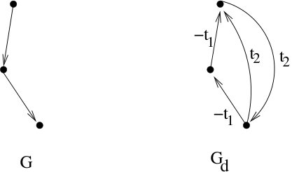 Figure 1
 Figure 2
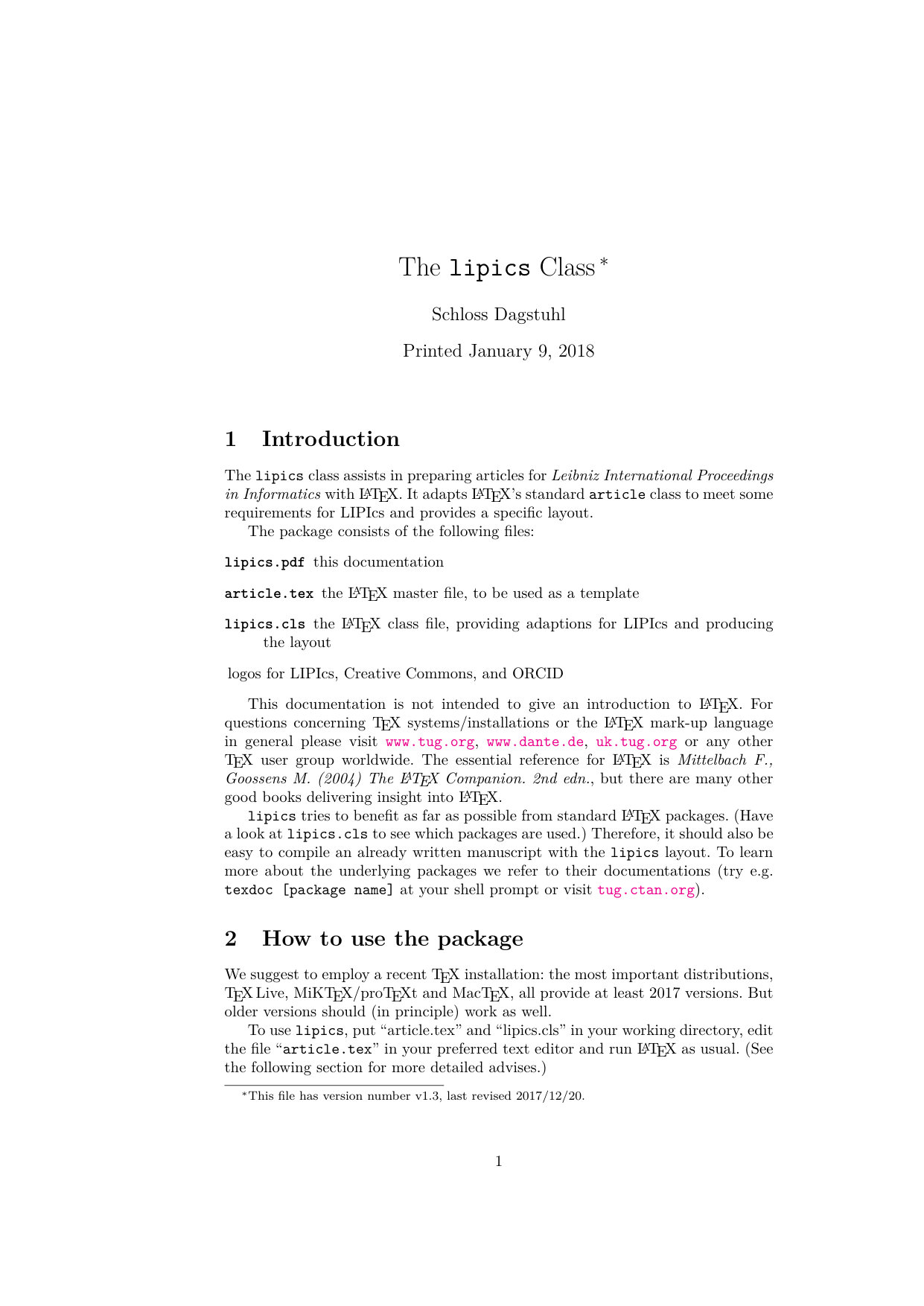 Figure 4
 Figure 5
 Figure 6
Peer Reviews
No public reviews on file for this paper yet. If you reviewed it on a platform where reviews are public (OpenReview, ICLR, NeurIPS, ICML), you can paste yours below so the community can read it here.
Videos
No videos yet. Explain this paper in a talk, walkthrough, or lecture? Add one.
Department of Mathematics, Indiana-Purdue University
[Fort Wayne, IN 46805, USA][email protected] Department of Computer Science, Colorado State University
[Fort Collins, CO 80523, USA][email protected] Department of Mathematics, Western Kentucky University
[Bowling Green, KY 42101][email protected] Department of Computer Science, Vanderbilt University
[Nashville, TN 37235, USA][email protected] Department of Computer Science, Colorado State University
[Fort Collins, CO 80523, USA][email protected]
\CopyrightPeter Hamburger and Ross M. McConnell and Attila Pór and Jeremy P. Spinrad and Zhisheng Xu
\EventEditorsIgor Potapov, Paul Spirakis, and James Worrell \EventNoEds3 \EventLongTitle43rd International Symposium on Mathematical Foundations of Computer Science (MFCS 2018) \EventShortTitleMFCS 2018 \EventAcronymMFCS \EventYear2018 \EventDateAugust 27–31, 2018 \EventLocationLiverpool, GB \EventLogo \SeriesVolume117 \ArticleNo69 \hideLIPIcs
Double Threshold Digraphs
Peter Hamburger
,
Ross M. McConnell
,
Attila Pór
,
Jeremy P. Spinrad
and
Zhisheng Xu
Abstract.
A semiorder is a model of preference relations where each element is associated with a utility value , and there is a threshold such that is preferred to iff . These are motivated by the notion that there is some uncertainty in the utility values we assign an object or that a subject may be unable to distinguish a preference between objects whose values are close. However, they fail to model the well-known phenomenon that preferences are not always transitive. Also, if we are uncertain of the utility values, it is not logical that preference is determined absolutely by a comparison of them with an exact threshold. We propose a new model in which there are two thresholds, and ; if the difference is less than , then is not preferred to ; if the difference is greater than then is preferred to ; if it is between and , then may or may not be preferred to . We call such a relation a double-threshold semiorder, and the corresponding directed graph a double-threshold digraph. Every directed acyclic graph is a double-threshold digraph; increasing bounds on give a nested hierarchy of subclasses of the directed acyclic graphs. In this paper we characterize the subclasses in terms of forbidden subgraphs, and give algorithms for finding an assignment of utility values that explains the relation in terms of a given or else produces a forbidden subgraph, and finding the minimum value of that is satisfiable for a given directed acyclic graph. We show that gives a useful measure of the complexity of a directed acyclic graph with respect to several optimization problems that are NP-hard on arbitrary directed acyclic graphs.
Key words and phrases:
posets, preference relations, approximation algorithms
1991 Mathematics Subject Classification:
Theory of computation Mathematics of computing Discrete Mathematics Graph theory
1. Introduction
A poset can be identified with a transitive digraph on its elements. The poset is a semiorder [12] if for some utility function we have if and only if . Semiorders were introduced as a possible mathematical model for preference in the social sciences. A first possible model for preference is the weak orders, in which each element is assigned a utility value, such that is preferred to iff the value of is greater than the value of . This was viewed as too restrictive; many preference relationships cannot be modeled by a weak order. Semi-orders were designed to model imprecision in the valuation function; we may be indifferent between elements not only if they have exactly the same values, but also if the difference between the values is smaller than some threshold. There is a great deal of literature on the subject of semiorders and preference; see the books [5, 14].
Our original motivation for defining double-threshold digraphs comes from an attempt to deal with an issue in mathematical psychology. Intuitively, it is natural to think that preference is transitive; if one prefers to and to , then one “should” prefer to . However, a variety of evidence exists showing that preferences are not always transitive. This has led to a great deal of discussion; for a summary of this issue, see [6]. Viewpoints range from the idea that the intuitive notion that preference is transitive are simply wrong and must be thrown away entirely to questioning whether what was being measured in the non-transitive findings was really a preference relation. Between these two views, there has been work on finding mathematical models that explain non-transitive preference; Fishburn [6] gives some possible models.
One approach to mathematical modeling is to try to give a reasonable model of extremely non-transitive preference; the famous cyclic voter’s paradoxes can be viewed as a model of preference which can allow not just non-transitivity, but also cycles.
Unlike these approaches, we generalize semi-orders to allow non-transitivity, but we require that the given set of preferences continue to be acyclic. In other words, we consider any preference relation represented by a directed acyclic graph (a dag). As in the case of semiorders, we assume that reported preferences are influenced by an underlying hidden utility function, which may be approximate, imperfectly known by a subject, or otherwise fail to capture all factors influencing a report of a preference.
One of our objectives is to obtain a measure of the departure of a given arbitrary acyclic set of pairwise preferences from a model where preferences are driven exclusively by an underlying hidden utility function, as well as derive an assignment of utility values that has the most explanatory power, in a sense that we define within a new model that we propose.
We propose a generalization of a semiorder, a double-threshold semiorder. We loosen the definition of a semiorder to a broader class of relations that are acyclic but not necessarily transitive, by allowing two thresholds and such that , and finding a valuation for each element . For two elements and , is not reported as a preference if , can freely be reported as a preference or not if , and is reported as a preference if . Let a satisfying utility function or a satisfying assignment of values for be a utility function that meets these constraints. This accommodates within the model the well-known phenomenon in the literature on perception that there can be a range of differences between the minimum difference that is sometimes perceived and the minimum difference that is perceived reliably.
When the relation of the double-threshold semiorder is modeled by a dag, it is called a double-threshold digraph. If a dag can be represented with thresholds , then it can be represented with any pair of thresholds such that , since a solution for can be turned into a solution for by rescaling all values by the factor . Therefore, for any pair of thresholds, the question of whether a particular dag can be represented with them depends on the ratio ; larger ratios allow representations of more dags.
Henceforth, given a digraph , let denote the number of vertices and the number of edges. When is understood, we may denote these as and . For a dag , let denote the minimum ratio of such that has a satisfying utility function for . When models a weak order, and for any has a satisfying utility function. For this trivial special case, which is easily recognized in linear time, we define to be 0, the lower bound on the satisfiable ratios , and call such a dag a degenerate dag. All other dags are nondegenerate.
When or the preference relation it models is understood, we denote simply by . For a dag that models a nondegenerate semiorder, ; higher values of provide a measure of the degree to which a given set of preferences depart from a semiorder. An acyclic preference relation is a -semiorder if it has a satisfying utility function for , that is, if . When such a preference relation is modeled as a digraph, we say the digraph is a double-threshold digraph. We show that for any nondegenerate dag , can be expressed as a ratio where and are integers such that (Theorem 2.4), allowing , , and the utility function to have small integer values. Also, for any dag, and is always satisfiable, so . An example of when the bound is tight is when is a directed path.
Thus, the classes of dags with bounded by different values give a nested hierarchy of dags, starting with weak orders and semiorders. For each class in the hierarchy, we give a characterization of the class in terms of a set of forbidden subgraphs for the class.
When has no satisfying utility function for , , we show how to return a forbidden subgraph as a certificate of this in time, where , and an time bound for finding (Theorem 18). The algorithm combines elements of the Bellman-Ford single-source shortest paths algorithm [1], Karp’s minimum mean cycle algorithm [10], and dynamic programming techniques based on a topological sort of a dag. For , a satisfying assignment, together with a forbidden subgraph for a smaller ratio, give a certificate that , and these take time to produce.
If is less than , must be transitive. The converse is not true: it is easy to show that the class of posets does not have bounded . Consider a chain in a poset and a vertex that is incomparable to the others; . Even though they are transitive, some posets are not good models of a preference relation that is based on an underlying utility function.
Although we show that bounding can make some NP-complete problems tractable, bounded-ratio double-threshold digraphs are in one sense enormously larger than semiorders. Semiorders correspond to digraphs that can be represented with ratio 1. These classes of digraphs both have implicit representations [15], implying that there are such digraphs on a set of labeled vertices. By contrast, every height 1 digraph can be represented with ratio : for each vertex , assign if is it a source or if it is a sink and make the thresholds . The number of such digraphs on labeled vertices, hence the number with ratio for any greater than or equal to 1, is .
The underlying undirected graph of a dag is the symmetric closure, that is, the undirected graph obtained by ignoring the orientations of the edges. In this paper, we say that a dag is connected if its underlying undirected graph is connected. Similarly, by a clique, coloring, independent set, or clique cover of a dag, we mean a clique, coloring, independent set or clique cover of the underlying undirected graph. Hardness results about these problems on undirected graphs also apply to dags, since every undirected graph is the underlying undirected graph of the dag obtained by assigning an acyclic orientation to ’s edges.
Finding a maximum independent set or clique in a dag takes polynomial time if the dag is transitive (a poset), hence if it is a semiorder, but for arbitrary dags, there is no polynomial-time approximation algorithm for finding a independent set or clique whose size is within a factor of of the largest unless P = NP [9]. However, for a connected dag , we give an algorithm for finding a maximum clique (Corollary 4.3), and an approximation algorithm that finds a clique whose size is within a desired factor of of that of a maximum clique in time (Corollary 4.5).
We show that finding a maximum independent set is still NP-hard when , but we give a polynomial-time approximation algorithm that produces an independent set whose size is within a factor of of the optimum (Theorem 4.7). We give approximation bounds of for minimum coloring and minimum clique cover (Theorems 4.9 and 4.10), which also have no polynomial algorithms for finding an approximation for arbitrary dags unless P = NP.
Thus, restricting attention to dags such that is bounded by a constant makes some otherwise NP-hard problems easy and gives rise to polynomial-time approximation algorithms that cannot exist in general unless P = NP. In each case, the time bound or the approximation bound is an increasing function of . This supports the view of as a measure of complexity of a dag. By contrast, for most similar attempts to measure complexity of a graph or digraph, the measurement is NP-hard to compute; examples include dimension of a poset, interval number, boxicity, and many others; see [15].
A concept similar to was given previously by Gimbel and Trenk in [7]. They developed a generalization of weak orders to partial orders that corresponds to the special case of a transitive dag. Not assuming transitivity requires us to use different algorithmic methods, but our bounds improve their bounds for their special case from and to . Most of their structural results are disjoint from ours because they are relevant to partial orders and their underlying undirected graphs, the comparability graphs.
2. Satisfying utility functions and forbidden subgraphs
We give the following formal definition:
Definition 2.1**.**
A dag is a double-threshold digraph if there exists an assignment of a real value to each vertex such that whenever is an edge, and whenever is not an edge, .
Whether the constraints can be satisfied can be formulated as the problem of finding a feasible solution to a linear program:
- •
for each such that is an edge;
- •
for each such that neither nor is an edge;
- •
for all .
The last constraint is added as a convenience; for any satisfying assignment, an arbitrary constant can be subtracted from all of the values to obtain a new satisfying assignment, so the constraint cannot affect the existence of a feasible solution.
This is a special case of a linear program, a system of difference constraints, where each constraint is an upper bound on the difference of two variables. This reduces to the problem of finding the weight of a least-weight path ending at each vertex in a digraph derived from the constraints, as described in [1], where there is a satisfying assignment if and only if the digraph of the reduction has no negative-weight cycle. Applying the reduction to the problem of determining whether there is a satisfying utility function on yields a digraph , where (see Figure 1). has an edge of weight for each edge of , and edges and of weight for each pair such that neither of and is an edge of . A negative cycle in proves that the system is not satisfiable; otherwise, for each , assigning to be the minimum weight of any path ending at gives a satisfying assignment for .
The single-source least-weight paths problem where some weights are negative can be solved in time, but has edges, so a direct application of this approach takes time to find a satisfying assignment or produce a negative-weight cycle in . We derive tighter bounds below.
In terms of , a negative cycle of translates to a forbidden subgraph characterization of double-threshold digraphs:
Definition 2.2**.**
Let be a hop in if neither nor is an edge of . Let a forcing cycle be a simple cycle such that such that for each consecutive pair (indices mod ), the pair is either a directed edge of or a hop. Let the ratio of the forcing cycle be the ratio of the number of edges to the number of hops.
Theorem 2.3**.**
For a nondegenerate dag , the minimum satisfiable ratio is equal to the maximum ratio of a forcing cycle in .
One consequence of the theorem is that when is a nondegenerate dag, a satisfying assignment of values for thresholds , together with a forcing cycle with ratio equal to gives a certificate that , as illustrated in Figure 2.
Theorem 2.4**.**
For every nondegenerate dag , can be expressed as a ratio of integers such that .
Proof 2.5**.**
This follows from the fact that and is the ratio of the number of edges to the number of hops on a forcing cycle.
Aside from showing that optimum values of and can be expressed as small integers, the theorem gives an immediate bound for finding . This is because it implies that the number of possible values that can take on is , and that these can be generated and sorted in time. A binary search on this list, spending time at each probe to determine whether is an double-threshold digraph, as described above, can then be used to find . Once is known, a satisfying assignment of utility values for , together with a forcing cycle with forcing ratio equal to gives a certificate that the claimed value of is correct. We improve these bounds to in section 5.
3. -clique extendable orderings
In the book [15], Spinrad introduced the class of -clique extendable orderings of the vertices of graphs, which we explain below. Finding whether a graph has a 2-clique extendable ordering takes polynomial time, but no polynomial time bounds are known for . However, we show in the next section that a topological sort of a nondegenerate dag is a -clique extendable ordering for , and develop several applications of this result to optimization problems. In this section, we give the details and analysis of the time bound of an algorithm suggested in [15] for finding a maximum clique, given a -clique extendable ordering.
Two sets overlap if they intersect and neither is a subset of the other. Let be an ordering of the vertices of a graph, . For let us say that ends with if the elements of are the last elements of in , that is, if no element of occurs after an element of . begins with if ends with in .
Definition 3.1**.**
An ordering of vertices of a graph is -clique extendable ordering of if, whenever and are two overlapping cliques of size , , and begins with and ends with in , then and are adjacent and is a clique.
This is a generalization of transitivity, since a dag is transitive if and only if its topological sorts are two-clique extendable orderings, hence a graph is a comparability graph if and only if it has a two-clique extendable orderings. In [15], it is shown that three-clique extendable orderings arise naturally in connection with visibility graphs, and that it takes polynomial time to find a maximum clique in a graph, given a three-clique extendable ordering. A polynomial-time generalization for -clique extendable orderings is implied; we give details and a time bound next.
Lemma 3.2**.**
If is a -clique extendable ordering of a graph and and are overlapping cliques of any size greater than or equal to , such that and begins with and ends with in , then is a clique.
Proof 3.3**.**
It suffices to show that every element of is adjacent to every element of . Let be an arbitrary element of , be an arbitrary element of , and be any elements of . Then and are two -cliques and, by the definition of a -clique extendable ordering, their union is a clique, and and are adjacent.
Corollary 3.4**.**
If is a -clique extendable ordering of a graph , is a -clique ending with and is a largest clique of ending with the -clique , then is a largest clique of ending with .
Proof 3.5**.**
For any clique ending with , is a clique ending with . , which is a clique by Lemma 3.2.
Corollary 3.4 is the basis of the recurrence for a dynamic programming algorithm for finding a maximum clique of , given a -clique extendable ordering. We enumerate all -cliques and then label each -clique with the maximum size of a clique that ends with . If is the left-to-right ordering of a -clique in the ordering, then its label is one plus the maximum of the labels of cliques of the form . The size of the maximum clique of is the maximum of the labels. Details and the proof of the following resulting time bound is given in the appendix.
Theorem 3.6**.**
Given a -clique extendable ordering of a graph , a maximum clique can be found in time.
It is easy to see that when the vertices of have positive weights, the problem of finding a maximum weighted clique can be solved in the same time bound, using a trivial variant of Corollary 3.4.
4. Optimization problems on dags with bounded values
We now show that restricting attention to dags such that is bounded by a constant makes some otherwise NP-hard problems easy or gives rise to polynomial-time approximation algorithms that cannot exist for the class of all dags unless P = NP. The NP-hard problems we consider can be trivially solved in linear time on degenerate dags, so we focus on nondegenerate dags.
Theorem 4.1**.**
Let be a nondegenerate dag and . A topological sort of is a -clique extendable ordering.
Proof 4.2**.**
Let be a topological sort, and let be a satisfying utility function for such that . Let and be the left-to-right orderings of two -cliques and . Then is a directed path in , hence , is an edge and is a clique.
Corollary 4.3**.**
It takes time to find a maximum clique in a connected nondegenerate dag .
Proof 4.4**.**
To avoid an additive term, run the dynamic programming algorithm on a topological sort under the assumption that it is a 2-clique extendable ordering in time by Theorem 3.6, and return the result if it is a clique. Otherwise, do the same under the assumption that it is a 3-clique extendable ordering, in time. If a max clique has not yet been returned, then by Theorem 4.1, so compute in time, which is now subsumed by the bound we want to show. A topological sort is a extendable ordering by Theorem 4.1, so it takes time to find a maximum clique by Theorem 3.6.
Even if is bounded by a moderately large constant, this bound could be prohibitive in practice, but it also gives an approximation algorithm that allows a tradeoff between time and approximation factor:
Corollary 4.5**.**
Given a connected nondegenerate dag and integer such that , a clique whose size is within a factor of of the size of a maximum clique can be found in time.
Proof 4.6**.**
Let be the result of removing the edges and . A satisfying function for and thresholds is also a satisfying function for and thresholds , so . Applying Theorems 3.6 and 4.1, we get a maximum clique of in time. A maximum clique of induces a directed path in , and is a clique of , so the size of a maximum clique in is within a factor of of the size of a maximum clique in .
If , a maximum independent set in can be obtained in polynomial time, since is transitive [8]. However, even when , the problem of determining whether has an independent set of size is NP-complete. This is seen as follows. It is NP-complete to decide whether a 3-colorable graph has an independent set of a given size , even when the 3-coloring is given [11]. Given such a graph , , and three-coloring, let , , and be the three color classes. Every edge has endpoints in two of the classes; orient from the endpoint in the class with the smaller subscript to the endpoint in the class with the larger subscript. Doing this for all edges results in a dag such that , since, for each vertex , if , assigning gives a satisfying assignment of utility values for and . There is an independent set of size in if and only if there is one in .
Theorem 4.7**.**
For in the class of dags where , there is a polynomial -approximation algorithm for the problem of finding a maximum independent set in .
Proof 4.8**.**
Find a satisfying assignment of utility values for such that , then find an interval of the form such that the size of the set whose values are in the interval is maximized. is an independent set, since no pair of them has values that differ by . Return these vertices as an independent set.
For the approximation bound, let be a maximum independent set. The values of lie in an interval of the form , which is a subset of the union , of intervals of the form , hence .
Proofs of the following make similar use of the availability of satisfying values are given in the appendix.
Theorem 4.9**.**
For in the class of dags where , there is a polynomial -approximation algorithm for the problem of finding a minimum coloring of .
Theorem 4.10**.**
For in the class of dags where , there is a polynomial -approximation algorithm for the problem of finding a minimum clique cover of .
5. bounds for finding satisfying utility
functions, , and certificates
In this section, we first show how to find a satisfying assignment of utility values for given thresholds , in time, where . We then show how to find in time. By solving the second problem to find , then selecting such that and solving the first, we get the certificates for , that is, a satisfying assignment and a cycle such that the ratio of edges to hops is , which comes from a zero-weight cycle in .
For both of these problems, we use the following. When is an arbitrary digraph where each vertex has a weight and each edge has a weight , it takes time to find is an edge of for each vertex of . Let us call this the general relaxation procedure. In the special case where is a dag, it takes time to find , where is the minimum weight of any path from to and = 0. This can be used to solve the single-source shortest paths problem on a connected dag in time [1]. Let us call this the dag variant of the relaxation procedure.
In a digraph with edge weights, let the length of a walk be the number of occurrences of edges on the walk and its weight be the sum of weights of occurrences of edges. If an edge occurs times on the walk, it contributes to the length, and if its weight is , it contributes to the weight and to the number of (occurrences of) edges of weight on the walk.
5.1. Finding a satisfying utility function or a forbidden subgraph for
.
The Bellman-Ford algorithm is a dynamic programming algorithm that works as follows on a connected digraph where a vertex has been added that has an edge of weight zero to all other vertices. Let be the minimum weight of any walk from to that has at most edges. is just the minimum weight of any walk of length at most in ending at ; henceforth we omit from the discussion. for all . During the “ pass” the algorithm computes as . This is just an instance of the general relaxation procedure where and the loop is considered to be an edge of weight 0 for each . If there is no negative cycle, there is always a path ending at that is a minimum-weight walk ending at , so gives the minimum weight of any path ending at . If there is a negative cycle, this is detected when for some , indicating a walk of length of smaller weight of any path, which must have a negative cycle on it. By annotating the dynamic programming entries with suitable pointers, it is possible to find such a cycle within the same bound. The passes to compute for all each take time, for a total of time.
To exploit the structure of to improve the running time, we let denote the minimum weight of any path that has at most edges of weight , rather than at most edges in total. We use the elements , rather than the elements of , as the elements of the dynamic programming table. Let us call this reindexing the dynamic programming table. We obtain by assigning and running the dag variant of the relaxation procedure on the edges of weight , since they are acyclic. For pass such that , any improvements obtained by allowing an edge of weight are computed with the general relaxation procedure, where loops are considered to be edges of weight 0, and, after this, any additional improvements obtained by appending additional edges of weight are computed by the dag variant of the relaxation procedure.
Because every vertex has a walk of length and weight 0 ending at it, for . Therefore, for , if , the ratio of edges of weight to edges of weight is greater than . Any such walk must have more than edges of weight , hence length greater than . Therefore, if there is no negative cycle in , for , , and a negative cycle occurs if for this and some . A negative cycle can be found by the standard technique of annotating the results of the relaxation operations with pointers to earlier results. The advantage of reindexing the table is that the algorithm now takes passes instead of of them.
To get the bound, it remains to show how to perform each pass in time. The bottleneck is evaluating is an edge of weight for the general relaxation step. Since all of the edges have the same weight, we rewrite this as where minimizes for all such that . To evaluate this, we just have to find . At the beginning of the pass, we radix sort the vertices in ascending order of , giving list . To compute , we mark the vertices that have an edge to , then traverse until we find as the first unmarked vertex we encounter, then unmark the vertices that have edges to . This takes time proportional to the in-degree of , hence time for all vertices in the pass.
5.2. Finding
To find , we use the fact that that if , the corresponding weighting of will give it a zero-weight cycle in , which gives a forcing cycle of ratio in as a certificate.
For arbitrary , let the mean weight of a directed cycle or path of length at least one in be the weight of the cycle divided by the number of edges. The minimum mean weight of a cycle is the minimum cycle mean. Subtracting a constant from the weight of all edges in subtracts from the mean weight of every cycle and path of length at least one. For arbitrary and , weighting in accordance with in place of has the same effect of subtracting from the weights of all edges. Thus, for arbitrary , if is the minimum cycle mean of the corresponding weighting of , then . Finding reduces to finding the minimum cycle mean in the weighting of obtained from an arbitrarily assigned .
In a digraph with edge weights, let be the minimum weight of any walk of length exactly ending at . In [10], Karp showed the following:
Theorem 5.1**.**
*The minimum cycle mean of a digraph with edge weights is
.*
Karp actually shows this when an arbitrary vertex is selected and is defined to be the minimum weight of all walks of length from to , but if it is true for walks beginning at an arbitrary vertex , then it is true when is allowed to vary over all vertices of . Omitting from consideration in this way in his proof gives a direct proof of this variant of his theorem. He reduces the problem to the special case where is strongly connected by working on each strongly-connected component separately, but the only purpose of this in his proof is to ensure that there is a path from to all other vertices, and this is unnecessary when is allowed to vary over all vertices.
can be computed by a variant of Bellman-Ford, by using the recurrence in place of . The only difference from the algorithm of Section 5.1 is that loops of the form are not considered to be edges. Computing for all takes passes, each of which applies the general relaxation operation, for a total of time.
An obstacle to an bound that we did not have in Section 5.1 is that in Theorem 5.1, computing for requires computations, which is not .
We again reindex the dynamic programming table (Section 5.1), letting denote the minimum-weight walk ending at in that has exactly edges of weight . We compute the values in passes, computing for each during pass . As in Section 5.1, each pass takes takes time; the only change is that in the general relaxation step, loops are not considered to be edges. We claim that passes suffice, but a new difficulty is knowing when to stop, since, unlike of the Section 5.1, is not known in advance.
A walk with edges of weight and weight has edges of weight , so it must have edges of weight . Its length, , can be computed as in time.
Let a term be term of interest if , that is, if it corresponds to a walk of interest of length . We use the following reindexed variant of Karp’s theorem, which says that it suffices to compute an inner maximum over a smaller set, and only for terms of interest. The proof is the one Karp gives, reindexed, and omitting reference to a start vertex by allowing the start vertex to vary over all vertices. For completeness, we give the modified proof in the appendix.
Theorem 5.2**.**
*In , the minimum mean weight of a cycle is equal to
*
The solution is given as Algorithm 1. During the pass, the algorithm computes for all . Before proceeding to the next pass, it updates a partial computation of the expression of Theorem 5.2, computing for each the terms of interest that has been computed during the pass, and keeping track of the minimum of these computations so far. Let a term of interest be critical if the minimum cycle mean is equal to . The strategy of the algorithm is to return the minimum it has found so far once it detects that a critical term has been evaluated.
Let a critical walk be a walk of length giving rise to a critical term.
Lemma 5.3**.**
In , the mean weight of a critical walk is less than or equal to the minimum cycle mean.
The proof is given in the appendix.
Theorem 5.4**.**
Given a nondegenerate dag , it takes time to find .
Proof 5.5**.**
The basis of this is Algorithm 1. For a term of interest, , the mean weight of the corresponding walk is , which is an increasing function of . Thus, once this exceeds the minimum value, , found so far a critical term has been found and is already reflected in the value of . Thus, Algorithm 1 returns the minimum cycle mean.
The minimum cycle mean is the ratio of edges of weight to edges of weight on a cycle of minimum mean. This must also be true for a critical walk, by Lemma 5.3. This ratio for the walks of interest in pass is , so the algorithm halts before the first pass such that , and . Thus, Algorithm 1 halts after passes.
Using the approach of Section 5.1, the operations in a pass take time except for evaluating for terms of interest. For any vertex , is a term of interest for at most one value of . Therefore, the cost of evaluating for terms of interests is bounded by the total number of dynamic programming table entries for and computed by the algorithm, which is the number of them computed in each pass times passes. This is .
6. Appendix
Theorem 3.6: Given a -clique extendable ordering of a graph , a maximum clique can be found in time.
Proof 6.1**.**
Let be the -clique extendable ordering. There are cliques in a connected graph with edges, and they can be enumerated in time [2]. If there are no -cliques, a maximum clique can be found in time by applying this algorithm to find all -cliques for .
Otherwise, we denote each -clique with a tuple where are the elements of the clique and in the -clique extendable ordering. We order the cliques lexicographically by the reverse of its tuple (cliques sharing the last members are consecutive in the list). The lexicographic sort takes time, since there are of them. This list serves as the dynamic programming table, which has one entry for each -clique. In addition we create a block, identified as for each nonempty block of cliques that share as their rightmost elements; they are consecutive in the dynamic programming table. This block is relevant to each -clique of the form . We precompute a pointer from each clique to its relevant block by lexicographically sorting the cliques by their first elements in reverse order. This order is the order of their blocks in the table, so traversing this list and the table concurrently allows assignment of the pointers from cliques to their relevant blocks time.
The dynamic programming labels each -clique with the size of the maximum clique of ending with its elements, and each block with the maximum of the labels of cliques in the block. This can be done in lexicographic order: when the last clique in a block has been labeled, the block is labeled with the maximum of the labels of the cliques in the block, and when clique is reached, its label is one plus the maximum of the labels in its relevant block , which is already labeled. Traversing the table performing these operations, using the precomputed pointers to blocks, takes time.
The maximum label of any -clique tells the size of a maximum clique in the graph. Let be a -clique with maximum label. To reconstruct the maximum clique of the graph, note that the last elements of this clique are . Find the remaining elements, as follows: recursively find all but the last elements of the largest clique ending on a -clique in ’s relevant block, which is empty if has no relevant block, and add to this result.
Theorem 4.9: For in the class of dags where , there is a polynomial -approximation algorithm for the problem of finding a minimum coloring of .
Proof 6.2**.**
Given a nondegenerate dag , find a satisfying assignment of utility values for such that .
Let be the lowest value assigned by the algorithm to any of the vertices, and let be the highest. Partition the interval into buckets of the form for . For each bucket, return the vertices whose values lie in each bucket as the color classes.
Let be a vertex such that . In an optimum coloring, , removal of the color class containing removes a subset of the set of vertices in the first buckets since it is an independent set. Removal of the color classes of the returned coloring that correspond to the first buckets advances the minimum value among the remaining vertices by . Removal of the of the color class in an optimum coloring containing advances it by at most that much. By induction on the number of vertices, we may assume that the number of remaining color classes of the returned coloring is at most times the number of color classes in the remainder of . Thus, for every color class in an optimum coloring, there are at most in the coloring returned by the algorithm.
Theorem 4.10: For in the class of dags where , there is a polynomial -approximation algorithm for the problem of finding a minimum clique cover of .
Proof 6.3**.**
Given a nondegenerate dag , find a satisfying assignment of utility values for such that .
Let be a value such that contains the values of a maximum number of vertices. Select from among the vertices whose value lie in . Select so that for , minimizes over all vertices such that . Select such that for , maximizes over all vertices such that . Let be the union of these two sets. Because the pairwise differences in values are greater than , is a clique. Let this be one of the cliques in the clique cover. Remove it from the set of vertices, and recurse on the remaining vertices to get the remaining cliques of the cover.
To see that this has an approximation ratio of at most , let be the set of vertices whose values are in . Each clique of the clique cover returned by the algorithm removes one vertex from . In a minimum clique cover, each pair of vertices must have values that differ by at least . Thus, no clique can contain more than vertices from . The clique cover returned by the algorithm has at most times the number of cliques as a minimum clique cover.
Lemma 5.3: In , the mean weight of a critical walk is less than or equal to the minimum cycle mean.
Proof 6.4**.**
Let be assigned arbitrarily. Since we may apply the result separately to each strongly connected component of , we may assume that is strongly connected. Let be the result of subtracting from every edge weight in . The mean weight of , hence its total weight, is 0 in . Since they all have the same length , the paths of interest in are the same as they are in .
Out of all paths ending at a vertex on , let be one of minimum weight in , let be its weight in , and let be the last vertex of . Let be the walk of length obtained by walking round and round , starting at , let be the last vertex of , and let be the walk of length obtained by concatenating and . Let be the first vertex of .
In , the weight of is equal to the minimum weight of a walk of any length ending at , which is seen as follows. Suppose there is a walk of weight , ending at . Let be the weight of the portion of directed from to , and let be the weight of the portion of directed from to . Since has weight 0, . Appending to the portion of from to gives a walk ending at of weight , and, since has weight 0, this is just . Removing any cycles from this walk, we get a path of weight , contradicting that is a path of minimum weight to .
Thus, is a walk of interest in , hence in . In , since there is a walk of length 0 and weight [math] ending at , so the weight of in , hence its mean weight in is at most the minimum cycle mean of 0 in in . Its mean weight in is at most the minimum cycle mean of .
Since the edges of weight are acyclic there is at least one edge of weight on . Since has length and is the only cycle on it, makes at least one complete revolution of , and the weight of is for some . Therefore, and is a term of interest, and the mean weight of its walk of interest is the minimum cycle mean.
Theorem 5.2: *In , the minimum mean weight of a cycle is equal to
*
The proof requires a lemma:
Lemma: If the minimum cycle mean is zero, then
.
Proof 6.5**.**
Suppose . Because there are no negative cycles, there is a minimum-weight walk ending at whose length is less than . Let its weight be . . Also, , so , and .
Equality holds if and only if . We complete the proof by showing that there exists such that there exists where and . Let be a cycle of weight zero and let be a vertex on . Let be a path of weight ending at . Then , followed by any number of repetitions of , is also a minimum-weight walk to its endpoint. After sufficiently many repetitions of , such an initial part of length will occur; let its endpoint be . Then for some , and . Choosing , the proof is complete.
Proof of Theorem 5.2. Reducing the weight of each edge weight by a constant reduces the minimum cycle mean by , and is reduced by . If , is reduced by , and is reduced by . The minimum cycle mean and this expression are affected equally. Choosing to be the minimum cycle mean and then applying the lemma, we complete the proof.
The reference list from the paper itself. Each links out to its DOI / PubMed record.
- 1[1] Thomas H. Cormen, Charles E. Leiserson, Ronald L. Rivest, Clifford Stein, Introduction to Algorithms, MIT 2009
- 2[2] Norishige Chiba, Takao Nishizeki, Arboricity and Subgraph Listing Algorithms, SIAM J. Comput. 14 (1985), 210–223.
- 3[3] Peter C. Fishburn, Intransitive Indifference with Unequal Indifference Intervals, J. Math. Psych. 7 (1970), 144–149.
- 4[4] Peter C. Fishburn, Interval Representation for Interval Orders and Semiorders, J. Math. Psych. 10 (1973), 91–105.
- 5[5] Peter C. Fishburn, Interval Orders and Interval Graphs: Study of Partially Ordered Sets, Wiley (1985)
- 6[6] Peter C. Fishburn, Nontransitive Preferences in Decision Theory, Journal of Risk and Uncertainty 4 (1991), 113–134
- 7[7] John G. Gimbel, Ann N. Trenk, On the Weakness of an Ordered Set, SIAM J. Discrete Math, 11 (1998), 655–663.
- 8[8] Fanica Gavril, Maximum Weight Independent Sets and Cliques in Intersection Graphs of Filaments, Information Processing Letters 11 (2000), 181–188.