Hyperbolic graphs: critical regularity and box dimension
Lorenzo J. D\'iaz, Katrin Gelfert, Maik Gr\"oger, Tobias J\"ager

TL;DR
This paper investigates the fractal and regularity properties of invariant graphs in hyperbolic skew product systems, providing formulas for their box dimension and analyzing different dynamical scenarios.
Contribution
It introduces a formula for the box dimension of invariant graphs in hyperbolic systems and characterizes their regularity based on the base dynamics and the presence of fibered blenders.
Findings
Derived a formula for box dimension using pressure functions.
Identified three dynamical scenarios affecting regularity and dimension.
Established the role of fibered blenders in dimension analysis.
Abstract
We study fractal properties of invariant graphs of hyperbolic and partially hyperbolic skew product diffeomorphisms in dimension three. We describe the critical (either Lipschitz or at all scales H\"older continuous) regularity of such graphs. We provide a formula for their box dimension given in terms of appropriate pressure functions. We distinguish three scenarios according to the base dynamics: Anosov, one-dimensional attractor, or Cantor set. A key ingredient for the dimension arguments in the latter case will be the presence of a so-called fibered blender.
Click any figure to enlarge with its caption.
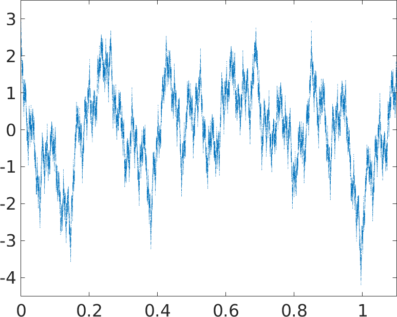 Figure 1
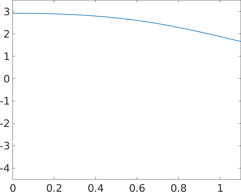 Figure 2
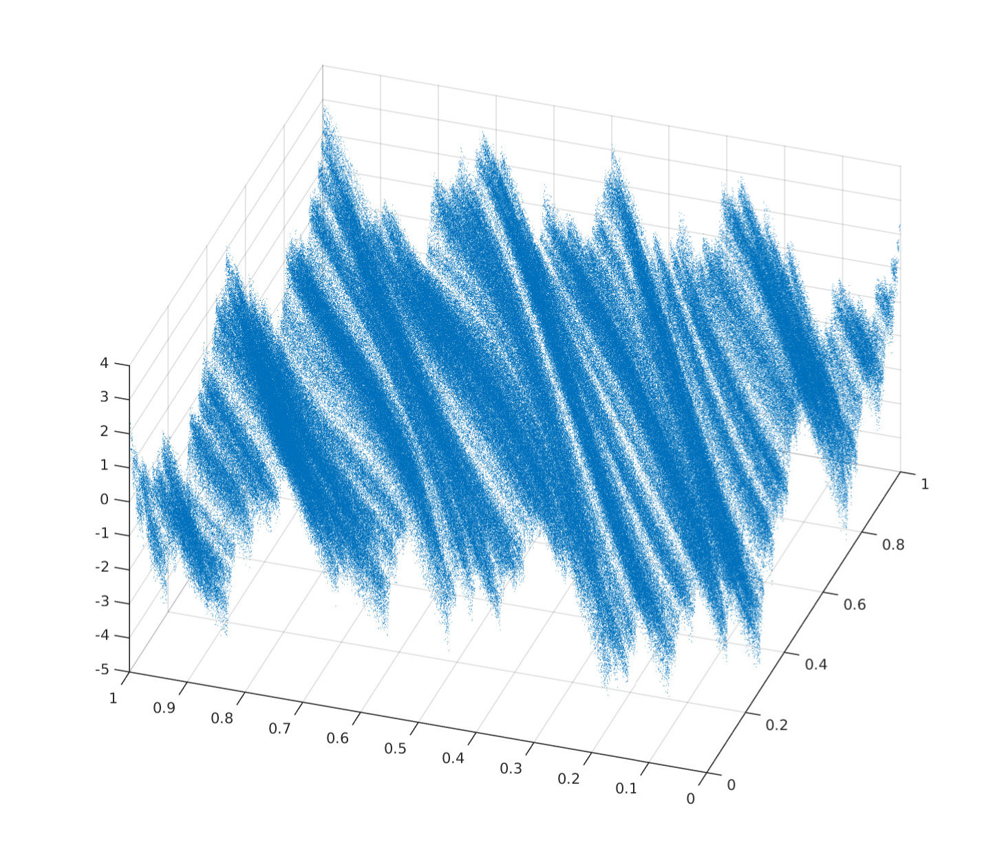 Figure 3
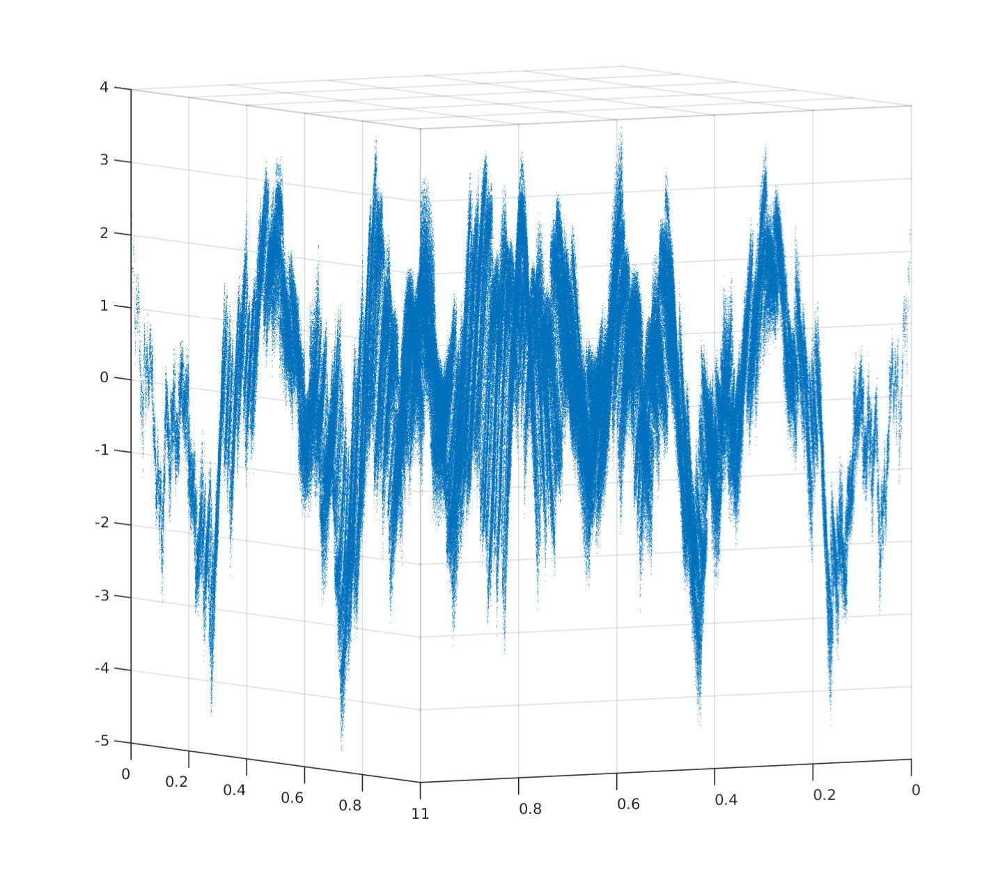 Figure 4
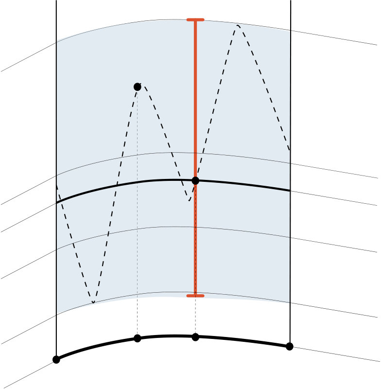 Figure 5
 Figure 6
 Figure 7
 Figure 8
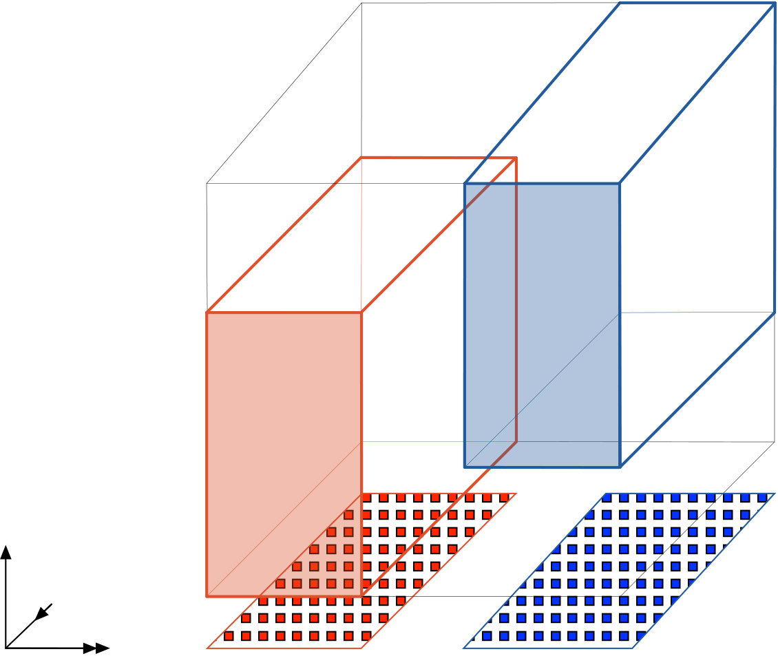 Figure 9
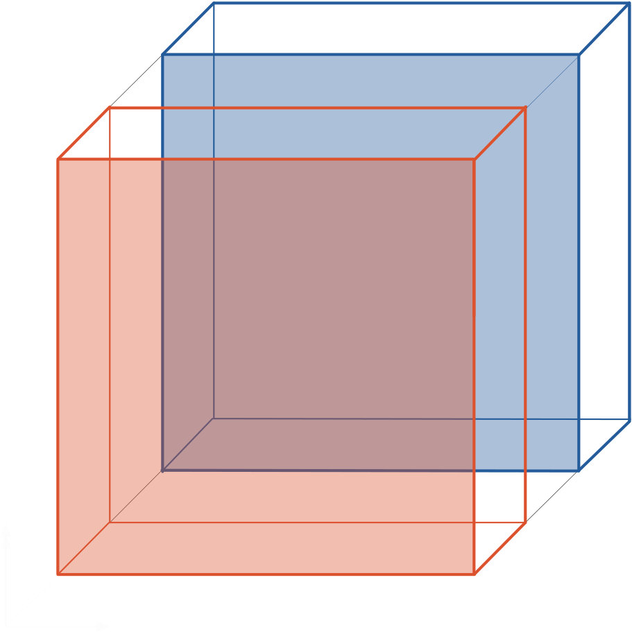 Figure 10
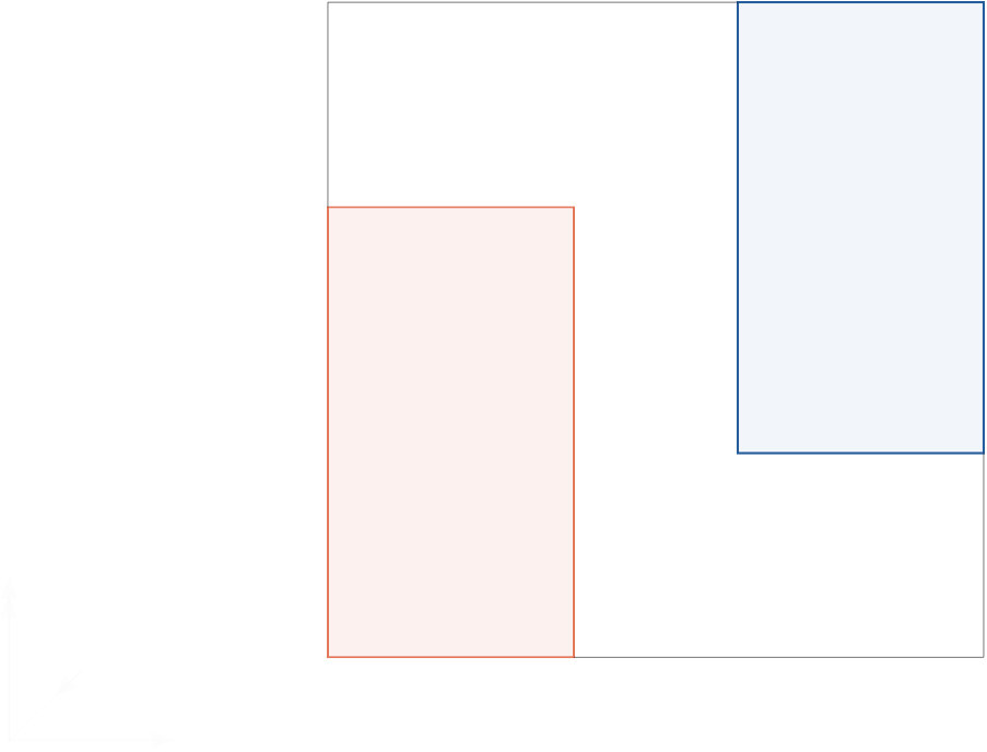 Figure 11
 Figure 12
 Figure 13
 Figure 14
 Figure 15
 Figure 16
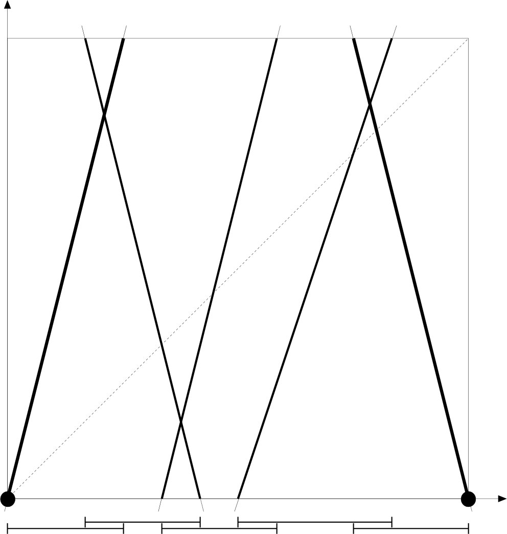 Figure 17
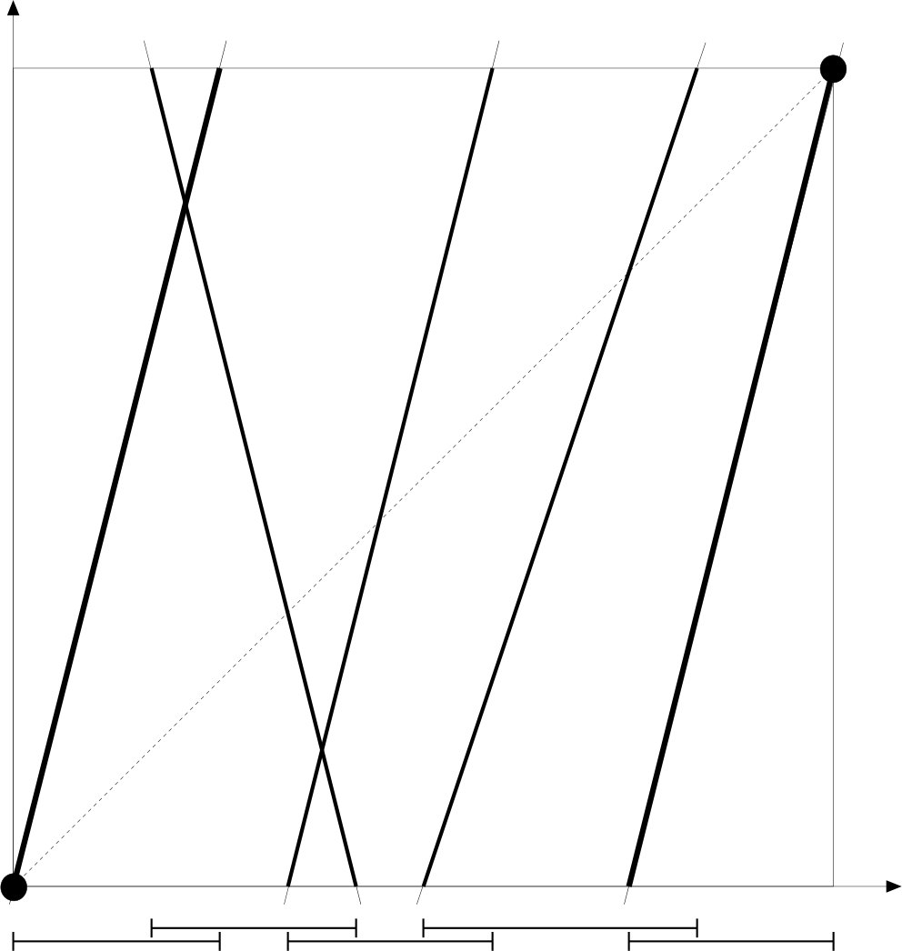 Figure 18
 Figure 19
 Figure 20
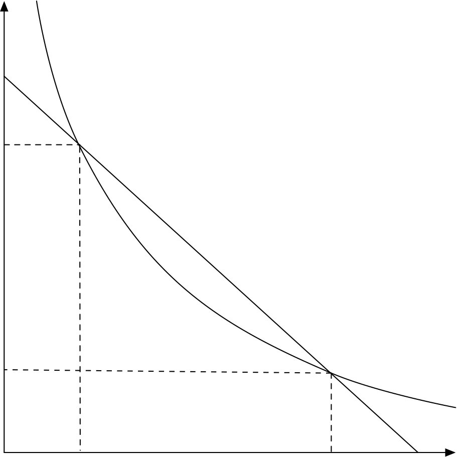 Figure 21
Peer Reviews
No public reviews on file for this paper yet. If you reviewed it on a platform where reviews are public (OpenReview, ICLR, NeurIPS, ICML), you can paste yours below so the community can read it here.
Videos
No videos yet. Explain this paper in a talk, walkthrough, or lecture? Add one.
Taxonomy
TopicsMathematical Dynamics and Fractals · Chaos control and synchronization · Quantum chaos and dynamical systems
Hyperbolic graphs:
critical regularity and box dimension
,
L. J. Díaz
Departamento de Matemática PUC-Rio, Marquês de São Vicente 225, Gávea, Rio de Janeiro 22451-900, Brazil
,
K. Gelfert
Instituto de Matemática Universidade Federal do Rio de Janeiro, Av. Athos da Silveira Ramos 149, Cidade Universitária - Ilha do Fundão, Rio de Janeiro 21945-909, Brazil
,
M. Gröger
Friedrich-Schiller-University Jena, Institute of Mathematics, Ernst-Abbe-Platz 2, 07743 Jena, Germany
and
T. Jäger
Friedrich-Schiller-University Jena, Institute of Mathematics, Ernst-Abbe-Platz 2, 07743 Jena, Germany
Abstract.
We study fractal properties of invariant graphs of hyperbolic and partially hyperbolic skew product diffeomorphisms in dimension three. We describe the critical (either Lipschitz or at all scales Hölder continuous) regularity of such graphs. We provide a formula for their box dimension given in terms of appropriate pressure functions. We distinguish three scenarios according to the base dynamics: Anosov, one-dimensional attractor, or Cantor set. A key ingredient for the dimension arguments in the latter case will be the presence of a so-called fibered blender.
Key words and phrases:
box dimension, fibered blender, invariant graph, hyperbolicity, skew product, topological pressure
2000 Mathematics Subject Classification:
37C45, 37D20, 37D35, 37D30
This research has been supported, in part, by CNE-FaperjE/26/202.977/2015 and CNPq research grants 302879/2015-3 and 302880/2015-1 and Universal 474406/2013-0 and 474211/2013-4 (Brazil) and EU Marie-Curie IRSES Brazilian-European partnership in Dynamical Systems FP7-PEOPLE-2012-IRSES 318999 BREUDS and DFG Emmy-Noether grant Ja 1721/2-1 and DFG Heisenberg grant Oe 538/6-1. This project is also part of the activities of the Scientific Network “Skew product dynamics and multifractal analysis” (DFG grant Oe 538/3-1). Further, LD and KG thank ICERM (USA) and CMUP (Portugal) for their hospitality and financial support.
1. Introduction
We study regularity properties and box dimension of fractal graphs appearing as attractors, repellers, or saddle-sets in skew product dynamics.
Our motivation is two-fold. First, there is an intrinsic interest in the fractal properties of such graphs, which is best exemplified by the well-known and paradigmatic examples of Weierstrass functions. Based on dynamical methods, recent advances have allowed to obtain a detailed understanding of their fractal structure including their Hausdorff dimension (thus solving a long-standing conjecture) [1, 24, 40].
Second, there is a general motivation for these endeavors. The investigation of fractal attractors, repellers, horseshoes, and other types of hyperbolic sets has been a major driving force for many important developments in ergodic theory and its interfaces with mathematical physics and fractal geometry (see, for instance, [26, 32, 14] for more information). Thereby, the situation is fairly well understood for two-dimensional hyperbolic systems (see [28, 44, 31] and Theorem 1.1 below), which is essentially a conformal setting and comparable to the study of conformal repellers (see [36]). However, extending the theory to higher-dimensional and genuinely nonconformal situations is well known to be difficult, and there exist only few and specific results in this direction (see, for example, [22, 12, 41, 18] and more details in Remark 1.3). Amongst the different phenomena that complicate matters are:
- •
The possible loss of equality between Hausdorff and box dimensions,
- •
both dimensions may not vary continuously with the dynamics.
A natural, and quite common, approach to proceed is to study gradually more complex (e.g. higher-dimensional) systems. We proceed by studying graphs in three-dimensional skew product systems
[TABLE]
with hyperbolic surface diffeomorphisms, or their restrictions to basic pieces , in the base, building on previous results in [22, 3, 15]. Summarizing our main results, except in a nongeneric case when the graph is Lipschitz, its box dimension is given by , where is the dimension of stable slices of and where is determined as the unique solution of the pressure equation
[TABLE]
Here are appropriately defined geometric potentials taking into account the expansion rates in the fiber center unstable and the strong unstable directions, respectively. The above formula will be established in three scenarios (Anosov in the base, one-dimensional attractors in the base, and fibered blenders). These results can be viewed as a natural step to address the corresponding technical and conceptual problems in a nontrivial, but still accessible setting. Thereby, we focus on the box dimension as the most accessible quantity in a first instance. Although eventually our approach could be instrumental for describing finer fractal properties like the Hausdorff dimension or carrying out a multifractal analysis as well, which is beyond the purposes of this paper.
1.1. Previous results on basic sets of surface diffeomorphisms
Before stating our first main result, let us provide more details on what is known in the two-dimensional case. Let be a surface diffeomorphism. Recall that a set is basic if it is compact, invariant, locally maximal in the sense that there is an open neighborhood of such that , topologically mixing, and hyperbolic in the sense that there exist a -invariant splitting and numbers such that for every
[TABLE]
(up to an equivalent change of metric), where and denote the derivative of at in the stable and unstable directions, respectively. Further, recall that basic sets have a (local) product structure, that is, they can locally be described as products of representative stable and unstable slices, given by the intersection of with the local stable and unstable manifolds, respectively (see [23]). In dimension two, their Hausdorff and box dimensions coincide and are given by the following classical Bowen-Ruelle type formula which is a compilation of results in [28, 44, 31]. Consider for a basic set the functions (also called potentials)
[TABLE]
We denote by the topological pressure of a potential (with respect to ) (see Section 2.1 for more details). Further, and denote the local stable and the local unstable manifold of (with respect to ), respectively (see Section 4.1 for more details). Last, denote by the Hausdorff dimension and by the box dimension of a totally bounded subset in a metric space. In general, we have . We recall the definition of box dimension and some properties in Section 2.2; further information can be found in [13].
Theorem 1.1** ([28, 44, 31]).**
Consider a basic set of a surface diffeomorphism . Let and be the unique real numbers for which
[TABLE]
Then for every we have
[TABLE]
where stands either for or . Moreover, we have
[TABLE]
Remark 1.2**.**
Formulas (1.3) were derived for the Hausdorff dimension in [28]. That Hausdorff and box dimension coincide was shown in [44] for diffeomorphisms and in [31] as stated above (in fact, [31] assumes only). To infer that the Hausdorff dimension of the (local) product is the sum of the dimensions of the intersections in (1.3) is conditioned to the fact that Hausdorff and box dimension coincide (see [13]). It requires the regularity of the stable/unstable holonomies, too. Yet, for hyperbolic surface diffeomorphisms these holonomies are always bi-Lipschitz. In [31], the authors also establish the continuous dependence of the dimensions on the diffeomorphism.
Remark 1.3**.**
In general, as already mentioned, in higher dimensions the above statements do not remain valid. For example, Hausdorff and box dimension do not always coincide (confer the paradigmatic example in Remark 3.3, see also [35, 34]). Further, Hausdorff and box dimension may not vary continuously with the dynamics (see [8] and Remark 3.1). Moreover, in general it is a difficult task to verify whether the dimensions of stable/unstable slices are constant (see [18] for an investigation of the (three-dimensional and hyperbolic) solenoid). From a more technical point of view, in (non)conformal hyperbolic dynamics the study of dimensions is often based on a Markov partition and done by efficient coverings of cylinder sets. Notice that in a nonconformal setting, contrary to the conformal one, cylinder sets can be strongly distorted in directions of stronger contraction/expansion rates. This usually leads to a loss of distortion control of potential functions (see [12] for a rigorous treatment of nonconformal repellers assuming additionally a so-called bunching condition and [27] for a discussion of counterexamples). Last, in a higher-dimensional setting in general stable/unstable holonomies are not bi-Lipschitz but only Hölder continuous (see Section 9 for further discussion), hence one cannot conclude about the dimensions of (local) products of slices.
1.2. Setting
Unless stated otherwise, we will always assume that is a diffeomorphism on a Riemannian surface and that is a diffeomorphism with skew product structure
[TABLE]
Suppose that is a basic set (with respect to ). Moreover, assume that is fiberwise expanding (over ), that is,
[TABLE]
Then there exists a unique graph that is invariant under the dynamics in the sense that
[TABLE]
holds for all (see [19]). In our setting, is the global repeller (over )111Note that we do not distinguish here between the function and the associated point set , that is, we identify the function with its graph. This is consistent with the formal definition of a function as a special type of a relation. ,222For technical reasons, we only consider expansion in the fibers. The case of contracting fibers would just amount to use the inverse of a fiberwise expanding system and would not affect the existence of a unique invariant graph (which is then an attractor). in the sense that all initial conditions converge exponentially fast to under iteration by the inverse of .
Standing hypotheses**.**
Assume that there are numbers
[TABLE]
such that for all we have
[TABLE]
Remark 1.4**.**
Conditions (1.6) and (1.7) imply that there exist three one-dimensional invariant bundles (we refrain from giving their precise definitions). Using these bundles, we have that (with respect to ) is at the same time hyperbolic (considering the splitting into the two bundles and ) and partially hyperbolic333This definition refers to what is also known as absolute partial hyperbolicity (see [17] or [9, Appendix B]). There exist refined versions of partial hyperbolicity which require such type of norm separation satisfied only pointwise. (considering the splitting into the three bundles , , and ). This allows in particular to define the stable, unstable, center unstable, and strong unstable foliations of (see Section 4.1), which play a key role in all proofs. In our case, the center unstable foliation is naturally given by the fibers of the skew product.
Similar to (1.1), we consider the additional potential defined by
[TABLE]
Finally, we assume one additional technical hypothesis to simplify our exposition.
Pinching hypothesis**.**
Suppose that is and satisfies
[TABLE]
Remark 1.5**.**
The Pinching hypothesis is only required to ensure that the holonomy map along the invariant manifolds of is bi-Hölder continuous with a Hölder constant arbitrarily close to . See Section 9 for further details and discussion. Note that we have automatically when , independently of , as for example in the affine Anosov case in Section 3.1. This allows us to compute the box dimension of from the box dimensions of its restriction to local stable/unstable manifolds of the map in the base (which will be provided in Section 8).
1.3. Anosov maps in the base
Let us first consider the simplest case of being an Anosov diffeomorphism and the trivial basic piece.
Theorem A**.**
Let be a three-dimensional skew product diffeomorphism satisfying the Standing and Pinching hypotheses. Assume that and that is an Anosov diffeomorphism. Then
- •
either is Lipschitz continuous and its box dimension is two,
- •
or is not -Hölder continuous at any point for any and its box dimension is given by , where is the unique number such that
[TABLE]
We note that the particular case of skew product systems with affine fiber maps and linear torus automorphisms in the base (see Section 3.1) is already covered by the results of [22] using Fourier analysis. A more general result that includes Theorem A has been announced in [45]. However, due to a serious flaw in the argument given in that paper, a complete proof for the statement in [45] does not exist so far. We will discuss this issue in detail in Section 1.5 below.
Remark 1.6**.**
The fact that is either Lipschitz or has a maximal Hölder exponent is often referred to as critical regularity and has already been proven in our setting in [15]. We reproduce this result here both for the convenience of the reader and due to the fact that this will be a byproduct of the methods for computing the box dimension, and we have to introduce the respective concepts and estimates anyway.
Theorem A treats the case of invariant graphs defined over the whole manifold . In the broader context of the geometry of hyperbolic sets, it is natural to consider also the restriction of such graphs to Cantor basic sets of in the base. However, before doing so, we consider an intermediate case.
1.4. One-dimensional hyperbolic attractors in the base
Following the terminology coined in the 70s, we say that a basic set is a one-dimensional hyperbolic attractor of if it is a hyperbolic attractor (i.e., for some neighborhood of ) and locally homeomorphic to a direct product of a Cantor set and an interval (and hence the “intervals” are contained in the unstable manifolds of the attractor). Important examples of these attractors are the derived from Anosov (DA) and Plykin attractors444The construction of the derived from Anosov (DA) diffeomorphism of by Smale in [42] starts with a linear hyperbolic automorphism of and considers a local perturbation introducing a repeller in the dynamics in such a way that the resulting diffeomorphism is axiom A and has two basic sets: the repelling fixed point and a one-dimensional attractor. A DA attractor is any hyperbolic attractor which is conjugate to the attractor of some DA diffeomorphism. The construction of Plykin attractors is more involved and a key fact is that they are defined on a two-dimensional disk (which hence can be embedded into any surface), see for instance [33]..
Theorem B**.**
Let be a three-dimensional skew product diffeomorphism satisfying the Standing and Pinching hypotheses. Assume that the set is a one-dimensional attractor of . Then
- •
either is Lipschitz continuous and its box dimension is given by , where is as in (1.2),
- •
or is not -Hölder continuous at any point for any and the box dimension of is given by , where is the unique number such that
[TABLE]
1.5. Hyperbolic Cantor sets in the base
For the next result we introduce an additional hypothesis that we call fibered blender with the germ property that we will discuss below. First, let us observe that blenders appear in a very natural and ample form in our setting and that they form an open class of examples (see Proposition 6.13). An informal discussion can be found in [5]. Naively, a blender is a type of horseshoe which “geometrically” behaves like something “bigger” than a usual horseshoe. We provide details in Section 6 and give a representative example in Section 3.2. In our particular setting, a blender guarantees that the invariant graph appears as if it would have a “two-dimensional stable set” (instead of just a one-dimensional stable set by assumption). In rough terms, when projecting onto fibers there are superpositions at all levels in the sense that in any local unstable manifold, the projection of the graph along strong unstable leaves onto a fiber always results in a nontrivial interval. Let us observe that a rather different approach to the construction of “blenders” is considered in [30] starting from hyperbolic sets (in dimension three or higher) whose fractal dimension is sufficiently large. This construction relies on the notion of a compact recurrent set (see [29]) which is a covering like property with the same flavor as the germ property.
Theorem C**.**
Let be a three-dimensional skew product diffeomorphism satisfying the Standing and Pinching hypotheses. Assume that is a Cantor set and that is a fibered blender with the germ property. Then is not -Hölder continuous at any point for any and its box dimension is given by , where is as in (1.2) and is the unique number such that
[TABLE]
In the Cantor case there is one simple fact that is important to understand, namely, that not all cases can be covered by a single dimension formula. Instead, at least two different regimes have to be distinguished, depending on the box dimension of and the parameters in (1.6). The reason for this is the following observation about two elementary upper bounds for the box dimension (see [13], compare also [35, Section 4]). Given a -Hölder continuous function on a metric space , on the one hand Hölder continuity implies
[TABLE]
On the other hand a covering argument gives (compare also the proof of the first claim in Proposition 8.2)
[TABLE]
If , then for all , so that the first bound does not play any role. When , however, then there is an interval such that for all (see Figure 1). In this case, the box dimension of can obviously not be equal to . In the context of Theorem C, this implies that the box dimension cannot be determined by the analogue of (1.11) in all cases. An explicit example for this will be discussed in Section 3.2 (see Remark 3.4).
This also points out an error in [45], whose main result can be seen to be false exactly because it asserts that the box dimension equals (and its generalized version corresponding to (1.11)) in situations where . Specifically, compare Section 3.2. More precisely, one of the main problems in [45] is that the Intermediate Value Theorem (IVT) is applied to continuous functions defined only on Cantor sets. Even for situations where the formula for the box dimension in [45] is expected to be the correct one, we do not see how to fix this gap in a direct way.555It is interesting to compare this observation with the discussion and open problem in [35, Section 4, Remark 6]. On the contrary, this rather leads to the concept of fibered blenders, that in certain situations provides us with an analogue of the IVT. The blender property is a way to recover the one-dimensional structure which instead in the strong unstable direction is now observed in the transverse center unstable (fiber) direction.
Finally, the example in Section 3.2 illustrates well that when such a blender exists, then the strategy to use the upper estimate (1.13) is essential and optimal. In Section 6.3 we present a class of examples of horseshoes which we call fibered blender-horseshoes for which we show that they are fibered blenders with a germ property. We close this section with two remarks about our main results.
Remark 1.7** (Continuity of box dimension).**
As long as the skew product structure is maintained, all objects and quantities in the above three theorems depend continuously on the map. Hence, the box dimension of the invariant graph depends continuously on the map (when restricting to skew product maps).
Remark 1.8** (Upper bound for dimension and dimension of slices).**
In Section 8 we study the dimensions of slices of the graph by stable and unstable manifolds (see Propositions 8.1 and 8.2). Note that the dimension value in any of the three theorems is in fact an upper bound for the upper box dimension of unstable slices just assuming the Standing hypotheses (see first claim in Proposition 8.2).
1.6. Main ingredients and organization
Let us briefly sketch the main idea for proving the theorems, at the same time giving an overview of the content of the paper. In Section 2 we state some basic facts about entropy, pressure and box dimension. In Section 3 we provide some paradigmatic examples. In Section 4 we provide preliminary results about (partially) hyperbolic systems and the Markov structure of our sets. The latter provides a natural (semi-)conjugation between the dynamics on the graph and the dynamics on a corresponding shift space (this is essential since all dynamical quantifiers of such as Birkhoff averages and pressure have their corresponding quantifier in the symbolic setting). In Section 5 we discuss the critical regularity of the hyperbolic graphs. Section 6 is devoted to the presentation and study of blenders. In Section 7 we explain how to deal with the thermodynamic quantifiers when studying the dynamics on unstable manifolds only which amounts in studying the associate space of onesided infinite sequences. We also give a pedestrian approach to the multifractal analysis which is needed (see Remark 7.4). The results of this section then will be applied in Section 8 to determine the dimension of stable and unstable slices. Here, we follow a strategy by Bedford [3] and perform a multifractal analysis of pairs of Lyapunov exponents of points in by studying the weak expanding fiber direction (governed by Birkhoff averages of the potential ) and the strong expanding direction tangent to the local strong unstable manifolds (governed by Birkhoff averages of the potential ). Then we choose the (uniquely determined) pair ) such that the topological entropy of its level set is maximal. The level set is close to being “homogeneous” in the sense that every point in it has the very same pair of exponents and hence one can cover it by rectangles of approximately equal widths and heights. To argue that in a refining cover of those rectangles by squares indeed all squares are required, we distinguish two cases:
- •
either is an Anosov surface (hence mixing) diffeomorphism on or is a one-dimensional hyperbolic attractor,
- •
or we invoke the germ property of a fibered blender (see Section 6).
This will provide an estimate from below of the box dimension. The upper estimate is based on standard Moran cover arguments. Finally, in Section 9 we provide more details about stable/unstable holonomies and the dimension of (local) products. The proofs of Theorems A, B, and C will be concluded at the end of Section 9.
2. Preliminaries on entropy, pressure, and box dimension
2.1. Entropy and pressure
Consider a continuous map of a compact metric space . Given and , a finite set of points is -separated (with respect to ) if for all , . Given a continuous function and , the th Birkhoff sum of (with respect to ) is
[TABLE]
The topological pressure of (with respect to ) is defined by
[TABLE]
where the supremum is taken over all sets of points which are -separated (see [46] for properties of the pressure). Recall that is the topological entropy of .
Let be the space of -invariant probability measures. Given , denote by its (metric) entropy (with respect to ), see for instance [46]. Recall that the topological pressure satisfies the following variational principle
[TABLE]
2.2. Box dimension. Definition and properties
We recall some standard definitions and facts (see [13]). Let be a metric space and a totally bounded set. Given , denote by the smallest number of -balls which are needed to cover . Define the lower and upper box dimension of by
[TABLE]
respectively. If both limits coincide, then the box dimension of is defined by . Later on we will make us of the fact that in our setting we can also count by the least number of squares of size needed to cover , since after taking limits we obtain an equivalent definition of the corresponding dimensions (see [13]).
Note that is stable in the sense that for totally bounded sets satisfying and the box dimension of is well defined and
[TABLE]
If with , metric spaces is a Hölder continuous map with Hölder constant and is totally bounded, then (the same holds for and , respectively). Hence, box dimension (and also Hausdorff dimension) is invariant under maps which are bi-Hölder continuous with Hölder exponents arbitrarily close to or which are bi-Lipschitz continuous.
Finally, recall that if are two totally bounded sets for which the box dimension is well-defined, then the box dimension of the direct product is as well and
[TABLE]
3. Examples
3.1. Anosov map in the base
Kaplan et al. [22] study the map
[TABLE]
where is the two-dimensional torus and is the linear hyperbolic (Anosov) torus automorphism induced by the matrix
[TABLE]
with eigenvalues and , where , and is a function of period in each coordinate. They show that for the invariant graph for (3.1) either
- (a)
is smooth (and hence ), or
- (b)
is nowhere differentiable and
[TABLE]
In particular, the box dimension does not depend on the map .
Theorem A applies to the inverse of this system and . In this case the potentials defined in (1.1) and (1.8) are constant and given by and . Observe that the Lebesgue measure is an SRB measure which is, at the same time, a measure of maximal dimension and maximal entropy. Hence, . This implies that for every it holds
[TABLE]
Hence, satisfies (1.10) if, and only if, . Hence, the box dimension of the invariant graph can be computed explicitly and equals (3.2).
For the particular case and , the global attractor of (3.1) is depicted in Figure 2. Two-dimensional slices through the - and -axis are shown in Figure 3.
3.2. Cantor set in the base
In [8] there are studied the following (very classical) models (see also [34]) which are paradigmatic examples of blenders. For that reason we will provide the detailed construction. Fix numbers , . Start with a surface diffeomorphism exhibiting a horseshoe . To simplify the exposition, let , , assume that consists of two connected components , and that is affine in each of them and satisfies
[TABLE]
In particular, where is some interval in , . Let be the usual coordinates in . Suppose that the fixed point of in is located at and that the other fixed point of is located at . The set is a direct product of two Cantor sets (for each of them Hausdorff dimension and box dimension coincide) which satisfy and and hence (see [13]).
Consider a family , small, of diffeomorphisms of satisfying
[TABLE]
Note that has two hyperbolic fixed points, and .
Consider the basic set (with respect to ) which is an invariant graph. With the above we have
[TABLE]
Denote by the continuation for ( small) of which is also an invariant graph. Also note that it is a direct product , where is a self-affine limit set of a (contracting) iterated function system of affine maps which map the rectangle to the rectangles
[TABLE]
respectively (compare Figure 4, see also [34]).
Let us now discuss the dimension in the case . There is a dichotomy between the cases and (recall that we always require and ).
3.2.1. Fibered blenders:
Note that for and the projections of the rectangles and to the vertical axis (fiber) overlap in the nontrivial interval . Following ipsis litteris the construction in [8] one can verify that for every the set is a fibered blender with the germ property. Note that in this case , , and . Thus, for appropriate choices of the constants the Pinching hypothesis holds. Thus, Theorem C can be applied. Let us observe that in the case where the graph is a direct product and the holonomies are trivial and hence bi-Lipschitz continuous, the pinching restriction to the parameters in (1.9) is in fact not required, recall Remark 1.5. The potentials (1.1) and (1.8) are constant and given by , , and . Thus, for every
[TABLE]
Hence, satisfies (1.11) if, and only if,
[TABLE]
Moreover, as is a dynamically defined Cantor set, we have Hence, for we have
[TABLE]
In fact, this formula is a consequence of [34, Case 5]. We conclude the study of this case with some general remarks.
Remark 3.1** (Discontinuity of dimension).**
The example above illustrates that in general Hausdorff dimension and box dimension do not continuously depend on the dynamics. Suppose that we have chosen the parameters such that and hence . Note that for every the projection of the set onto the fiber contains the interval implying that for every , small. This immediately implies discontinuity of the dimensions (in fact, this is the point of [8]).
Remark 3.2** (Lipschitz regularity).**
Since consists of identical copies of over the Cantor set , to see the regularity of the graph it suffices to study its restriction to any unstable leaf, that is, to study the structure of . Note that this graph is a Lipschitz graph over the Cantor set if, and only if, the unstable manifolds of the two fixed points of the iterated function system generating (i.e. the maps and ) coincide, that is, if and only if (compare [3, Proposition 2]).
Remark 3.3** (Coincidence of Hausdorff and box dimension).**
The issue when Hausdorff dimension and box dimension coincide is in general a difficult task. There exist number-theoretic sufficient conditions on to verify that both dimensions do not coincide. For example, if is the reciprocal of a Pisot-Vijayarghavan number, then the Hausdorff and box dimension of , small, do not coincide (see [35, 34], for instance, or [2] for most recent results and further references).
Remark 3.4** (A priori estimates of the dimension).**
To further explain the estimates by the numbers and defined in (1.12) and (1.13), note the graph has a “critical” Hölder exponent in the sense of Lemma 5.1 given by . The Cantor set (and hence any unstable slice ) has box dimension . Note that we have that and and hence if . Hence and correspond to the cases and , respectively.
3.2.2. The case
Although this case is not covered by our methods, we remark that when small and , by [34, Case 2] we have
[TABLE]
and hence
[TABLE]
Remark 3.5** (Failure of blender property).**
The projection of to the fiber axis by the canonical projection is a Cantor set. Hence, it follows that is not a fibered blender with the germ property. Indeed, the germ property (see Definition 6.5) is not satisfied.
3.3. Further examples of fractal graphs
Finally, we want to point out that there exist close analogies between the methods we employ here and those used in recent advances on Weierstrass graphs, whose Hausdorff dimensions have been determined in [1, 24, 40]. The following comments may be helpful to compare the different approaches. A Weierstrass function is given by a converging Fourier series
[TABLE]
where , and . It is easily checked that defines an invariant graph of the skew product system
[TABLE]
In contrast to our setting, here the base transformation is an expanding map of the circle and, in particular, is not invertible. Following [22, 3], using the baker’s map
[TABLE]
as a canonical extension of the base in (3.4) leads to the invertible system
[TABLE]
whose unique invariant graph is given by . In this situation is constant along the stable leaves of given by vertical fibers . Therefore, it suffices to determine the dimensions of restricted to the unstable leaves . For this reason, the discontinuity of the baker’s map along the circles , , does not play any role on the technical level and the setting is analogous to the one in Theorems A and B with diffeomorphisms in the base.
A crucial step in [1, 24] is to show the absolute continuity of the projection of the canonical invariant measure on (which is the projection of the Lebesgue measure in the base onto ) to the section along the strong unstable manifolds of . Using either Ledrappier-Young theory [1, 26, 25] or more direct elementary arguments [24], this allows to determine the pointwise dimension of the canonical measure almost surely, which then entails the result on the Hausdorff dimension.
As this discussion indicates, the strong unstable foliation equally plays a crucial role in these arguments, similar to the considerations on the box dimension presented here. We thus hope that adapting and expanding arguments from [1, 24] will eventually allow to determine the Hausdorff dimension of broader classes of fractal graphs such as those in this paper.
4. Invariant manifolds and Markov structures
We recall some well-known facts and properties of basic sets (see [20, 11, 23] for details).
4.1. Stable and unstable manifolds
Recall that we assume that and are both basic sets (with respect to and , respectively). Let be the metric in . The stable manifold of a point (with respect to ) is defined by
[TABLE]
and is an injectively immersed manifold of dimension tangent to on . The local stable manifold of (with respect to and a neighborhood of ) is
[TABLE]
Note that there exists such that for every the local stable manifold of contains a disk centered at of radius . The local unstable manifold at , , is defined analogously considering instead of . For every we have
[TABLE]
The sets
[TABLE]
each are dense in .
We equip with the metric .
By the skew product structure (1.4) and (1.6), the invariant bundle is tangent to the fiber direction. The strong unstable subspace and the stable subspace vary Hölder continuously in , that is, there exist and such that for all , . Indeed, the Hölder exponent can be controlled through the hyperbolicity estimates (see [17]). At every point the subspace () projects to the unstable subspace (the stable subspace ) (with respect to ) in the tangent bundle of the base , which vary Hölder continuously in . Hence the functions defined in (1.1) are Hölder continuous.
Analogously to the above, we define the stable manifold and the unstable manifold of as well as the local stable and local unstable manifold of (with respect to and the open set , an interval) by
[TABLE]
respectively. Note that () is a lamination through composed by a union of leaves tangent to (to ). Given , we simply will work with
[TABLE]
Tangent to there is a lamination of local strong unstable manifolds through which subfoliates . Further, is contained in the strong unstable manifold of
[TABLE]
On the other hand the bundle is tangent to the fiber direction and so naturally also integrates to a lamination through , as well as integrates to a lamination through which is subfoliated by .
Remark 4.1**.**
Since is partially hyperbolic satisfying the Standing hypotheses, at each each local strong unstable manifold is a graph of a function with finite derivative uniformly bounded by some constant independent on .
4.2. Markov rectangles
Markov rectangles will provide building blocks in our proofs. Let us recall some well-known facts.
By hyperbolicity and local maximality of , there exists such that for every with the intersection
[TABLE]
contains exactly one point, which is in .
A nonempty closed set is called a rectangle if , (relative to the induced topology on ), and if for every we have . A finite cover of by rectangles is a Markov partition of (with respect to ) if the rectangles have pairwise disjoint interior and if for some , then
[TABLE]
By [11, Chapter C], there exists a Markov partition with arbitrarily small diameter (where the diameter of the partition is the largest diameter of a partition element).
Consider the shift space and the usual left shift defined by . We endow it with the standard metric , where . Consider the associated transition matrix defined by
[TABLE]
and denote by the subshift of finite type for this transition matrix and consider the standard shift map . For each the set consists of a single point, we denoted it by . The map is a Hölder continuous surjection, , and is one-to-one over a residual set. If is a Cantor set, then is a homeomorphism (see [23, Proposition 18.7.8]).
Remark 4.2**.**
Since our dynamics are topologically mixing, without loss of generality we will from now on assume that , that is, for every index pair .
Given , denote by a Markov rectangle which contains . Consider the Markov unstable rectangle
[TABLE]
Given , consider the th level Markov unstable rectangle defined by
[TABLE]
By the invariance of the continuous graph , given a Markov partition of (with respect to ), by defining
[TABLE]
we obtain a Markov partition of (with respect to ) (which is analogously defined, see [23]). This partition shares the analogous properties as above and has the very same transition matrix. In particular, we point out that and if for some , then
[TABLE]
We also adopt the analogous notation of (th level) Markov rectangles and Markov unstable rectangles .
5. Critical regularity of the invariant graph
We discuss now the regularity of the invariant graph . We start with the following result that follows directly from [19, 20], see also [43].
Lemma 5.1**.**
Let be a three-dimensional skew product diffeomorphism satisfying the Standing hypotheses. Then the associated invariant graph is Hölder continuous with Hölder exponent for every satisfying .
In our setting, the graph is always regular in the stable leaves and has the following striking critical regularity in the unstable leaves.666Even though this situation is not studied in this paper, we recall that if and , then would be Lipschitz on . We say that is Lipschitz on the local unstable manifold of if there exists such that for every we have . We say that is Lipschitz on local unstable manifolds if is Lipschitz on the local unstable manifold at every with a Lipschitz constant which does not depend on . Analogously, we define Lipschitz continuity on local stable manifolds.
Proposition 5.2**.**
Let be a three-dimensional skew product diffeomorphism satisfying the Standing hypotheses. The graph of restricted to is contained in the local strong stable manifold of and hence is Lipschitz on local stable manifolds. Moreover, only one of the following two cases occurs:
- (a)
* is Lipschitz on local unstable manifolds.*
- (b)
* is nowhere contained in local strong unstable manifolds in the sense that for every there is a sequence , , such that .*
We will conclude the proof of the above proposition towards the end of this section. In particular, we will derive the following sufficient condition for global Lipschitz continuity.
Corollary 5.3**.**
If is Lipschitz on the local unstable manifold of some point, then is Lipschitz on local unstable manifolds.
This corollary will be a consequence of the following result (which can be seen as a local version of [3, Proposition 2]) and Lemma 5.12 below.
Proposition 5.4**.**
For periodic the following facts are equivalent:
- (1)
* is Lipschitz on the local unstable manifold of ,*
- (2)
* is contained in the local strong unstable manifold of .*
To prove the above proposition, we follow very closely and extend [15], in particular since proofs there are given in the particular case of Anosov.
Remark 5.5**.**
In the case that is an Anosov diffeomorphism if is Lipschitz, then, in fact, and are jointly integrable and the tangent bundle is tangent to . Indeed, as inherits the regularity of local stable and local strong unstable manifolds, is uniformly on local stable manifolds and on local strong unstable manifolds and hence Journé’s theorem [21] applies.
5.1. Parametrizing local strong unstable manifolds
Below we will use the following notations
[TABLE]
Consider the following family of auxiliary functions. Given , for define by
[TABLE]
where for the equality we used the invariance relation (1.5) of the graph.
Lemma 5.6**.**
For every the sequence converges uniformly to a function which is Lipschitz continuous and has a backward invariant graph, in the sense that
[TABLE]
which is contained in the strong unstable manifold of (with respect to ). Moreover, the family is equicontinuous.
Proof.
Since is , the maps depend Lipschitz continuously on with some Lipschitz constant . Given , recalling (1.6), using the invariance (1.5), and the Lipschitz continuity, we have
[TABLE]
Hence, for every
[TABLE]
Since was arbitrary and since by (1.6) the last expression converges to zero exponentially fast as , is a Cauchy sequence and converges uniformly to a continuous limit (note that is uniformly bounded due to the compactness of ). Let us postpone the proof of the Lipschitz continuity of for a moment and instead first prove that its graph is contained in a strong unstable manifold.
Take a point in the graph of . Observe that for every
[TABLE]
For the latter term we have
[TABLE]
We will now show that also the former term is of the order at most and hence we will conclude that
[TABLE]
Thus, recalling (4.3), we will obtain that . Since was an arbitrary point in the graph of , we will obtain that this graph is contained in the strong unstable manifold of and thus inherits all its regularity and, in particular, Lipschitz continuity. Moreover, it will also imply equicontinuity of the family . Indeed to estimate the former term note that
[TABLE]
Claim 5.7**.**
For every , , , and we have
[TABLE]
Proof.
Note that
[TABLE]
where we used Lipschitz dependence of the fiber maps and uniform expansion by the common fiber map by at most the factor . Applying the same argument times implies the claim. ∎
Continuing with the above calculations, with this claim we obtain
[TABLE]
Thus, we obtain (5.2).
Invariance (5.1) is easily verified. Thus the lemma is proved. ∎
Remark 5.8**.**
By compactness of , regularity, and hyperbolicity of , all functions , , have a common Lipschitz constant. Following the steps in the proof of Lemma 5.6, one can actually determine this constant; however we refrain from doing so.
5.2. Lipschitz regularity – sufficient conditions
Lemma 5.9**.**
Let . Let and . If there exist and a sequence so that for every we have
[TABLE]
then .
Proof.
Since is invariant and is fiberwise expanding (1.7), we have
[TABLE]
By our hypothesis on the -Hölder regularity of at we have
[TABLE]
and from the fact that is in the local unstable manifold of we obtain
[TABLE]
So, these three facts and the definition of together imply
[TABLE]
Hence, if and , then together with Lemma 5.6 we can conclude that . ∎
Recall that for sufficiently small every local unstable manifold contains a disk of radius . Denote
[TABLE]
The following now is an immediate consequence of Lemma 5.9.
Corollary 5.10**.**
Let . Let . If there exist and such that for every there is a sequence such that for every we have (5.3), then for every . Hence, in particular, the graph of restricted to is contained in the local strong unstable manifold of .
Proof of Proposition 5.4.
Given periodic with period , we apply Corollary 5.10 to taking . ∎
It is convenient to define the following function (see also [15]) which measures in a way the “obstructions” to the regularity of the invariant graph on local unstable manifolds. Given let
[TABLE]
Lemma 5.11**.**
* is continuous.*
Proof.
This follows from uniform convergence of the sequence in Lemma 5.6. Indeed, the distance between and varies equicontinuously in and . Now, observe that varies continuously in and recall continuity of the unstable manifolds and continuity of the graph . ∎
Lemma 5.12**.**
Assume that for some . Then and hence is Lipschitz on local unstable manifolds.
Proof.
By hypothesis, for every and, in particular, is contained in the strong unstable manifold of .
Clearly, for every . If was small enough, then for every we have and from invariance of the graph we conclude .
By hyperbolicity (recall (4.2)), the union of all images of is dense in . Hence we obtain densely, and continuity implies . This proves the lemma. ∎
Proof of Corollary 5.3.
Is a consequence of Proposition 5.4 and Lemma 5.12. ∎
Proof of Proposition 5.2.
The proof of the first claim is as in [15]. The second claim is a consequence of Lemma 5.12. ∎
Analogously to (5.4), we can define a function considering local stable manifolds instead of local unstable manifolds. This function is also continuous and we have .
Corollary 5.13**.**
Assume that for some . Then is Lipschitz.
Proof.
By Lemma 5.12 and the above we have everywhere on , that is, the graph is Lipschitz along unstable manifolds and along stable manifolds. Note that the local product structure of unstable and stable local manifolds for sufficiently close to (see Section 4.2) has the property that is Lipschitz. Thus the graph is Lipschitz on the whole . ∎
For further reference in Section 5.3 we formulate the following immediate consequence of Corollary 5.10 (recalling that assumption (1.6) gives , we put ).
Corollary 5.14**.**
Assume that is not Lipschitz continuous on local unstable manifolds. Then for every there exists such that
5.3. Size of Markov unstable rectangles
Assume that is a Markov partition of (with respect to ) and that is a corresponding Markov partition of (with respect to ) as in Section 4.2, see (4.5). For every consider the fiber
[TABLE]
Given and , to define the “size” of an unstable rectangle (note that its projection to the base is either a Cantor set or a smooth curve where the latter case occurs when is an Anosov map or is a one-dimensional attractor), let be the minimal curve contained in containing . Let
[TABLE]
(compare Figure 5), which is the smallest set containing the Markov unstable rectangle (with respect to ) of level containing which is “foliated” by local strong unstable manifolds of points in this rectangle and which is bounded by fibers which project to points in the base bounding the Markov unstable rectangle (with respect to ). Let
[TABLE]
Remark 5.15**.**
Notice that the segment , by definition, is bounded by points which are on the local strong unstable manifolds of some points in .
Given , denote by the minimal length of a segment in the fiber containing the set . Define the height of an th level Markov unstable rectangle by
[TABLE]
Define the width of an th level Markov unstable rectangle to be
[TABLE]
where denotes the length of a curve in .
The following estimate of the width and height of a Markov unstable rectangle involves a bounded distortion argument and the invariance of strong unstable manifolds. Recall the definitions of the potentials and in (1.1) and (1.8).
Proposition 5.16**.**
There exists such that for every , , and we have
[TABLE]
Proof.
Recall that there is such that is -Hölder continuous. By (1.7) for every we have , where denotes the maximal diameter of a Markov rectangle . Hence, there exists such that for every we have
[TABLE]
This implies
[TABLE]
Thus, by the mean value theorem and the above, there exists such that
[TABLE]
Since there are only finitely many Markov rectangles and each of them has nonempty interior, the widths of Markov unstable rectangles are uniformly bounded from below and above by positive numbers. This proves the proposition. ∎
We also have the following estimate for the height of Markov unstable rectangles. Its proof follows an alternative, perhaps more conceptual, way to control the size of Markov rectangles in comparison to the approach in [3].
Proposition 5.17**.**
If is Lipschitz on local unstable manifolds, then for every and we have
[TABLE]
Otherwise, if is not Lipschitz on local unstable manifolds, then there exists such that for every , , and we have
[TABLE]
Proof.
By Proposition 5.2, is Lipschitz on local unstable manifolds if, and only if, there exists such that for every and, in particular, the graph is contained in the local strong unstable manifold at every point . This immediately implies that the above defined height of an Markov unstable rectangle is [math] at every .
If is not Lipschitz on local unstable manifolds, then by Corollary 5.14 for every there is such that for every . Now given and , by the Markov property (4.6) we have
[TABLE]
In particular, it contains some point , where , so that and . Note that is the distance between the point of intersection of the local strong unstable manifold through with the fiber and the point . Preimages by of these points are both in the common fiber , for any .
Since the fiber maps are uniformly Hölder and is uniformly fiber contracting, we can find a constant (independent of ) such that
[TABLE]
And since exponentially contracts the distance between and , with we also obtain
[TABLE]
In fact, in this inequality we can replace by any point in . Finally, recalling the definition (1.8) of we obtain
[TABLE]
The upper bound follows analogously recalling that is compact and hence the height of the initial Markov rectangles is uniformly bounded from above. ∎
6. Fibered blenders
A blender (see [6] and [4]) is a hyperbolic and partially hyperbolic set of a diffeomorphism with splitting (where is the stable bundle and the unstable one) being locally maximal in an open neighborhood which has an additional special structure. Namely there is a strong unstable (expanding) cone field around the strong unstable bundle and an open family of disks, called blender plaques or simply plaques, tangent to that satisfies the following invariance and covering properties: every contains a subset such that .
Note that every plaque of a blender intersects the local stable manifold of (defined analogously to (6.1) below), see Lemma 6.3 below and its versions in [4]. Though there are points in whose strong unstable manifold has nothing to do with the blender in the sense that it does not contain a blender plaque.777An example for the hyperbolic set , small, in Section 3.2.1 is given by the “boundary” strong unstable manifold of the fixed point (compare Figure 6). It is essential in our arguments that the family of plaques of the blender is sufficiently big assuring that the “dynamics of the plaques” and the dynamics of the blender are related and that the plaques capture an essential part of its dynamics. This leads to a blender with the germ property defined below. In Remark 6.2 we will compare these notions with other related ones in the literature.
In the definition of a blender, the family is open in the ambient space. However, here for our purpose it is enough to consider a (sub-)family of discs in the unstable manifold of . This leads to a fibered blender defined in Section 6.2.
In Section 6.3, following the definition of a blender-horseshoe in [7, Section 3], we will introduce a class of fibered blenders which have the germ property and are topologically conjugate to a shift in symbols. We will call them fibered blender-horseshoes. It is easy to verify that the horseshoes , , in Section 3.2.1 are examples of such objects (indeed they are the paradigmatic examples), see also Example 6.15. We note that the fibered blender-horsehoes are nonaffine generalizations of these affine horseshoes (as were also the blender-horseshoes in [7]).
In what follows, we continue with the fibered setting from Section 1.
6.1. Fibered blender
As in Section 1, let be neighborhood of such that . Recall the definition of a local unstable manifold of a point (with respect to and ) in (4.1). Recall that the set is an invariant graph. Given , recalling Section 4.1, let
[TABLE]
where is some open interval. Observe that this set indeed is contained in a local unstable manifold of (with respect to ). Let
[TABLE]
We fix a cone field around the bundle which is strictly invariant and uniformly expanding. More precisely, for every the open cone contains and the image of its closure under is contained in and uniformly expands vectors in . We assume that this cone field can be extended to the neighborhood keeping the invariance and expansion properties (here we assume that and ).888Note that this cone field can be extended to any small neighborhood of keeping the invariance and expansion properties. The point here is that the neighborhood is fixed a priori. We continue to denote the extension of this cone field by .
A plaque associated to the cone field is a finite union of pairwise disjoint closed -curves (the decomposition of ) homeomorphic to closed intervals and tangent to the cone field (i.e., ). Given a curve , we denote by its length and define the length of a plaque by .
Definition 6.1** (Fibered blender).**
A family is a fibered blender for if it satisfies the following properties: the set is hyperbolic, partially hyperbolic, and locally maximal in . The cone field is a strong unstable expanding one-dimensional cone field defined on which is forward invariant. The family is a family of plaques associated to satisfying the following relative, open and covering, and expanding properties:
- FB1
(relative) Every plaque is contained in and its decomposition is such that for some ; 2. FB2
(open and covering) There is such that for every plaque -close to some plaque and contained in the set contains a plaque in . 3. FB3
(expanding) There is such that for every plaque there is such that and .
Remark 6.2** (Blenders and fibered blenders).**
The term fibered refers to the fact that we consider the fibered setting from Section 1. The term relative refers to the fact that we consider only plaques contained in local unstable manifolds. As in [4], a fibered blender is persistent by perturbations preserving the fiber structure (see also Proposition 6.13). We will provide in Section 6.3 important examples where a fibered blender is persistent.
Note that the role of the set in the definition of a fibered blender is in some sense only instrumental and the important objects are the plaques. In general, the set of plaques could be small in the sense of not capturing all the dynamics of . For instance, there could be unstable leaves of that do not contain any plaque.
Note that in our setting of hyperbolic graphs the important object is the set . Bearing this in mind, below for fibered blenders we will introduce a germ property that guarantees that the hyperbolic set of a fibered blender has a sufficiently rich family of plaques that captures all the dynamics of the hyperbolic set and is also sufficiently rich to go on in the dimension arguments. We need that essentially every leaf , , contains some plaque (this is the meaning of the term “capture”).
The following key result is well known in the realm of blenders, see [4, Remark 3.12 and Lemma 3.14], for completeness we include its proof.
Lemma 6.3**.**
Let be a fibered blender. Then every intersects .
Proof.
Let . We define a nested sequence of subsets of as follows. Let be a subset given by item FB3) in the definition of a fibered blender. Assume that we have already defined subplaques such that , for every . Then let be a subset of given by FB3), that is , and let . By construction and FB3), there exists a point such that its forward orbit is contained in . Hence . ∎
The following result is an immediate consequence of the above lemma based on the relative property of a fibered blender.
Corollary 6.4**.**
Let be a fibered blender. Then every contains a point in .
Proof.
Given , by the relative property we have . By Lemma 6.3, contains a point in the local stable manifold of . Hence . Since is locally maximal in , we get . ∎
6.2. Germ property
We will now explore in more detail the Markov structure in the fibered blender. Recall the notation in Section 4.2. Given , recall that denotes the minimal curve contained in containing the th level Markov unstable rectangle . Consider the th level -box of defined by
[TABLE]
Given , for a set and , let denote the connected component of which contains , where . Let
[TABLE]
Definition 6.5** (Germ property).**
A fibered blender has the germ property if there is such that for every and every the th level -box satisfies the following properties:
- (a)
There is a closed curve such that every is in some plaque of .
- (b)
Let be any plaque containing a point and denote by the connected component of containing . There is a family of plaques , such that is a continuous foliation of the set
[TABLE]
- (c)
We have
- –
,
- –
for all , and
- –
for every , , we have
(compare Figure 7). We call any such a germ rectangle and a germ plaque (with respect to ).
Remark 6.6**.**
Property (a) says that the fibered blender is sufficiently rich capturing the dynamics of the hyperbolic set in the sense that for every the local unstable leaf of (with respect to ) contains blender plaques.
Note also that the choice of a plaque in is arbitrary, we require that the above holds for any such a choice and some continuation to a foliation by plaques in .
Finally, (b) and (c) will imply (see Corollary 6.7) that the fibered blender is sufficiently rich in the sense that (locally) in every th level -box the projection of the points of in this box is an interval whose image blows up to a uniform minimal size (height, that is, its size in the center unstable fiber direction).
As an immediate consequence of Corollary 6.4 we get the following result which is the key ingredient to show the lower bound for the box dimension (see Claim 8.6). Given , , , , and a germ rectangle and its associated foliation as in Definition 6.5, denote by the projection along the leaves of this foliation. Then we have
[TABLE]
We get the following corollary.
Corollary 6.7**.**
Let be a fibered blender with the germ property. Then any germ plaque of a germ rectangle contains a point of .
6.3. Fibered blender-horseshoes
In this section we translate the definition of a blender-horseshoe in [7] to our fibered setting and provide examples of fibered blenders. This translation follows closely the exposition in [7, Section 3.2] (though here we consider a horseshoe conjugate to a shift of symbols instead of one conjugate to a shift of two symbols only, moreover (as observed above) we will focus on local unstable manifolds only, see FBH3) and FBH4). The rough idea of our definition is that every blender-horseshoe with a skew product structure is a fibered blender with the germ property and hence provides a class of examples of the objects considered in Sections 6.1 and 6.2.
We assume that the hyperbolic set and the open sets , are as in Section 4.1. In what follows we assume that (and hence ) is conjugate to the full shift in symbols. We will discuss more general cases at the end of this section. We consider the following properties.
- FBH1
There are two fixed points and , called reference saddles, such that for any point in the local stable manifolds each intersects in just one point that we denote by , .
- FBH2
There is a continuous cone field around the bundle defined on which is strictly invariant and uniformly expanding.
A curve contained in for some and tangent to is called a -curve.
- FBH3
There is a continuous family of closed sets (rectangles) such that
- (i)
and if ,
- (ii)
each rectangle is bounded by four curves: are -curves and are contained in fibers,
- (iii)
are contained in the interior of , and
- (iv)
every -curve containing or is disjoint from .
A -curve for some is -complete if it intersects both (boundary) fibers and of . A -curve in is well located if it is -complete and disjoint from .
- FBH4
For every any pair of -curves containing and , respectively, are disjoint. In particular, for every , there is no -complete -curve in simultaneously containing and .
Every well located -curve in splits this rectangle into two connected components which we denote by , . There are three pairwise different possibilities:
- •
either or ,
- •
and are in the same component , and
- •
and are in different components and .
A -curve which is well located and satisfies the first possibility is extremal. One satisfying the last possibility is in between and , or simply, in between.
We denote by the family of all well located -curves in between. This family will turn out to be the invariant family of plaques in a fibered blender. We denote by the family of -curves in together with all extremal -curves.
We will need a geometrically more precise version of the covering property in the definition of a fibered blender “every plaque contains a subplaque such that ”. Let us state this condition more precisely. We call a strip a set which is homeomorphic to a rectangle foliated by curves in . To emphasize the role of the foliating curves for a strip , we write . A strip is -complete or simply complete if its boundary contains a pair of (different) extremal -curves. The height of a strip is . A set is a substrip if it is a subset of some strip and is again a strip.
Given a strip we consider an extension of it to a complete strip (i.e., for every ). If the strip is not complete, its extension to a complete strip is not unique. Note that these extensions always exist. Note that, by construction, every strip contains at least one substrip.
Remark 6.8**.**
By condition FBH4), there is such that the height of every complete strip is at least .
- FBH5
For every and every complete strip such that for some there are parameters such that:
- –
for each there exists a family of subsets of , such that is a complete strip,
- –
the union of (disjoint) substrips
[TABLE]
covers for some .
Remark 6.9**.**
Since the foliating -curves are tangent to the uniformly expanding cone field we have for some .
Remark 6.10**.**
Given any and its rectangle , for every complete strip in and every it holds for some . Note also that for every .
Definition 6.11** (Fibered blender-horseshoe).**
A hyperbolic and partially hyperbolic set satisfying the Standing hypotheses in Section 1.2 is a fibered blender-horseshoe if there are an open set , a cone field , and a family of -curves satisfying conditions FBH1)–FBH5). We call the family the family of plaques of the fibered blender-horseshoe.
Remark 6.12** (Fibered blender-horseshoes versus blender-horseshoes).**
We briefly compare the definition of a fibered blender-horseshoe with the original blender-horseshoe in [7]. Our definition is a translation of that definition to our setting where some conditions are written in a more suitable way adapted to our needs. Properties FBH1)–5) are related to properties BH1)–6) in the definition of a blender-horseshoe in [7] as follows: property FBH1) is a consequence of the Markov properties in BH1). Properties FBH2) and FBH4) correspond exactly to BH2) and BH4), respectively. FBH3) is a consequence of BH3)–4). Finally, FBH5) joins BH5) and BH6).
Let us observe that property FBH5) implies that a fibered blender-horseshoe is a fibered blender. Properties FBH1)-FBH4) are used to guarantee the germ property. Also observe that condition FBH1) has only an instrumental role to define the family of plaques of the blender.
Recall that given a hyperbolic set of a diffeomorphism in the manifold there is a neighborhood of such that every has a hyperbolic set which is close to and such that the restriction of to is conjugate to the restriction of to , we call the continuation of for . Analogously, we denote by the continuation of a saddle for . We are interested in the particular fibered context. Denote by the subset of the space of diffeomorphisms consisting of diffeomorphisms with the skew product structure in (1.4). Following the arguments in [7, Lemma 3.9] we get the following.
Proposition 6.13**.**
Fibered blender-horseshoes exist and are persistent in the sense that for a given fibered blender-horseshoe of with reference saddles and there is a neighborhood of in such that for all the continuation of for is a fibered blender-horseshoe with reference saddles and .
Theorem 6.14**.**
Every fibered blender-horseshoe is a fibered blender which has the germ property.
Proof.
The fact that a fibered blender-horseshoe is a fibered blender follows immediately from FBH5): just embed a plaque in a complete strip and consider any subset as in FBH5) and note that by Remark 6.9 , .
To get the germ property take any and any and consider . This set is contained in some rectangle . We consider a complete strip in and its associated substrips , , as in FBH5). Then the strips are complete by definition. By Remark 6.10 we have for some and we denote by . We let and note that, by construction, is complete. Thus by Remark 6.8 we have . Moreover, intersects .
We can argue analogously with the complete strip and the set and consider the corresponding substrip that contains the set . Arguing recursively, for , we obtain complete strips and substrips of such that . Consider the final strip and let . By construction, the set is a rectangle satisfying conditions (b) and (c) in the germ property with , the interval , and , where the strip is foliated by plaques . ∎
6.4. Examples
As mentioned already, our definition of a fibered blender-horseshoe does not aim for full generality. In what follows we present some examples and also some variations of these fibered blender-horseshoes satisfying its essential properties.
For simplicity, in the following examples, we consider affine models and study maps of the form (that is, instead of (1.4) already associating the symbolic code of a point ) with step skew product structure
[TABLE]
where , and is the shift map. We also refrain from giving the details of the construction.
Example 6.15** (Example in Section 3.2 continued).**
Assuming and , satisfies all properties of a fibered blender-horseshoe. Clearly, it defines a step skew product with hyperbolic and partially hyperbolic dynamics and immediately provides the associated cone fields and plaque families. If , then any complete strip contains two substrips whose projections to the -plane are the rectangles and defined in (3.3). Note that the projection of these rectangles to the (vertical) -axis overlap in the interval . In this case we have that both fixed points and have disjoint local strong unstable manifolds and in particular satisfy property FBH3) item (iv) whenever the cone field is chosen small enough.
Example 6.16**.**
Figure 9 gives variations of Example 6.15 with three symbols (Figure 9 b) and c)) and where a fibered blender-horseshoe can only be found in some genuine subset (Figure 9 a)).
Let us point out that our conditions do not explicitly require that the fiber maps preserve orientation. Although the fact that the hyperbolic set is confined between the local stable manifolds of and , respectively, (compare property FBH3) item (iii)) implies that the fiber maps of the skew product, defining the fibered blender-horseshoe and relating these reference saddles, do preserve the orientation, as for example depicted in the Figure 8 a).
Example 6.17**.**
We can adapt the definition of a fibered blender-horseshoe to a model as in Figure 8 b). Let be the fixed point of the fiber map and . Given , we define the point as before and let be the point in with , compare Figure 8 b), where denote the corresponding rectangles for FBH3). The fact that the hyperbolic invariant set in is a fibered blender with the germ property in such a model follows now exactly as in the proof of Theorem 6.14.
Example 6.18**.**
We can also consider mixing subshifts as, for example, the one associated to the transition matrix
[TABLE]
with and the fiber maps , , and depicted in Figure 8 c). Consider intervals , , and , with , and expanding maps , , and defined on these intervals such that , , , and .
We only provide a picture proof indicating the definition of the complete strips and substrips (compare FBH5)). The two fixed points are and . To prove that we have a fibered blender-horseshoe, consider -boxes . The set of plaques is depicted in Figure 10 according to the coordinate . Note that each plaque contains a such that is a plaque.
As for the fibered blender-horseshoes, we can consider strips: there are three possibilities of complete strips , , and (also depending on the coordinate ) which are also depicted in that figure. We also define substrips such that when is nonempty. Note that (since there are no transitions from [math] to and from to [math]) the sets and are both empty. The complete strips are the sets
[TABLE]
Remark 6.19** (Example in Section 3.1 continued).**
We observe that a hyperbolic and partially hyperbolic graph over an Anosov diffeomorphism of a surface as in Section 3.1 can be considered as a “boundary case” of a fibered blender with germ property. Indeed, consider the one plaque family provided by the family of all local strong unstable manifolds of points in . They clearly provide a continuous foliation of every local unstable manifold by plaques which are contained in local unstable manifolds (property FB1)). As (4.6) analogously holds for all local strong unstable manifolds we verify property FB3).
7. Some thermodynamics in shift spaces
We recall some basic facts about thermodynamic objects in shift spaces. Standard references are, for example, [11, 32], though we provide an almost self-contained pedestrian approach.
7.1. Future and past shifts
Consider the shift space and the usual left shift as above (Section 4.2). We denote by the space of right-sided infinite sequences on symbols and consider the shift defined by . Denote by the projection . Note that the projection of any -invariant set is -invariant. Given , we denote by the set of one-sided finite sequences of length . Given , , and a finite sequence , we denote by the corresponding cylinder set of length . Analogously, we define one-sided infinite cylinders and . If , let .
For symbolic systems and continuous potentials, the topological pressure can be computed in a simplified way by choosing representatives from all the cylinders of a given length. More precisely, if is continuous, then
[TABLE]
where for each finite sequence the sequence is any completion of the given prefix to an infinite sequence.
7.2. Joint Birkhoff averages
Given a continuous function , , and a vector , we consider the level set of joint Birkhoff averages
[TABLE]
Note that is -invariant. Let be the set of all sequences at which at least one of the averages does not converge (which is also -invariant). Let
[TABLE]
Note that is compact. Observe the so-called multifractal decomposition of
[TABLE]
7.3. Multifractal analysis on the future shift
As later on we will focus on Markov unstable rectangles, we now restrict our considerations to . For that, given a potential , we now recall a classical way to define associate thermodynamical quantities ( the unstable part of the potential and its pressure associated to and ).
First, given and define
[TABLE]
and let denote the family of all continuous functions for which for all for some positive constants and . It is easy to see that if is Hölder continuous, then it is in .
Given a Hölder continuous function , by [11, 1.6 Lemma] there is such that is homologous to , that is, there is such that
[TABLE]
and that for every we have
[TABLE]
Hence, the function , for any , is well-defined and called the unstable part of .999Note that there is an equivalent way to define by
where is the Gibbs equilibrium state of (with respect to ) (see [11] and [32, Appendix II]).
Remark 7.1**.**
By [32, Proposition A2.2] we have
[TABLE]
Note that the homology relation immediately implies for every
[TABLE]
(where we simultaneously use the symbol for the Birkhoff sum with respect to and , respectively) whenever the limit on either side exists. More precisely, for every we have
[TABLE]
which immediately implies the following lemma.
Lemma 7.2**.**
For every there is such that for every we have
[TABLE]
Given two Hölder continuous functions , and their unstable parts , , for consider
[TABLE]
and let
[TABLE]
By Remark 7.1, it is easy to see that the domains for nonempty level sets coincide, that is, . Moreover, for every .
Since we work mainly on the one-sided shift space from now on, we skip the notation and simply assume that . Given , , , and , let
[TABLE]
Further, we define
[TABLE]
Proposition 7.3**.**
For every we have
[TABLE]
Remark 7.4** (Pedestrian approach).**
The letter indicates that the number is closely related to the topological entropy of on the level set (see [10] for the definition of topological entropy on noncompact sets). Proposition 7.3 as well as the further results in the remainder of this section are contained in a similar form in [3], where they are proved by invoking thermodynamic formalism. However, this leads to some technical restrictions that we want to avoid here, so we take a more direct and elementary and also more general approach and provide a self-contained proof.101010In fact, Proposition 7.3 remains true even if is not Hölder continuous, but just continuous. This can be shown by approximating with a Hölder continuous function and then using the statement for together with the fact that if , then for any , and
In particular, we do not require .
We immediately note the following direct consequence of Proposition 7.3.
Corollary 7.5**.**
For any and there exists and for every there exists such that for we have
[TABLE]
To prove Proposition 7.3, we need the following elementary distortion result, which we state without proof.
Lemma 7.6** (Bounded distortion).**
There exists a constant such that for all and we have
[TABLE]
The above lemma implies the following one which we also state without proof.
Lemma 7.7**.**
Given there exists such that for every for every there exists satisfying
[TABLE]
Proof of Proposition 7.3.
Given and , we denote the one-sided infinite sequence by and adopt the analogous notation for pairs of finite sequences. For any , by Lemma 7.6 we have
[TABLE]
Given , applying the same argument repeatedly for finite sequences , , and corresponding one-sided infinite sequences , , we obtain
[TABLE]
This implies that
[TABLE]
Moreover, for any and as
[TABLE]
it is immediate that
[TABLE]
where .
Now, fix , , and and take such that and
[TABLE]
Consider large enough such that and take and satisfying . Then with (7.3) we have
[TABLE]
Thus, with (7.2) we obtain
[TABLE]
Hence, taking the limit and hence , we obtain
[TABLE]
As was arbitrary, this shows . The latter, in turn, immediately implies and thus completes the proof. ∎
Proposition 7.8**.**
Given a Hölder continuous function , the number
[TABLE]
satisfies and is uniquely determined by this equation.
Proof.
First, observe that compactness of implies that is finite.
Fix . First, suppose . Choose some such that
[TABLE]
and note that since this implies
[TABLE]
Choose according to Corollary 7.5. Taking , choose also according to this corollary such that for every we have
[TABLE]
Assume first that . With (7.1), but only taking the sum over sequences which contribute to , we have
[TABLE]
As and were arbitrarily small, this shows . Assuming now , analogously we come to the same conclusion.
Second, suppose now that . Let and fix some sufficiently small. Cover the set by -squares
[TABLE]
for appropriately chosen and . Thereby, we assume that the are such that where the latter number is as in Corollary 7.5. Recalling that is compact, such a finite cover by open squares exists. For every let then , where the latter is as in Corollary 7.5 and let . Hence, for every and we have
[TABLE]
Note that by the definition of , for all we have
[TABLE]
Moreover, by Lemma 7.7 we can assume that
[TABLE]
for all if . Then, assuming first that , we have
[TABLE]
As and were arbitrarily small, this implies . Again, the case can be treated in the same way and leads to the same result.
Altogether, we thus obtain that is nonnegative if and nonpositive if . By the continuity of the pressure function, this implies as required. Further, since are negative functions the number is unique with that property. This proves the proposition. ∎
8. Dimension of stable and unstable slices
The aim of this section is to prove the following two partial results towards the proof of Theorems A, B, and C.
Proposition 8.1**.**
Let be a three-dimensional skew product diffeomorphism satisfying the Standing hypotheses. Then for every we have
[TABLE]
where is as in (1.2).
Proof.
Let , , be an arbitrary point in the graph. By Theorem 1.1, we have
[TABLE]
By Proposition 5.2, is Lipschitz on local stable manifolds. Notice also that the projection is Lipschitz. Hence, as the dimensions are invariant under bi-Lipschitz maps (see Section 2.2), the claim follows. ∎
Proposition 8.2**.**
Let be a three-dimensional skew product diffeomorphism satisfying the Standing hypotheses. Assume that is not Lipschitz continuous, where is a basic set (with respect to ). Then for every we have
[TABLE]
where is the unique real number satisfying
[TABLE]
If, in addition, satisfies the hypotheses of either Theorems A, B, or C then for every we have
[TABLE]
To prove this proposition, we study the Birkhoff averages of the potentials and which control the size of Markov unstable rectangles. Covering the restriction of the invariant graph to a local unstable manifold, with a suitable collection of such rectangles, will allow to compute the box dimension. Thereby, it turns out that we can prove the proposition (under any of the three additional hypotheses of Theorems A, B, or C), since the differences are marginal and can easily be discussed alongside. We split the proof in a natural way into the upper and the lower estimate on the box dimension.
Caveat: Throughout the remaining section, we assume that is not Lipschitz.
8.1. Symbolic coding of local unstable manifolds.
We first recall the basic facts concerning the symbolic coding. Recall that a Markov partition of provides us with a Hölder semi-conjugacy (conjugacy if is a Cantor set) (recall all ingredients in Section 4.2). Fix . Choose such that . Note that the symbolic coding of every starts with the same symbol and that the local unstable manifold of contains the -image of the cylinder ,
[TABLE]
Correspondingly, for every , , we have
[TABLE]
So there is a natural coding between and the Markov unstable rectangle . The same carries over to the unstable rectangle .
Given the Hölder continuous functions and defined in (1.1) and (1.8), we consider the lifted functions . Note that both functions are strictly negative. Also note that they are Hölder continuous (though possibly with different Hölder exponents than ). Denote by their unstable parts
[TABLE]
and recall that they are also Hölder continuous. In the following we will use the methods developed in Section 7.3. In particular, by Remark 7.1 for every
[TABLE]
(for the latter equality see also [11, Chapter 4]). Moreover, by Proposition 7.8 the number
[TABLE]
satisfies and is uniquely determined by this equation.
The coding naturally induces the level sets of one-sided Birkhoff averages studied in Section 7.3. Given let
[TABLE]
and note that with we have .
Finally, as we assume that is not Lipschitz, Propositions 5.16 and 5.17 provide the following estimates of the sizes of Markov unstable rectangles
[TABLE]
where is a fixed constant, , and are arbitrary points. Finally also note that, due to Lemma 7.2, the Birkhoff sums can be equally controlled in terms of the sums of the unstable parts of the symbolic potentials. Hence, the lemma below follows directly from (8.3).
Lemma 8.3**.**
There exists a constant such that for any , , and , we have
[TABLE]
where and is an arbitrary preimage of .
8.2. Estimating box dimension from above
The aim of this section is to prove that as in Proposition 8.2 provides an upper bound for the box dimension of for . In order to do so, we will first cover the local unstable manifold of the point with by a collection of Markov rectangles (or rather Markov intervals) of approximately the same size . This is often referred to as a Moran cover. The difficulty is then to estimate the vertical size of the corresponding Markov rectangle in .
The main problem is that the level of the Markov rectangles in the Moran cover is not constant. Indeed, since we require that the rectangles have approximately the same size, the level of each Markov rectangle depends on the local expansion and hence on the behavior of the Birkhoff average. Nevertheless, we can divide our Moran cover into collections of rectangles on which the Birkhoff averages of both and take approximately the same values. Then we consider the symbolic cylinders corresponding to these rectangles and use Corollary 7.5 to estimate their maximal number. Since the Birkhoff average of provides us with an estimate for the height of the rectangles via (8.3), we can thus obtain a bound on the number of squares of side length that we need to cover the graph in each rectangle. Summing up over all elements of the Moran cover will then yield the desired upper bound on .
8.2.1. Construction of the Moran covers
For a given parameter , which will be the approximate size of Markov rectangles in , we define an appropriate partition of that we call symbolic Moran cover of parameter (relative to the potential ). For every let be the smallest positive integer such that
[TABLE]
Note that, as is continuous and negative, there exist positive integers and such that for all . Given , let denote the family of (disjoint) cylinders which contain an infinite sequence with . Let .
We now define the partition recursively. We start with index . Let and . Assuming that all these objects are already defined for and that , let
[TABLE]
Since , we eventually arrive at for some . Then we stop the recursion and define the family
[TABLE]
which partitions into pairwise disjoint cylinders. Note that each contains exactly those cylinders that have length .
8.2.2. Cardinality of the Moran covers
We fix . Let and .
For every let as in Corollary 7.5. Thus, since is compact there is a finite cover with cardinality , for some ,
[TABLE]
with and . Define and by
[TABLE]
and observe that and as .
Let be small enough such that
[TABLE]
and for every index choose as in Corollary 7.5 and let .
Recall that and all , , are all negative numbers. Let
[TABLE]
and observe that . Now choose small enough to ensure that
[TABLE]
and that
[TABLE]
For this choice of we now consider the Moran cover of order as in Section 8.2.1. Recall that a Moran cover consists of pairwise disjoint cylinders of variable length, see (8.4). For every index in the cover (8.5) let
[TABLE]
that is, we select only a certain number of cylinders from the Moran cover. Note that for different pairs this selection is not necessarily disjoint, but this will not matter for our purposes. We only need an upper bound on their cardinality stated in Claim 8.4 below.
For that end, for every let
[TABLE]
Given and with , by definition we have
[TABLE]
Since ,
[TABLE]
Further (recalling that ) note that
[TABLE]
Hence, with (8.6) and (8.8) (recall that ) we obtain
[TABLE]
We now state the following estimate.
Claim 8.4**.**
With the above choice of quantifiers, for every index pair we have
[TABLE]
where is defined as in Proposition 7.3.
Proof.
Observe that by our choice of quantifiers, by Corollary 7.5 for every index there are at most cylinders of length which contain a sequence with finite Birkhoff averages of of level being roughly , for , respectively. Hence, if all cylinders in would have length , the claim would follow immediately (since by (8.9)). As this is in general not the case, we need to relate the cylinders in to those of length .
To that end, let be of length and choose some with and as above. We have (recall again )
[TABLE]
The analogous estimates can be obtained for . Using (8.9), this yields
[TABLE]
[TABLE]
The analogous estimates are true for . Hence, every cylinder in contains a sequence with finite Birkhoff averages of of level being roughly , . But by the above there are at most such -level cylinders and hence at most that number of cylinders in as claimed. ∎
8.2.3. Final estimates
Recall that in Section 8.2.2 we fixed and then in (8.5) chose a finite cover of by sufficiently small open squares of sizes bounded between and with as . Then for sufficiently small depending on those choices we verified Claim 8.4.
Consider now the Moran cover of for such . Observe that, by construction
[TABLE]
For any index , a cylinder projects to a Markov unstable rectangle , where . Hence, the collection of the corresponding Markov rectangles , , forms a cover of . For the width and height of these rectangles, Lemma 8.3 yields the following estimates
[TABLE]
Hence, we can cover by at most balls of radius . Using Claim 8.4, this implies that we can cover the union of all Markov rectangles in the Moran cover, and hence all of , by at most balls of radius , where
[TABLE]
Thus,
[TABLE]
By the definition of and the relation for in (8.9) we hence obtain
[TABLE]
Taking the limits and , we finally get
[TABLE]
By (8.2) together with (8.1) the right hand side is the unique number with . This finishes the proof of the upper bound for the upper box dimension of . As this estimate holds for every , the upper bound for the box dimension of in Proposition 8.2 follows.
8.3. Estimating box dimension from below
The lower estimate for the box dimension is now easier, since we can restrict to just one vector .
Lemma 8.5**.**
For every and every we have
[TABLE]
Proof.
We fix and choose and as in Corollary 7.5. Then, given , there exist at least (mutually disjoint) cylinders of length containing some with , . Each such cylinder corresponds to an unstable Markov rectangle , where is in the preimage under of some sequence with . We label these points by , where , and obtain Markov rectangles with mutually disjoint interiors. Let .
Claim 8.6**.**
There exist constants (independent of ) such that for every , at least squares of diameter each are needed to cover .
We now distinguish two different cases corresponding to either i) the hypotheses of Theorems A or B or ii) the hypotheses of Theorem C.
Proof of Claim 8.6 in case i).
If either or if is a one-dimensional attractor, then observe that for every , the Markov unstable rectangle is a closed curve contained in the local unstable manifold of and with the Markov unstable rectangle is the graph of a continuous closed curve. By Lemma 8.3, for every , the widths and heights of the Markov unstable rectangles of level can be estimated by
[TABLE]
respectively. As the graph stretches fully over the entire rectangle (there are no gaps since there are no gaps in its projection to the base ), subdividing we yield that for each there are at least squares with pairwise disjoint interior of size which each contain a point in the rectangle. ∎
Note that the crucial argument in the above proof is its very last sentence. In the case of a general Cantor set this argument does not anymore apply (and in fact would overestimate the number of elements used to cover the fractal graph ).
Proof of Claim 8.6 in case ii).
For being a fibered blender with the germ property, by item (c) of the Germ property there exists such that for every and for every the th level -box of ,
[TABLE]
where denoted the minimal curve containing , contains a set of the form
[TABLE]
which is continuously foliated by a family of germ plaques such that . Moreover, by Corollary 6.7, each such germ plaque contains a point of . Applying the same arguments as in the proof of Proposition 5.17, we get the following estimate for the width and height of :
[TABLE]
where is the distortion constant as in this proof. Hence, to cover , we need at least squares, each of size . ∎
With Claim 8.6, we need at least squares to cover by squares of size , where
[TABLE]
Thus,
[TABLE]
Letting and then proves the lemma. ∎
As was arbitrary in Lemma 8.5, with the same observations as at the end of Section 8.2.3, we have shown that as in Proposition 8.2 provides a lower bound for the box dimension of . This finishes the proof of Proposition 8.2.
9. Regular (local) product structure and proof of the main theorems
The formula for the box dimension of the full set is based on two crucial facts. First, the dimension of direct products of sets we recalled in Section 2.2. Second, we rely on the fact that the local product structure (locally) enables to describe as a direct product up to a “sufficiently regular change of coordinates”. To be more precise, given let be points sufficiently close to . Recall that by (4.4) the local stable manifold of intersects the local unstable manifold of in a point in ,
[TABLE]
(compare Figure 11).
Fixing a point , lies in a small two-dimensional disk which is transverse to the stable lamination. Hence, taking and varying , we obtain that locally is obtained as the image of under the local stable holonomy obtained by sliding along its local stable manifold to . Analogously, one defines the local unstable holonomy obtained by sliding along local unstable manifolds.
Remark 9.1** (Hölder holonomies).**
Since the stable subbundle is one-dimensional, the local unstable holonomies and their inverses are both Hölder continuous with Hölder exponent arbitrarily close to (see [31, Theorem C]).
Note that the Pinching hypothesis
[TABLE]
is merely (1.6) with the factor included. In particular it implies that for any we have . Hence, assuming also that is , then by [37, Theorems A and A*′*] (see also the more detailed results in [38, Section 4]) we have that the local stable holonomies together with their inverses are both Hölder with any Hölder exponent .
The hypothesis that is has been relaxed to assuming (see [47] for details). Note also precursors of results of this type in [16] if and in [39].
Proof of Theorems A, B, and C.
Given , consider the product space
[TABLE]
By Proposition 8.1 we have . By Proposition 8.2 we have . Then, by (2.1) we have .
It remains to show that the direct product has the same dimension as . For that we follow the arguments in [31]. We consider given by which is a homeomorphism of onto a neighborhood of in . We will show that and both are Hölder continuous with Hölder exponent arbitrarily close to . Hence, for we will conclude for every and thus . Given , let , . Consider the auxiliary point and observe that and . By Hölder continuity of the holonomies, there is some positive constant such that
[TABLE]
where denote the induced distances in the stable and unstable local manifolds, respectively. Hence is -Hölder. The proof that is -Hölder is analogous.
Finally, since is an open cover of the compact set each having the same dimension , we can select a finite subcover and by stability of box dimension we obtain the claimed property . This finishes the proof. ∎
The reference list from the paper itself. Each links out to its DOI / PubMed record.
- 1[1] K. Barański, B. Bárány, and J. Romanowska, On the dimension of the graph of the classical Weierstrass function , Adv. Math. 265 (2014), 32–59.
- 2[2] B. Bárány, M. Rams, and K. Simon, On the dimension of self-affine sets and measures with overlaps , Proc. Amer. Math. Soc. 144 (2016), 4427–4440.
- 3[3] T. Bedford, On the box dimension of self-affine graphs and repellers , Nonlinearity 2 (1989), 53–71.
- 4[4] J. Bochi, Ch. Bonatti, and L. J. Díaz, Robust criterion for the existence of nonhyperbolic ergodic measures , Comm. Math. Phys. 344 (2016), 751–795.
- 5[5] Ch. Bonatti, S. Crovisier, L. J. Díaz, and A. Wilkinson, What is a… blender? , Notices Amer. Math. Soc. 63 (2016), 1175–1178.
- 6[6] Ch. Bonatti and L. J. Díaz, Persistent nonhyperbolic transitive diffeomorphisms , Ann. of Math. (2) 143 (1996), 357–396.
- 7[7] Ch. Bonatti and L. J. Díaz, Abundance of C 1 superscript 𝐶 1 C^{1} -robust homoclinic tangencies , Trans. Amer. Math. Soc. 364 (2012), 5111–5148.
- 8[8] Ch. Bonatti, L. J. Díaz, and M. Viana, Discontinuity of the Hausdorff dimension of hyperbolic sets , C. R. Acad. Sci. Paris S r. I Math. 320 (1995), 713–718.