Computing Influence of a Product through Uncertain Reverse Skyline
Md. Saiful Islam, Wenny Rahayu, Chengfei Liu, Tarique Anwar, Bela, Stantic

TL;DR
This paper introduces uncertain reverse skyline queries to measure product influence in uncertain data, providing efficient algorithms and parallel processing methods that outperform existing approaches.
Contribution
It proposes a novel uncertain reverse skyline query type and develops efficient pruning, indexing, and parallel algorithms for influence measurement in uncertain data environments.
Findings
The proposed methods significantly outperform baseline approaches.
Efficient pruning and indexing techniques improve query processing.
Parallel algorithms enhance scalability and performance.
Abstract
Understanding the influence of a product is crucially important for making informed business decisions. This paper introduces a new type of skyline queries, called uncertain reverse skyline, for measuring the influence of a probabilistic product in uncertain data settings. More specifically, given a dataset of probabilistic products P and a set of customers C, an uncertain reverse skyline of a probabilistic product q retrieves all customers c in C which include q as one of their preferred products. We present efficient pruning ideas and techniques for processing the uncertain reverse skyline query of a probabilistic product using R-Tree data index. We also present an efficient parallel approach to compute the uncertain reverse skyline and influence score of a probabilistic product. Our approach significantly outperforms the baseline approach derived from the existing literature. The…
Click any figure to enlarge with its caption.
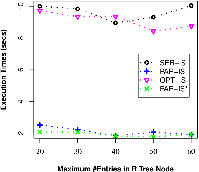 Figure 1
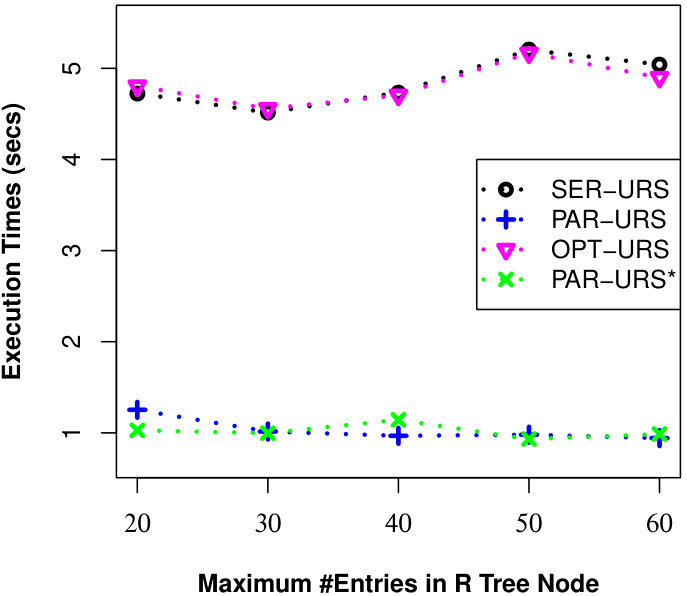 Figure 2
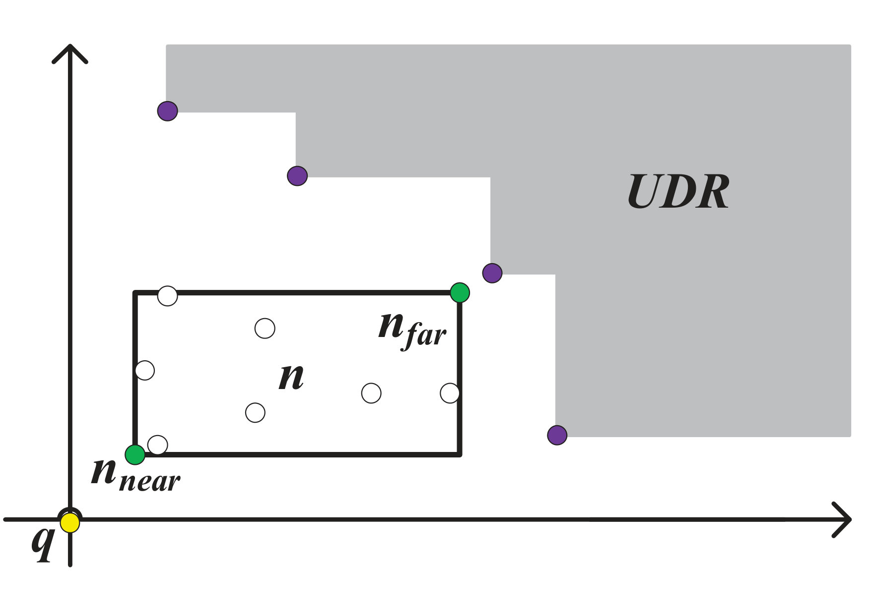 Figure 3
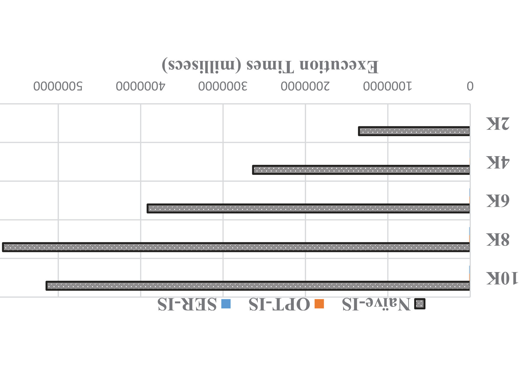 Figure 4
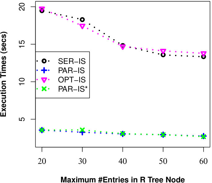 Figure 5
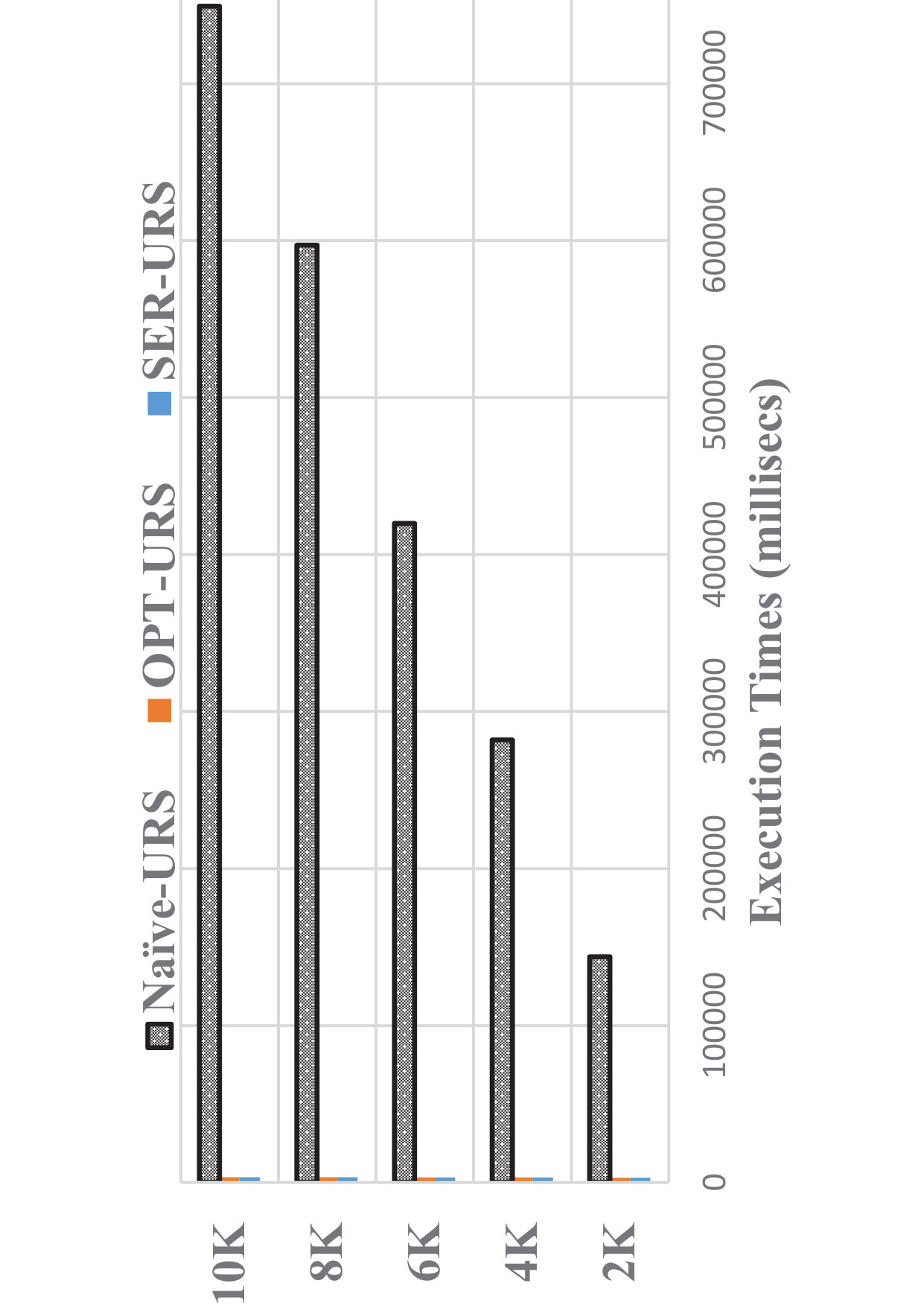 Figure 6
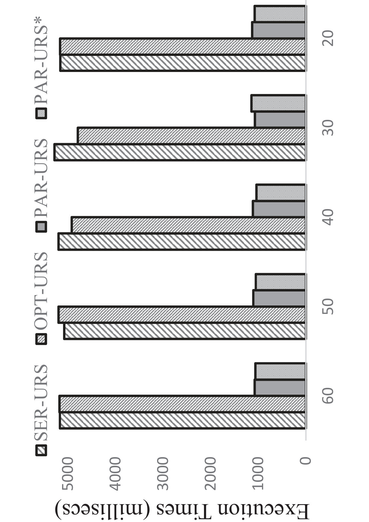 Figure 7
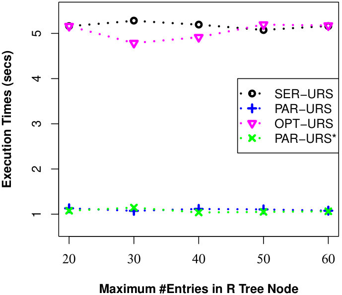 Figure 8
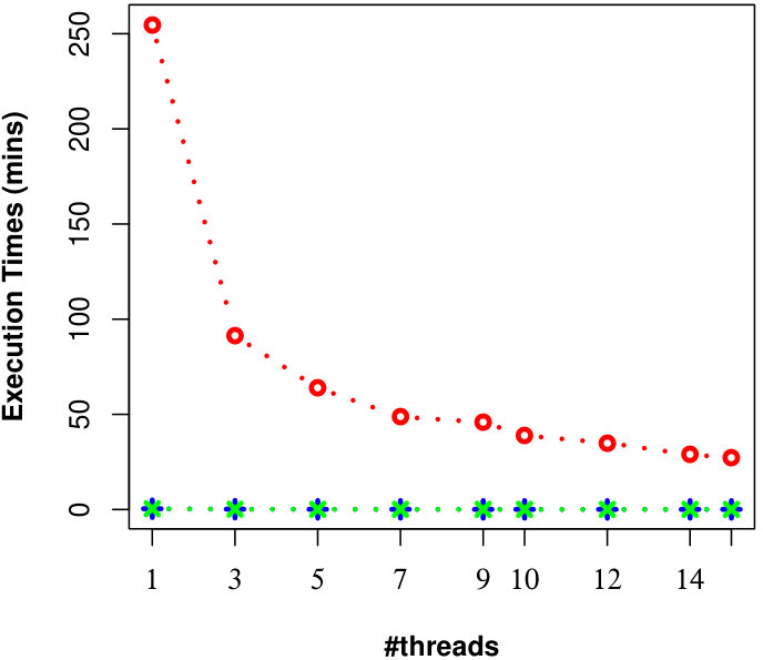 Figure 9
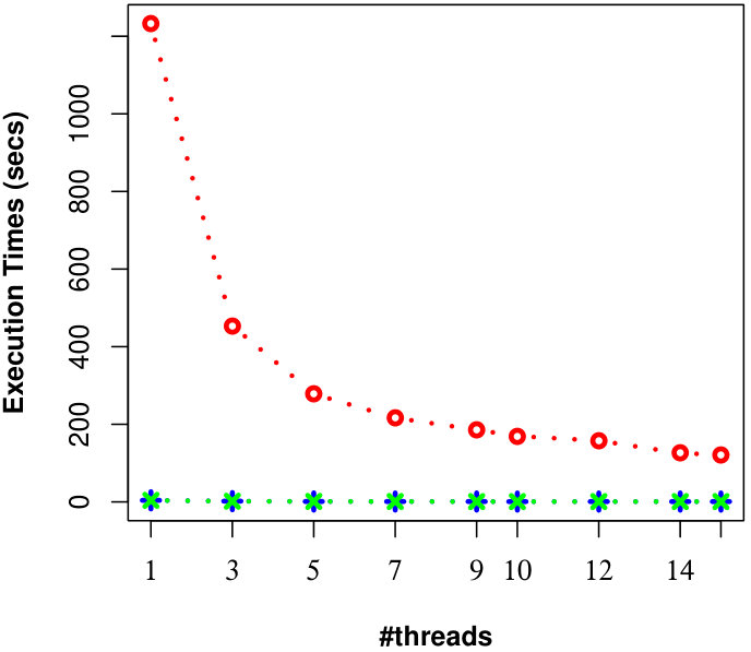 Figure 10
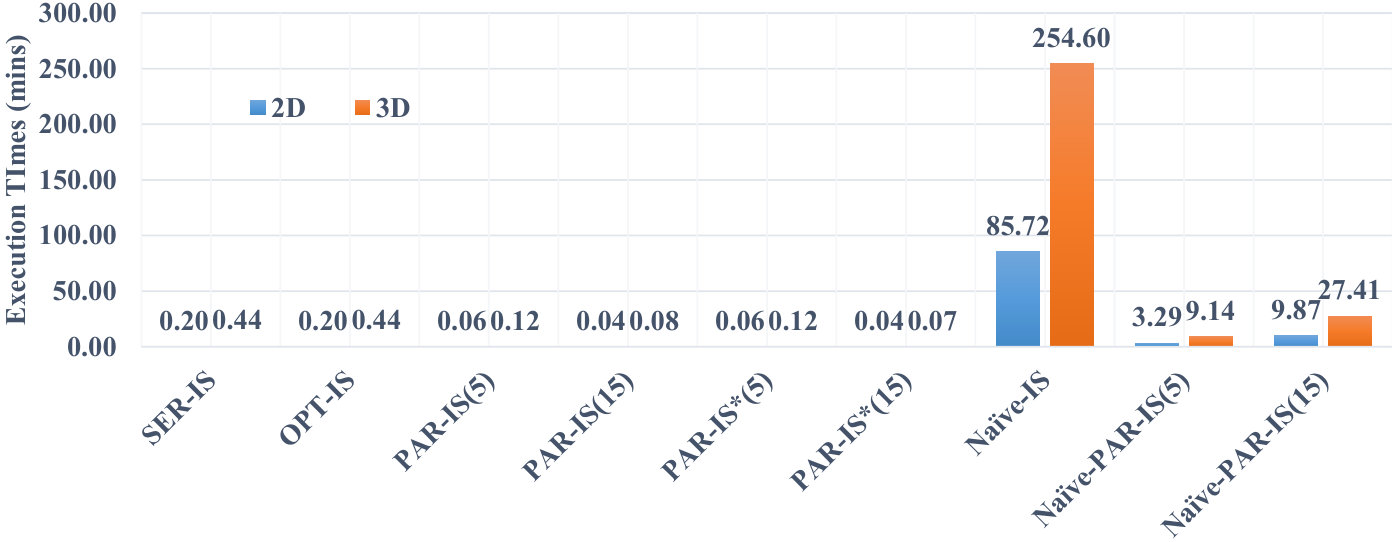 Figure 11
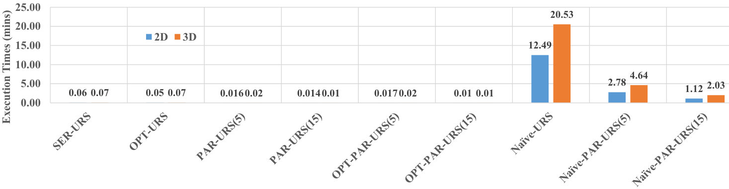 Figure 12
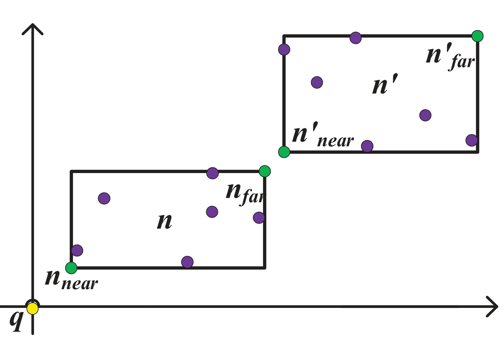 Figure 13
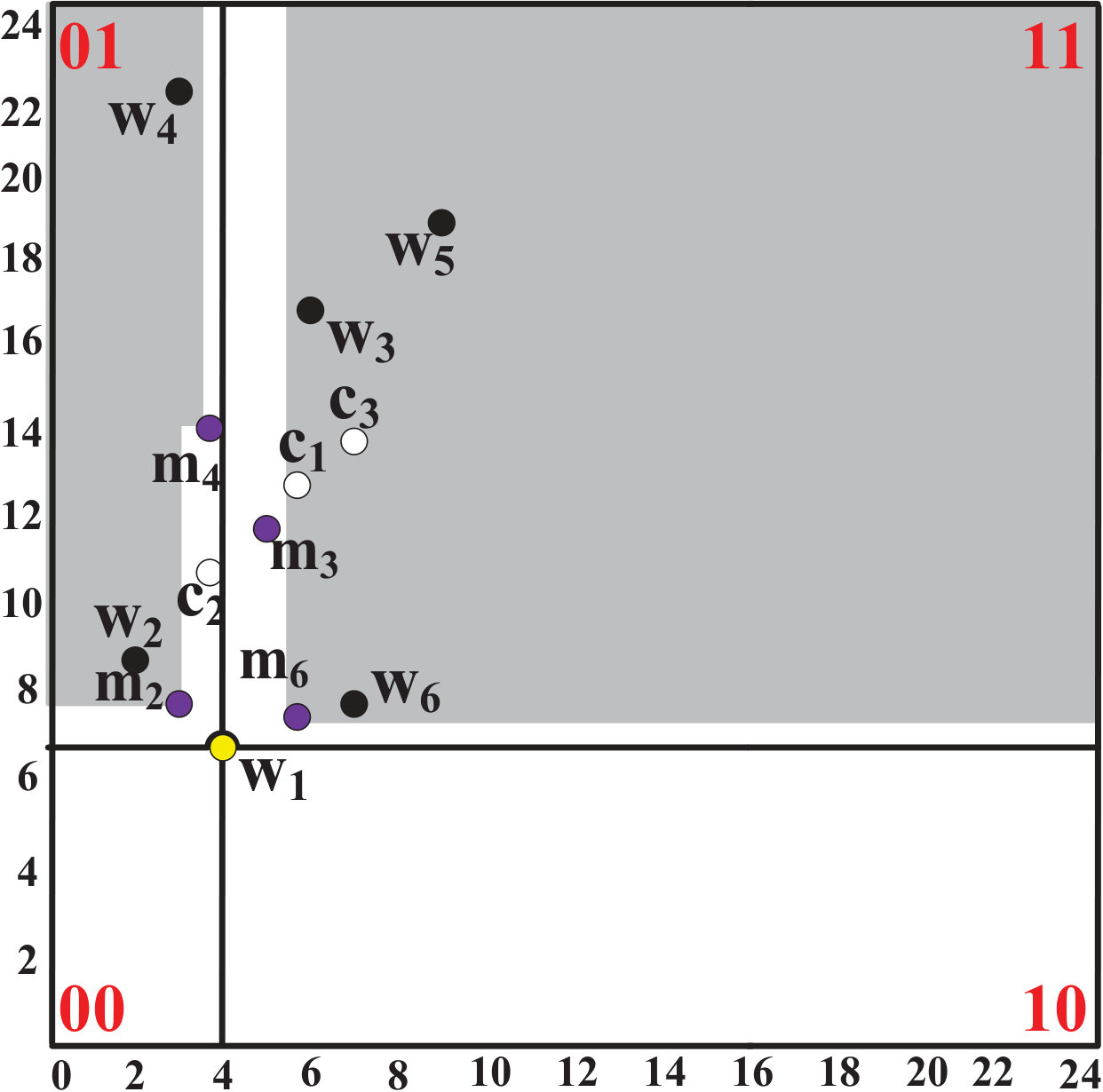 Figure 14
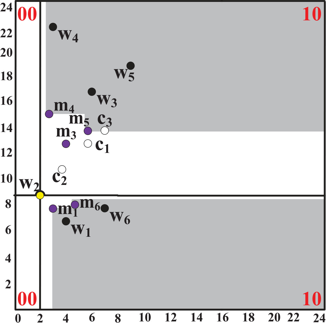 Figure 15
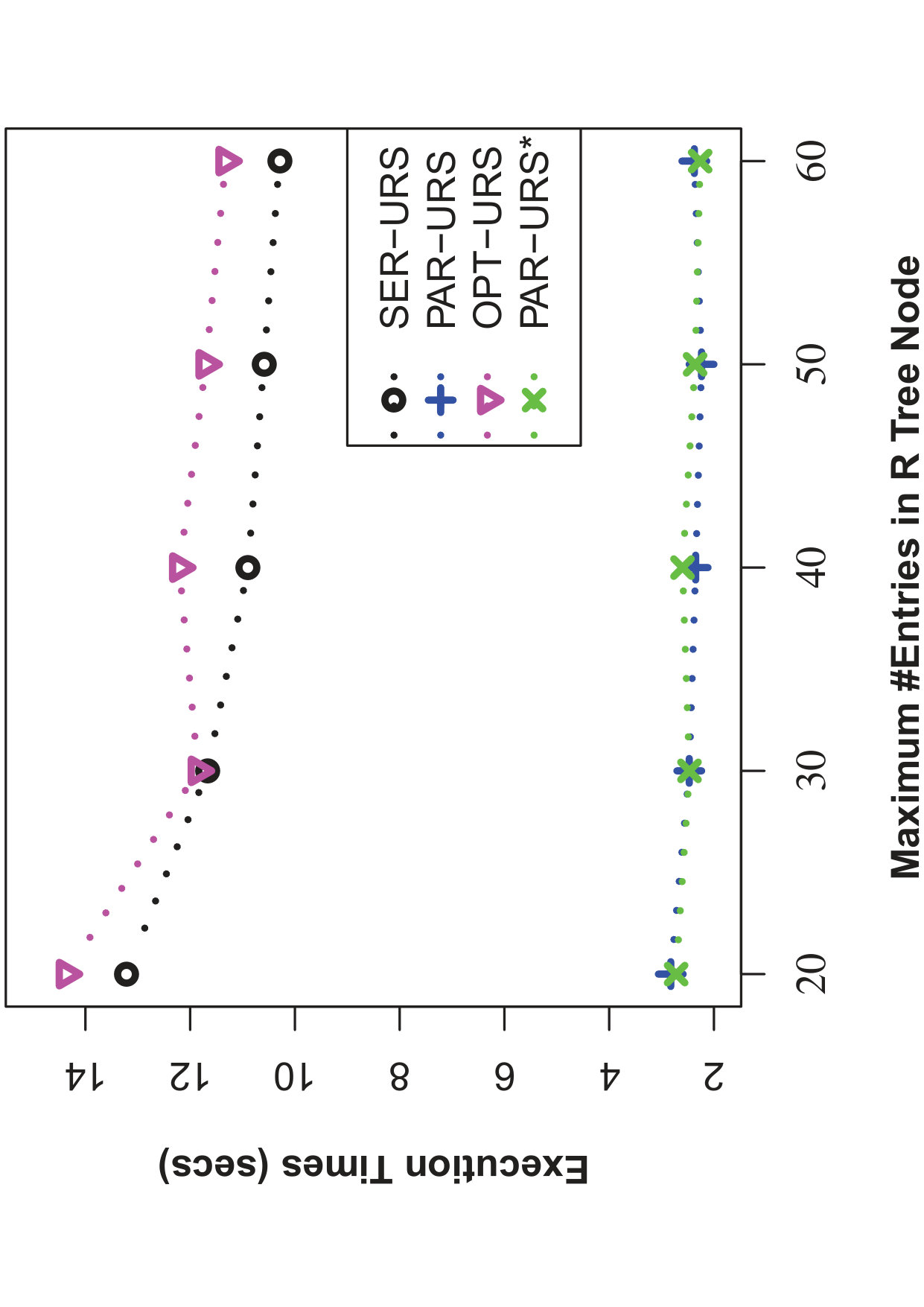 Figure 16
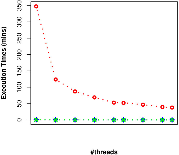 Figure 17
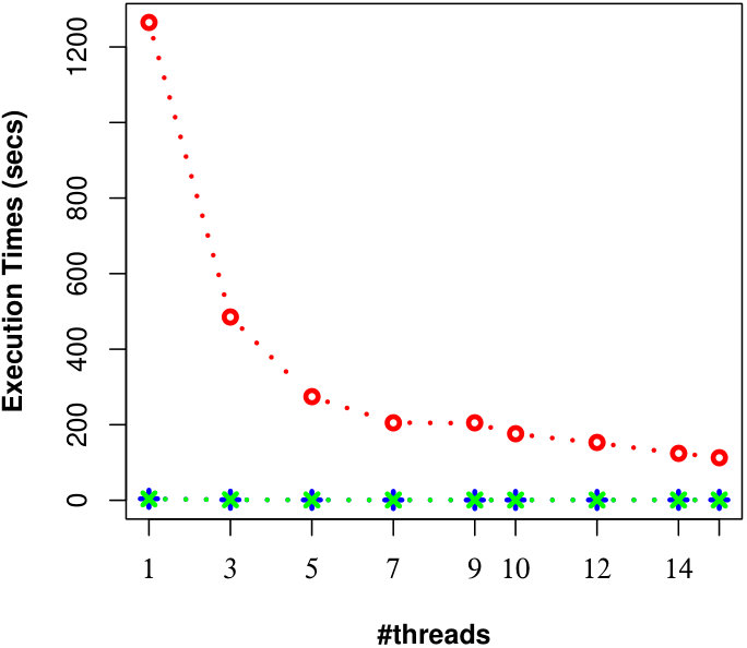 Figure 18
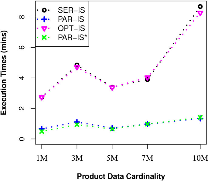 Figure 19
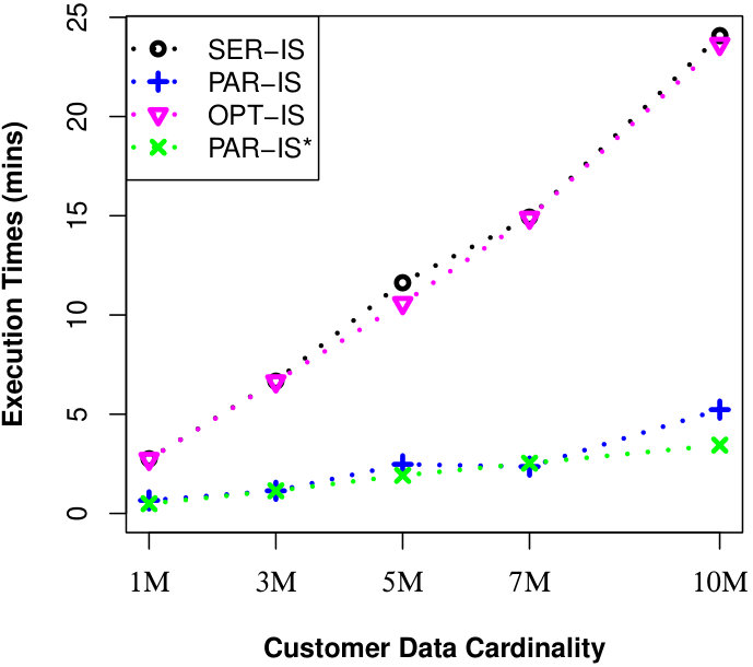 Figure 20
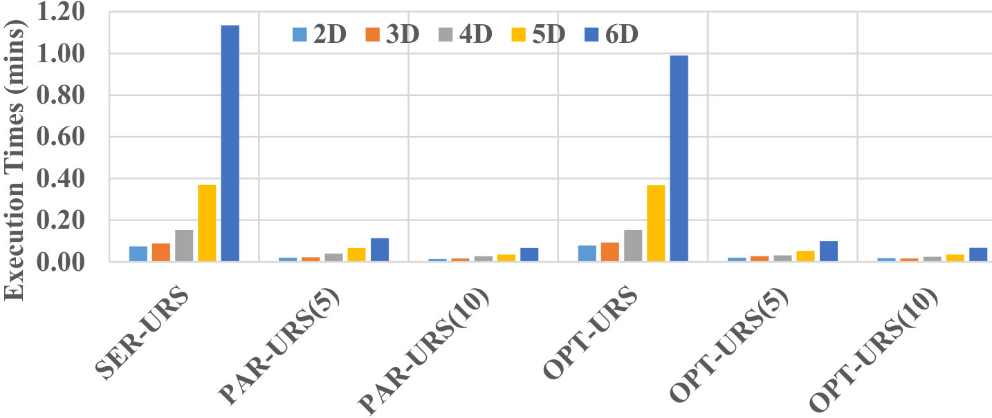 Figure 21
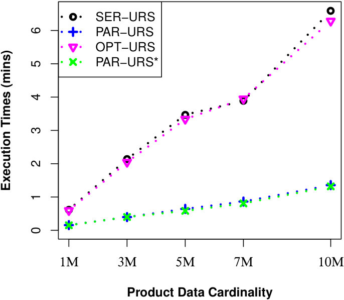 Figure 22
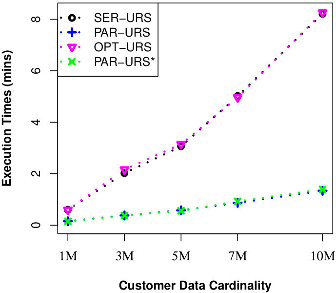 Figure 23
| Parameter | Values |
|---|---|
| Tested Datasets | Real (CarDB), Synthetic (UN, CO, AC) |
| Data Cardinality | 2K, 3K, 4K, 6K, 8K, 10K, 100K, 1M, 3M, 5M, 7M, 10M |
| Dimensionality | D, D, D, D, D |
| No. of Threads | (1 thread per processor) |
| MAX #entries in R-Tree | 20, 30, 40, 50, 60 data objects |
| Cardinality | CarDB (millisecs) | UN (millisecs) | CO (millisecs) | AC (millisecs) | ||||||||
|---|---|---|---|---|---|---|---|---|---|---|---|---|
| SER-URS | OPT-URS | Naïve-URS | SER-URS | OPT-URS | Naïve-URS | SER-URS | OPT-URS | Naïve-URS | SER-URS | OPT-URS | Naïve-URS | |
| Customer(2K) | 3017 | 2990 | 143803 | 2927 | 2991 | 140145 | 3684 | 2940 | 118851 | 3402 | 3246 | 139054 |
| Customer(4K) | 3067 | 3123 | 281937 | 3084 | 3029 | 251026 | 3251 | 3046 | 238909 | 3399 | 3672 | 259967 |
| Customer(6K) | 3162 | 3136 | 419895 | 3233 | 3355 | 380060 | 3166 | 2913 | 337296 | 3402 | 3679 | 356604 |
| Customer(8K) | 3302 | 3288 | 597125 | 3186 | 3278 | 524370 | 3109 | 3106 | 457902 | 3443 | 3696 | 465955 |
| Customer(10K) | 3303 | 3246 | 749371 | 3468 | 3257 | 617057 | 3230 | 3222 | 545728 | 3837 | 4100 | 578158 |
| Customer(100K) | 5077 | 5196 | not executed | 4510 | 4756 | not executed | 4657 | 5134 | not executed | 5201 | 5167 | not executed |
| Cardinality | CarDB (millisecs) | UN (millisecs) | CO (millisecs) | AC (millisecs) | ||||||||
|---|---|---|---|---|---|---|---|---|---|---|---|---|
| SER-IS | OPT-IS | Naïve-IS | SER-IS | OPT-IS | Naïve-IS | SER-IS | OPT-IS | Naïve-IS | SER-IS | OPT-IS | Naïve-IS | |
| Customer(2K) | 5144 | 5149 | 1350344 | 2909 | 2907 | 550090 | 2797 | 2815 | 473691 | 2980 | 2829 | 507864 |
| Customer(4K) | 8438 | 8472 | 2636079 | 3067 | 2962 | 1288985 | 2872 | 2888 | 988031 | 3091 | 2978 | 1005732 |
| Customer(6K) | 11748 | 11516 | 3915923 | 6051 | 6011 | 1609840 | 2958 | 2920 | 1536300 | 3045 | 3015 | 1440399 |
| Customer(8K) | 11953 | 11923 | 5671686 | 6075 | 5998 | 2135613 | 2974 | 2911 | 2109738 | 3111 | 3207 | 1915065 |
| Customer(10K) | 12262 | 12054 | 5143220 | 5969 | 5930 | 3027367 | 2976 | 3116 | 2668434 | 3172 | 3157 | 2273715 |
| Customer(100K) | 13578 | 14116 | not executed | 10595 | 11701 | not executed | 9838 | 10173 | not executed | 9311 | 8430 | not executed |
Peer Reviews
No public reviews on file for this paper yet. If you reviewed it on a platform where reviews are public (OpenReview, ICLR, NeurIPS, ICML), you can paste yours below so the community can read it here.
Videos
No videos yet. Explain this paper in a talk, walkthrough, or lecture? Add one.
Taxonomy
TopicsData Management and Algorithms · Automated Road and Building Extraction · Geographic Information Systems Studies
Computing Influence of a Product through Uncertain Reverse Skyline
Md. Saiful Islam‡1
Wenny Rahayu#2
Chengfei Liu†3
Tarique Anwar†4 and Bela Stantic‡5
‡
†
Griffith University, Gold Coast, Australia
La Trobe University, Melbourne, Australia
Swinburne University of Technology, Melbourne, Australia
{1mdsaiful.islam, 5b.stantic}@griffith.edu.au, [email protected], {3cliu, 4tanwar}@swin.edu.au
Abstract
Understanding the influence of a product is crucially important for making informed business decisions. This paper introduces a new type of skyline queries, called uncertain reverse skyline, for measuring the influence of a probabilistic product in uncertain data settings. More specifically, given a dataset of probabilistic products and a set of customers , an uncertain reverse skyline of a probabilistic product retrieves all customers which include as one of their preferred products. We present efficient pruning ideas and techniques for processing the uncertain reverse skyline query of a probabilistic product using R-Tree data index. We also present an efficient parallel approach to compute the uncertain reverse skyline and influence score of a probabilistic product. Our approach significantly outperforms the baseline approach derived from the existing literature. The efficiency of our approach is demonstrated by conducting extensive experiments with both real and synthetic datasets.
keywords:
UD-Dominance, Uncertain Reverse Skyline, Query Processing Algorithms, Parallel Computing.
1 Introduction
These days we are experiencing voluminous customer preference and the product popularity rating data available from the product related websites, e.g., search queries in CarSales111http://www.carsales.com.au/, YahooAutos222http://autos.yahoo.com/ etc and the product ratings in Amazon333https://www.amazon.com/, eBay444http://www.ebay.com/ etc. The popularity ratings of the products in these sites can be treated as the probabilities by which the products match the customer preferences. Making intelligent use of these customer preference and popularity rating data might help production companies to optimize their (probabilistic) selling strategy or promotion plans and thereafter, increase their revenues [7]. To illustrate the problem settings studied in this paper, consider the datasets of wine products and the customer preferences as given in Fig. 1(b). In general, a product is assumed to be liked by a customer if it closely matches her stated preference. However, the popularity rating of a product may also play an important role in her buying decisions in reality. For example, though matches the preference of the customer better than , still has the chance to attract as its popularity rating is higher than . We argue that both of the above factors need to be modeled in determining the influence of a product and discovering the favorable or popular product set for the manufacturers to sustain in the global market.
The first operator for preference-based data retrieval over certain data is the skyline operator introduced by Börzsönyi et al. [4] to the database research community. Since then, this operator has received lots of attention and is studied extensively in multi-criteria decision making applications ([19], [13], [23], [5], [17], [26], [25] for survey). Given a dataset of products , the standard skyline query returns all products that are not dominated by any other products . A product is considered to dominate another product iff it is as good as in every aspects of , but better than in at least one aspect of . Mathematically, dominates , denoted by , iff: (i) , and (ii) , , assuming that smaller values are preferred in all dimensions, and denote the th dimensional values of and , respectively and is a set of -dimensional data objects. For example, consider the dataset of wine products given in Fig. 1(b)(a), the standard skyline operator [4] on this wine dataset returns as no other wine can dominate these wines in terms of 1- percentage of grape juice content (1-GraCon(%)) and price($).
Though standard skyline queries [4] can trade-off well if there are multiple dimensions of a product and a customer is unable to weight these dimensions, not all customers may prefer to minimize/maximize every dimensional value of a product, rather s/he may like certain range for it, e.g., laptop screen size, GraCon(%) etc. To address this, Papadias et al. [19] propose dynamic skyline query, which retrieves data objects that are not dynamically dominated by another data object w.r.t. a customer preference , where is also a -dimensional data object. Unlike standard skyline queries [4] where the aspects of is directly compared with the corresponding aspects of without considering any customer object, the dynamic skyline query compares the absolute differences of the aspects of and the customer object with the corresponding absolute differences of the aspects of and the customer object in deciding the dominance between and . Mathematically, a data object dynamically dominates another data object w.r.t. a customer object , denoted by , iff: (i) , and (ii) , . For example, consider the dataset of wines given in Fig. 1(b)(a) and the customer preferences in Fig. 1(b)(b), the dynamic skyline query of on the wine dataset returns as no other wines can dominate in view of , i.e., matches the customer preference better than any other wines given in Fig. 1(b)(a).
Both the standard skyline [4] and dynamic skyline [19] queries retrieve data objects from based on the customer’s point of view, not the company’s perspective. Dellis et al. [5] present a new type of skyline queries, called reverse skyline, which retrieves data objects from the company’s point of view. Given a dataset of products , a set of customer preferences and a product query , the reverse skyline query retrieves all customers that include as one of their preferred products. Mathematically, given datasets and and a query , a customer is a reverse skyline of , iff such that (i) , and (ii) , . For example, consider the dataset of wine products given in Fig. 1(b)(a) and the customer preferences in Fig. 1(b)(b), the reverse skyline query of returns as no other wines in Fig. 1(b)(a) can dominate in view of , i.e., is one of the preferred products of the the customer . Like the standard and dynamic skyline queries, reverse skylines are also studied with great importance in the literature, specifically for measuring the influence of a product and evaluating the market research queries ([26], [2], [12], [10] for survey).
Though the above skyline queries are important findings for studying the customer-product relationships over certain data, none of them is applicable over uncertain data. In works [14], [15] Lian et al. present a threshold-based approach for evaluating reverse skyline queries over uncertain data. To find the threshold-based reverse skyline of a probabilistic product , the authors first discover the probable alternative products of a customer , called probabilistic dynamic skyline. The probabilistic dynamic skyline of a customer , denoted by , is computed as follows: , where denotes the dynamic skyline probability of a product w.r.t. and is computed as follows: , denotes the probability of and is a given threshold. Then, the probabilistic reverse skyline of a product , denoted by , consists of all customers that include in its probabilistic dynamic skyline, i.e, . For example, consider the wine products and the customers given in Fig. 1(b). Assume that the popularity ratings in Fig. 1(b)(a) are the probabilities of wines. The probabilistic reverse skyline of retrieves customers and for . Certainly, the study of probabilistic reverse skylines [14], [15] is an advancement for measuring the influence of a product over uncertain data. However, these skylines are not that friendly from usability point of view. (Friendliness) One has to mention the threshold , which is certainly a burden. (Stability) The result set can also vary based on the settings of and therefore, is not stable. (Fairness) Furthermore, it is not favorable towards products with small dynamic skyline probabilities.
Recently, Zhou et al. [28] propose a new skyline query called uncertain dynamic skyline to compute the probable alternative choices for a customer. Unlike probabilistic dynamic skyline [14], [15], the uncertain dynamic skyline [28] is stable and one does not need to provide any threshold value. A product is considered a member of the uncertain dynamic skyline of a customer as long as such that (i) and (ii) . For example, consider the dataset of probabilistic wine products and the customer preferences given in Fig. 1(b), the uncertain dynamic skyline of , denoted by , retrieves and , as no other wines can dynamically dominate them or their dynamic skyline probabilities are greater than these two wines in view of . To compute the influence of a probabilistic product through uncertain dynamic skyline, one has to compute the uncertain dynamic skyline of each customer , i.e., and then, check whether includes . As UDS query is computationally very expensive by itself, computing the influence of a probabilistic product via uncertain dynamic skyline [28] is not efficient.
This paper presents a new skyline query, called uncertain reverse skyline, for measuring the influence of a product in uncertain data settings. We also present efficient pruning ideas and an approach for processing the uncertain reverse skyline query of a probabilistic product. To be specific, our main contributions are as follows:
we introduce a novel skyline query, called uncertain reverse skyline, for measuring the influence of a probabilistic product in uncertain data settings; 2. 2.
we present several pruning ideas and R-Tree data indexing based techniques to compute the uncertain reverse skyline and the influence score of a product in probabilistic databases; 3. 3.
we also present an efficient parallel computing approach for processing the uncertain reverse skyline query of a probabilistic product; and 4. 4.
finally, we demonstrate the efficiency of our approach by conducting extensive experiments with both real and synthetic datasets.
The rest of the paper is organized as follows: Section 2 provides the preliminaries, Section 3 presents the uncertain reverse skyline query and analyses the complexity of computing the influence score of probabilistic product through uncertain reverse skyline, Section 4 describes our approach in detail, Section 5 presents our parallel approach, Section 6 presents the experimental results, Section 7 discusses the related work and finally, Section 8 concludes the paper.
2 Preliminaries
Consider a set of product objects and a set of customer preferences , where a product object and a customer preference are -dimensional points modeled as and , respectively. The denotes the value of the product in the th dimension, whereas the denotes the preferred value of the customer in the th dimension of a product. If the product objects are associated with a probability (e.g., popularity rating), then we call it probabilistic product set. The probability of a product is denoted by . We use product and product object as well as customer and customer preference interchangeably. The query object, denoted by , can represent both a product and a customer.
Definition 1
Dynamic Dominance [19] A product dynamically dominates another product w.r.t. a customer , denoted by , iff the followings hold: (i) and (ii) .
Example 1
Consider the datasets of wine products and the customer . According to the Definition 1, the wine product dominates the wine product w.r.t. the customer , i.e., .
Definition 2
Dynamic Skyline Probability [15, 20]. The dynamic skyline probability of a product w.r.t. a customer , denoted by , is computed as follows:
[TABLE]
Example 2
Consider the probabilistic wine products and customers in Fig. 1(b). As no other objects in dominates w.r.t. , the dynamic skyline probability of w.r.t. is . Since , the dynamic skyline probability of w.r.t. is .
Lemma 1
* iff: (i) and (ii) [28].*
Definition 3
Uncertain Dynamic Dominance (UD-Dominance) [28]. A probabilistic product UD-dominates another probabilistic product w.r.t. a customer , denoted by , iff the followings hold: (i) and (ii) .
Example 3
Consider the probabilistic wine products and customers given in Fig. 1(b). As (see Ex. 1) and also, (see Ex. 2), UD-dominates w.r.t. , i.e., .
Definition 4
Uncertain Dynamic Skyline (UDS) [28]. Given a set of probabilistic products and a customer , the uncertain dynamic skyline of , denoted by , consists of all products such that is not UD-dominated by any other , w.r.t. . Mathematically, .
Example 4
Consider the probabilistic wine products and the customers given in Fig. 1(b). According to Definition 4, the uncertain dynamic skyline of the customer , i.e., , consists of wines and as no other wines in UD-dominates them w.r.t. . Similarly, the and are and , respectively.
Definition 5
Favorite Probability [28]. Given a probabilistic product set , the favorite probability of a product in view of a customer , denoted by , is computed as given as follows:
[TABLE]
The favorability rating of a product w.r.t. a customer set , denoted by , is computed as follows:
[TABLE]
Example 5
Consider the datasets of probabilistic wine products and the customers as given in Fig. 1(b). The favorability rating of w.r.t. the customer set is . Similarly, the favorability rating of w.r.t. is .
3 Uncertain Reverse Skyline
Here, we present a new skyline query, called uncertain reverse skyline query based on UD-Dominance[28].
Definition 6
Uncertain Reverse Skyline (URS). Given a set of probabilistic products , a set of customers and a query product , the uncertain reverse skyline of , denoted by , consists of all customers such that appears in , i.e., . Mathematically, a customer appears in ) iff such that: (a) and (b) .
Example 6
Consider the datasets of probabilistic wines and the customers given in Fig. 1(b). According to Definition 6, the consists of only. The and are and , respectively.
Unlike the probabilistic reverse skyline [15], [16], the uncertain reverse skyline proposed here is user friendly, stable and fair. One does not need to provide the setting of threshold for computing the uncertain reverse skyline and it does not favor the query product over another one unless the query product strictly dominates the other one and the dynamic skyline probability of the query product is better than the other one. The uncertain reverse skyline always returns the same result, i.e., there is no threshold dependency.
Definition 7
Influence. The influence set of a probabilistic product , denoted by , consists of all customers that appear in the uncertain reverse skyline of , i.e, . Given a set of probabilistic products and the customer set , the influence score of a probabilistic product , denoted by , is measured by its favorability rating w.r.t. , i.e., .
Example 7
Consider the datasets of probabilistic wine products and the customers as given in Fig. 1(b). The influence score of wine product is (easy to verify from Ex. 5). Similarly, the influence score of wine product is .
3.1 Complexity Analysis
A naive approach of computing the influence score of a product like the one proposed by Zhou et al. [28] first computes the uncertain dynamic skyline of each customer and then, check whether the includes the product and then computes its influence score by following Eq. 3. However, this approach requires the computation of uncertain dynamic skylines, i.e., . As the UDS query itself is computationally prohibitive, this naïve approach is not efficient enough to compute the influence score of a product , i.e., . The following lemma guides how to efficiently compute through the uncertain reverse skyline of , i.e, .
Lemma 2
.
Proof 3.1**.**
From Definition 7 and Eq. 3, we get:
[TABLE]
Now, we can divide the customers in view of the product into two groups: (a) the customers that appear in the uncertain reverse skyline of , i.e., and (b) the rest, i.e., . Therefore, we can rewrite the above as given as follows:
[TABLE]
According to Definition 6, a product does not appear in the uncertain dynamic skyline of a customer if . Therefore, we get , and the above can be rewritten as given as follows:
[TABLE]
Hence, the lemma, i.e., .
From Lemma 2, we conclude that the efficiency of computing the influence score of a product depends merely on the efficiency of computing its uncertain reverse skyline, i.e., . We present efficient pruning ideas and R-Tree data indexing based techniques for processing the uncertain reverse skyline query of a product in Section 4. As we experience voluminous product and customer data in most data retrieval systems these days, we also present a parallel uncertain reverse skyline query evaluation technique in Section 5, which outperforms its serial counterparts significantly.
4 Our Approach
This section presents our pruning ideas and the detail of uncertain reverse skyline query processing techniques based on probabilistic R-Tree data indexing.
4.1 Pruning Ideas
Definition 4.2**.**
Orthant. Given an object and a query , the orthant of w.r.t. , denoted by , is computed as: iff , otherwise .
A -dimensional query has orthants in total, e.g., the orthants of and are shown as red-colored binary strings in Fig. 2(a) and Fig. 2(b), respectively.
Definition 4.3**.**
Midpoint. The midpoint of a product w.r.t. a query product is computed as given as follows: .
Example 4.4**.**
Consider the datasets of wine products as given in Fig. 1(b)(a). The midpoint of w.r.t. the query product is . Similarly the midpoints of , and w.r.t. are , and , respectively. These midpoints are depicted in Fig. 2(a).
Lemma 4.5**.**
Assume is a midpoint of w.r.t. and the followings hold: (i) ; (ii) ; and (iii) . Then, we get and .
Proof 4.6**.**
As is a midpoint of w.r.t. the product , we get iff [26]. This satisfies the conditions given for Lemma 1, i.e., if conditions (i)-(iii) hold. Now, we get according to Definition 6 as and . Hence, the lemma.
Definition 4.7**.**
UD-Dominance Region (UDR). Given a set of probabilistic products in a -dimensional data space, a region is said to be a UD-dominance region of a product , denoted by , for which , such that the followings hold: (i) , (ii) and (iii) , where is the midpoint of the product w.r.t. .
Example 4.8**.**
Consider the datasets of probabilistic wine products and the customers as given in Fig. 1(b). The UD-dominance regions of and are shown as gray patterned regions in Fig. 2(a) and Fig. 2(b), respectively. Here, the is defined by the midpoints of , and w.r.t. . Similarly, the is defined by the midpoints of , , and w.r.t. .
Lemma 4.9**.**
A customer is not an uncertain reverse skyline of , i.e., if .
Proof 4.10**.**
Assume that . According to the Definition 4.7, such that the midpoint of w.r.t. dominates w.r.t. , i.e., (conditions (i)-(ii)) and also, . Therefore, the does not include according to Definition 4, which implies according to Definition 6.
Definition 4.11**.**
Uncertain Midpoint Skyline. Given a set of probabilistic products , the uncertain midpoint skyline of a probabilistic query product , denoted by , consists of a minimal set of midpoints of the products that defines the UD-dominance region of .
Lemma 4.12**.**
If there are two products and such that the following holds: (i) and (ii) , and , then but , where and are the midpoints of the products and w.r.t. , respectively.
Proof 4.13**.**
Assume that such that and , where is the midpoint of the product , but . This can not happen. Either or such that and , where is the midpoint of a product and . For the former case, the is already correct as will be pruned by from . For the later case, we get as and (transitivity of dominance). Since , can be pruned from by even if . Hence, the lemma.
Example 4.14**.**
The uncertain midpoint skyline of consists of the midpoints of the products , and w.r.t. , i.e., , where , , are the midpoints of , and w.r.t. . Similarly, the consists of the midpoints of the wine products , , and w.r.t. .
4.2 Data Indexing
From Lemma 4.9 and Lemma 4.12, it is obvious that we need to compute the of a probabilistic product to compute its uncertain reverse skyline. Thats is, the midpoints of the probabilistic products that defines the UD-domiance region of the query product . This section presents an efficient approach to approximate the UD-dominance region of a probabilistic product by extending the R-Tree [8] based data indexing for probabilistic product databases, called PR-Tree, which can take advantage of Lemma 4.9 to compute its uncertain reverse skyline. The idea of PR-Tree is to augment each R-Tree node with the maximum and minimum probabilities of its children and store these probabilities in the tree node along with the links to its children. To construct the PR-Tree, we convert each product to its corresponding midpoint and then, insert it in the tree. We also index the customer data by the general R-Tree, which is refereed as CR-Tree in this paper. We use R-Tree to denote either of the trees throughout this paper. In connection with computing the uncertain reverse skyline of a product using R-Tree, we make the following statements.
- •
A midpoint is said to have the same orthant as an R-Tree node , denoted by , if all corners of node have the same orthant w.r.t. as does w.r.t. .
- •
An object dynamically dominates a node w.r.t. a query object , denoted by , if all corners of is dynamically dominated by w.r.t. .
- •
The tree nodes are always accessed in order of their distances to the query product .
4.3 Query Processing
This section describes how to process the uncertain reverse skyline query and the influence (score) of a probabilistic product through its uncertain reverse skyline in detail.
4.3.1 Uncertain Reverse Skyline
While computing the uncertain reverse skyline of a product , we prune a PR-Tree node as per the following lemma.
Lemma 4.15**.**
A PR-Tree node is pruned if such that (i) , (ii) and (iii) , where is the set of midpoints of the products accessed so far in the PR-Tree while computing for and is the midpoint of the product .
Proof 4.16**.**
As all corners of node has the same orthant w.r.t. as does w.r.t. (condition (i)) and any is bounded by the corners of , must have the same orthant w.r.t. as does. Also, as dynamically dominates w.r.t. and is bounded by the corners of , also dynamically dominates w.r.t. , i.e., . Therefore, , if and , we also get and (condition (iii)), which implies can be pruned. Hence, the lemma.
While computing the uncertain reverse skyline of a product , we prune a CR-Tree node as per the following lemma.
Lemma 4.17**.**
A CR-Tree node is pruned if such that (i) and (ii) .
Proof 4.18**.**
As all corners of node has the same orthant w.r.t. as does w.r.t. (condition (i)) and any is bounded by the corners of , must have the same orthant w.r.t. as does. Also, as dynamically dominates w.r.t. (condition (ii)) and is bounded by the corners of , dynamically dominates w.r.t. , i.e., . Therefore, such that , where is the corresponding product of the midpoint and as , which implies can be pruned. Hence, the lemma.
The steps of computing the uncertain reverse skyline of a product , i.e., , with R-Trees are listed as follows:
Firstly, we convert the products into their midpoints w.r.t. and index them into a PR-Tree. 2. 2.
We initialize to an empty set. Then, we retrieve the children of the root node of the PR-Tree and insert them into a mean-heap . We repeatedly retrieve the front entry from until becomes empty and do the following: ignore iff such that (i) and (ii) (Lemma 4.15), otherwise, insert its children into if is a non-leaf node, else add the midpoint contained in into iff , where is the corresponding product of the midpoint in . 3. 3.
We index the customer data into a CR-Tree and initialize to an empty set. Then, we retrieve the children of the root node of the CR-Tree and insert them into a mean-heap . We repeatedly retrieve the front entry from until becomes empty and do the following: ignore iff such that (i) and (Lemma 4.17), otherwise, insert its children into if is a non-leaf node, else add the contained in into .
The above steps are pseudocoded in Algorithm 1.
Lemma 4.19**.**
Algorithm 1 computes accurately the uncertain reverse skyline of an arbitrary probabilistic product .
Proof 4.20**.**
The computation of the uncertain reverse skyline of , i.e., , starts scanning the products , then converting them into their corresponding midpoints w.r.t. and thereafter, inserting them into the PR-Tree as given in lines 2-3. Then, we initialize to and insert the children of PR-Tree root into the min-heap in lines 4-5. The lines 6-13 repeatedly retrieve the front entry of until is empty and prune (PR-Tree node) as per Lemma 4.15, otherwise, insert the children of into if is an internal node, else add the midpoint contained in (leaf node) into the only if to make sure that if such that and hold, can be pruned by as per Lemma 4.9, where is the corresponding product of in . As the entries (PR-Tree nodes) in are accessed in order of their distances to , the computed in lines 6-13 is minimal and correct. Now, we initialize to , constrcut CR-Tree of the customers and insert the children of the CR-Tree root into the min-heap in lines 14-16. The lines 17-24 repeatedly retrieve the front entry of until is empty and prune (CR-Tree node) as per Lemma 4.17, otherwise, insert the children of into if is an internal node, else add the customer contained in (leaf node) into the as per the Definition 6. Hence, the lemma.
4.3.2 Influence Score
As per Eq. 4, we need to compute the dynamic skyline probability of each product for each to compute the influence score of the query product . To achieve this, we first compute the uncertain reverse skyline of , i.e., by Algorithm 1. Then, we compute the dynamic skyline probability of each product for each as per the approach proposed in [28]. This idea is pseudocoded in Algorithm 2. Though, we adopt the approach proposed in [28] for computing the dynamic skyline probability in Algorithm 2, there is a significant difference between our approach and the approach proposed in [28] for computing . The approach proposed in [28] computes the of each customer irrespective of whether is in or not to compute , which we don’t do in our approach. Therefore, our approach is more efficient than the naïve approach proposed in [28] for computing the influence score of an arbitrary query product .
4.3.3 Optimization
Assume that is the farthest and is the nearest corner of a R-Tree node w.r.t. as shown by the green-colored bulleted objects in Fig. 3. If is a PR-Tree node, also assume that and , where is the corresponding product in of the midpoint .
The following lemma guides how to prune a PR-Tree node by comparing it with another PR-Tree node while computing the uncertain midpoint skyline of an arbitrary query product , i.e., .
Lemma 4.21**.**
A PR-Tree node can be pruned if such that (i) , (ii) and (iii) .
Proof 4.22**.**
Assume that and such that and , where is the corresponding product in of the midpoint , i.e., . Now, there must exist a midpoint such that because of conditions (i) and (ii) as follows: (transitivity of dominance). Now, because of condition (iii), where is the corresponding product in of the midpoint , which implies . Therefore, we can still prune by even if we prune . Hence, the lemma.
Lemma 4.23**.**
The customers in a CR-Tree node can be safely added to if such that the followings hold: (i) and (ii) .
Proof 4.24**.**
Assume that and the conditions (i)-(ii) are true, but . We prove that is incorrect. As such that and is bounded within the region of node , we get . Therefore, must be in . Hence, the lemma.
The above optimization heuristics, i.e., Lemma 4.21 and Lemma 4.23 are pseudocoded in Algorithm 3. The difference between Algorithm 1 and Algorithm 3 is that Algorithm 3 applies PR-Tree node to node pruning on after inserting the children of an entry into while computing (lines 10-12) and adds the customers of a CR-Tree non-leaf node into if the conditions in Lemma 4.23 are satisfied without inserting the children into (lines 22-23). The optimization of influence score computation in Algorithm 2 is done by replacing Algorithm 1 with Algorithm 3 in line 2 for computing the uncertain reverse skyline of .
5 Parallel Approach
This section presents an efficient approach of computing the uncertain reverse skyline and the influence score of a product by parallelizing their evaluations for today’s data intensive systems involving millions of customer objects.
5.1 Computing Environment
We assume a simplified computing environment for evaluating uncertain reverse skyline queries in parallel in which a master processor, denoted by , is responsible for coordinating and managing the independent tasks carried out by the worker processors, denoted by . A worker processor receives input data from the master and the task type, finishes the task accordingly and sends the processed result back to the master processor. The master processor may pre-process the input data before sending them to the workers. The master processor finalizes the result in one or more rounds. We also assume that the communications and synchronizations between the master processor and the worker processors are integral part of this environment, and the computing powers of all worker processors are the same.
5.2 Parallel Uncertain Reverse Skyline
The parallel steps of computing the uncertain reverse skyline of a probabilistic product , i.e., , in two rounds are listed as follows:
In the first round, the master divides into chunks (such that ) and sends these chunks and the query product to its workers. 2. 2.
A worker processor converts the products into their midpoints w.r.t. and index them into its local PR-Tree. Then, the worker computes the local uncertain midpoint skyline by following the same technique as given in Step 2 in Section 4.3.1. 3. 3.
Then, the master does the followings: (i) collects all local s from its workers and insert them into a min heap ; (ii) initializes to and (iii) repeatedly retrieves the front entry from until it becomes empty and does the following: adds to if such that: and , otherwise ignore . 4. 4.
In the second round, the master divides into chunks (such that ) and sends these chunks and the global to its workers. 5. 5.
A worker processor index into its local CR-Tree. Then, the worker computes the local uncertain reverse skyline by following the same technique as given in Step 3 in Section 4.3.1 6. 6.
Finally, the master collect all local s from its workers into the global .
The above steps are pseudocoded in Algorithm 4 as explained below. The master processor partitions the product data equally for the workers in line 2. The master processor then sends the query product and the partitioned data to the corresponding worker processor in lines 4-5. In lines 6-8, the worker processor converts into the corresponding midpoints , constructs the local PR-Tree and computes the local uncertain midpoint skyline by calling localMidpointSkyline(, ) method which implements Step 2. Once computed, sends the local to the master in line 8. The master computes the global uncertain midpoint skyline by calling globalMidpointSkyline(, ) method which implements Step 3) in line 9. The master processor now partitions the customer data equally for the workers in line 10 and then, sends the global and to the corresponding worker in lines 12-13. The worker processor constructs the local CR-Tree and computes the local by calling method localURS(, , ) which implements step 5 in lines 14-15. Finally, the local are accumulated by the master into the global uncertain reverse skyline in line 16 of Algorithm 4.
Lemma 5.25**.**
The Algorithm 4 accurately computes the uncertain reverse skyline of an arbitrary query product .
Proof 5.26**.**
Firstly, we prove that the global uncertain midpoint skyline, i.e., computed by Algorithm 4 is correct. The local midpoint skyline of is correct for the partition as we prove for in Algorithm 1. Now, Algorithm 4 computes the global by accumulating the local s into the mean heap and thereafter, accessing the midpoints in in order of their distances to . A midpoint is added to the global iff it’s filtering capability cannot be achieved by another midpoint already existing in . Therefore, the global can filter the customers that would be filtered by local s, i.e., the global is correct and minimal. Finally, the worker processor computes the local for the customer set based on the global as we compute for in Algorithm 1. As the selection of customers in the uncertain reverse skyline set of are mutually independent, the global accumulated in the master is correct. Hence, the lemma.
5.3 Parallel Influence Score
This section presents an approach for computing the influence score of an arbitrary query product in parallel. More specifically, we parallelize the computation of the dynamic skyline probabilities of each product for each . Our approach is significantly different from the approach proposed in [28]. The approach in [28] computes the favorite probability by executing the uncertain dynamic skyline query of each in different processing nodes without partitioning . In our approach, we partition not only , but also , and execute the uncertain dynamic skyline query only for , not for each as suggested in Lemma 2. Our approach is described below.
Firstly, we compute the uncertain reverse skyline of , i.e., by calling Algorithm 4. Then, each worker constructs the PR-Tree on without converting it to midpoints. Then, we compute two sets of products and for each customer on each partition locally by following the same technique described in [28]. Once the local and product sets are calculated, we accumulate them into the sets and in the master. We move a product from to iff such that and . We also update by ignoring all iff such that and .
Once the and product sets are computed for each , we update the dynamic skyline probabilities of the 555The dynamic skyline probability of a is i.e., , as such that . product set in parallel. To achieve this, firstly we compute the dominating points for each on each partition by running window/range query for it locally. Once done for each partition, we update the dynamic skyline probabilities of the products by their dominating products and compute the favorite probability of each in the master. Once the favorite probabilities are computed, the influence score of the query product is computed by following Eq. 4. The above parallel steps are pseudocoded in Algorithm 5.
Lemma 5.27**.**
Algorithm 5 accurately computes the influence score of an arbitrary query product in parallel.
Proof 5.28**.**
Here, we prove that we accurately compute UDS and UDSScan product sets for each customer in Algorithm 5. The local and product sets are computed by following the same the technique as described in [28]. Once these sets are computed locally, we accumulated them in the master for further refinement. The refinement ensures that set includes only non-dominating products for a customer . Similarly, the set includes only products that are not UD-dominated by any other products. Finally, the algorithm computes the dominating products for each product w.r.t. by executing range query on each partition w.r.t. and . The discovery of these dominating products in each partition are independent from one partition to another. Therefore, the final UDS and UDSScan (along with the dominating products of each ) product sets are accurate. Hence, the lemma.
5.4 Optimization
An optimized version of Algorithm 4 can be achieved by applying Lemma 4.21 and Lemma 4.23 while computing the local and of , respectively, as we apply these lemmas in Algorithm 3. An optimized version of Algorithm 5 can also be achieved by executing optimized version of Algorithm 4 while computing the of in line 2.
6 Experiments
This section compares the efficiencies of different approaches for evaluating the uncertain reverse skyline queries and computing the influence score of a product in probabilistic databases.
6.1 Datasets, Queries and Environment
Datasets: We evaluate the efficiency of our pruning ideas and techniques for processing the uncertain reverse skyline queries using real CarDB666https://autos.yahoo.com/ data which consists of car objects. The CarDB is a six-dimensional dataset with attributes: make, model, year, price, mileage and location. We consider only the three numerical attributes year, price and mileage in our experiments after normalizing them into the range . We randomly select half of the car objects as products and the rest as the customer preferences. We also assign random probabilities to the car objects. The synthetic data experiments include data: uniform (UN), correlated (CO) and anti-correlated (AC), consisting of varying number of products, customers and dimensions. The cardinalities of the synthetic datasets range from K to M. The dimensionality () of the datasets varies from 2 to 6.
Test Queries: The test queries are generated (synthetic) and selected (CarDB) randomly by following the distribution of the respective datasets. Again, the query products are assigned with random probabilities.
Computing Environment: We develop our algorithms in Java and execute them in Swinburne HPC system 777http://www.astronomy.swin.edu.au/supercomputing/ with 115 processors and maximum 60GB main memory, where the parallel computing environment (master-worker) is simulated with Java multi-threading and LOCK-based synchronization. The above parameters are summarized in Table 1.
6.2 Tested Algorithms
To compare the efficiency of evaluating uncertain reverse skyline queries, we tested the following algorithms: Serial URS (SER-URS) - Algorithm 1, Optimized URS (OPT-URS) - Algorithm 3, Parallel URS (PAR-URS) - Algorithm 4 and Optimized Parallel URS (PAR-URS∗) - Optimized Algorithm 4. The naïve algorithm proposed in [28] and its parallel version are called Naïve-URS and Naïve-PAR-URS, respectively. To improve the performance of Naïve-URS and Naïve-PAR-URS, we do not update the dynamic skyline probabilities of the products that appear in the UDSScan set of each customer as we do not need to know the dynamic skyline probabilities of these products for the inclusion of the customer in , we only need to know whether appears in the UDS or UDSScan sets of .
To compare the efficiency of computing the influence score of a probabilistic product, we tested the efficiencies of the following algorithms: Serial Influence Score (SER-IS) - Algorithm 2, Optimized Influence Score (OPT-IS) - Optimized Algorithm 2, Parallel Influence Score (PAR-IS) - Algorithm 5 and Optimized Parallel Influence Score (PAR-IS∗) - Optimized Algorithm 5. The naïve algorithm [28] and its parallel version are called Naïve-IS and Naïve-PAR-IS, respectively.
6.3 Efficiency Study
This section studies the efficiency of our proposed algorithms by comparing the execution times with the naïve approach proposed in [28] from the following perspectives.
6.3.1 Effect of data cardinalities
Here, we examine the effect of data cardinality (#customers) on the efficiency of processing uncertain reverse skyline queries and computing influence score of a probabilistic product by different approaches on the tested datasets. We set = 100K, = 2 and vary from 2K to 100K. We also set MAX #entries in a R-Tree node to 50. We run a number of queries and the results of evaluating a uncertain reverse skyline query and computing the influence score of a probabilistic product on average are shown in Table 2 and Table 3, respectively. It is evident that the naïve approach [28] is not scalable, whereas our approaches are scalable and can finish their executions within seconds even for 100K customers (naïve approach [28] is not executed as it takes hours to finish). We see that the speed-ups achieved by our approach over the naïve approach [28] are hugely significant.
To justify the scalability of our approaches for millions of data objects, we perform another two experiments in UN dataset. For the first experiment, we set M and vary from M to M. For the second experiment, we set M and vary from M to M. For both experiments, we also set = 2 and MAX #entries in a R-Tree node to 50. Finally, we run a number of queries and the results of evaluating a uncertain reverse skyline query and computing the influence score of a probabilistic product on average are shown in Fig. 4 and Fig. 5, respectively. We observe that our approaches can finish their executions within few minutes for millions of data objects.
6.3.2 Effect of data dimensions
Here, we examine the effect of data dimensionality on the efficiency of processing uncertain reverse skyline queries and computing the influence scores of probabilistic products by different approaches on CarDB two-dimensional (2D) and three-dimensional (3D) datasets. We set = 100K, =10K, #threads to 5 and 15 for PAR-URS, PAR-URS*, Naïve-PAR-URS, PAR-IS, PAR-IS* and Naïve-PAR-IS, and the MAX #entries in a R-Tree node to 50. We run a number of queries and the results of processing uncertain reverse skyline of a query and computing the influence score of a probabilistic product on average are shown in Fig. 6 and Fig. 7, respectively. We observe that the naïve approach[28] takes minutes to finish its execution in 3D data even with 15 threads (processors). The execution times get more worse for increased customer cardinality and dimensionality. On the other hand, all of our proposed approaches scale very well and finish their executions within seconds. We also perform another experiment in higher dimensions for UN dataset with varying from 2 to 6 for testing the efficiency of evaluating the uncertain reverse skyline of a query. For this experiment, we set and to K, and the MAX #entries in a R-Tree node to 50. The results are shown in Fig. 8. We observe that all of our approaches can finish their executions within 2 minutes. Therefore, we claim that our approaches are scalable even in higher dimensions.
6.3.3 Effect of threads
Here, we examine the effect of #threads on the efficiency of processing uncertain reverse skyline queries and computing the influence scores of probabilistic products in parallel by different approaches on CarDB and UN datasets. We set = 100K, =10K, = 3, MAX #entries in a R-Tree node to 50 and vary #threads from 1 to 15. We run a number of queries and the results of evaluating an uncertain reverse skyline query and computing the influence score of a probabilistic product on average for different #threads are shown in Fig. 9 and Fig. 10, respectively. It is evident that the naïve approach[28] is not scalable even if we increase the #threads, whereas our approaches are scalable and can finish their executions within seconds with less #threads.
6.3.4 Effect of R-Tree parameters
Here, we examine the effect of R-Tree parameters (MAX #entries in a R-Tree node) on the efficiency of processing uncertain reverse skyline queries and computing the influence scores of probabilistic products by different approaches on CarDB and AC datasets. Here, we set = 100K, =100K, #threads to 10 for PAR-URS and PAR-URS*, = 2 and vary MAX #entries in a R-Tree node from 20 to 60. We run a number of queries and the results of evaluating an uncertain reverse skyline query and computing the influence score of a probabilistic product on average are shown in Fig. 11 and Fig. 12, respectively. We observe that efficiency improves in general in SER-URS and OPT-URS with the increased MAX #entries in a R-Tree node. However, we observe an exception in their parallel evaluations. We also observe that the efficiencies of different approaches improve if we increase the MAX #entries in a R-Tree node in general except for SER-IS in AC dataset. We believe that the efficiency depends on many factors including data distribution in different threads (processors) and #threads, not only on the MAX #entries in a R-Tree node.
6.4 Summary
We experimentally demonstrate (prove theoretically in Section 3.1) that the naïve approach proposed in [28] is not scalable for computing the influence score of a probabilistic product. The computation of the influence score of a probabilistic product through uncertain reverse skyline in uncertain data is scalable for millions of customer and product data objects, and can finish executions within few minutes.
7 Related Work
Reverse Skyline Queries and Related Studies. Dellis et al. [5] are the first to present reverse skyline query to the database community. Later, Wu et al. [26] propose an efficient approach for computing the influence of a product through its reverse skyline, where the influence set consists of the member of the reverse skyline query results. Then, [6] propose an approach for evaluating reverse skyline queries with non-metric similarity measures. Wang et al. [24] propose an energy efficient approach for evaluating reverse skyline queries over wireless sensor networks. Arvanitis et al. [2] extends this idea for computing the -most attractive candidates (-MAC) from a given set of products that maximizes the size of their joint influence set (score). Islam et al. [12] propose an approach to answer how to turn up a given customer into the reverse skyline query result of an arbitrary query product. Recently, Islam et al. [10] present an approach for computing the -most promising products (-MPP), which assigns equal probabilities to the products appearing in the dynamic skyline of a customer and selects a subset of given products to maximize their joint probabilistic influence score. All of the above works are in certain data settings. Lian et al. [14], [16] extends the idea of reverse skyline query in uncertain data settings. However, the probabilistic reverse skylines proposed in [14], [16] lack friendliness, stability and fairness as per [28]. Zhou et al. [28] propose uncertain dynamic skyline and an approach to compute top- favorite probabilistic products through uncertain dynamic skyline. However, the approach proposed in [28] is not efficient as discussed in Section 3.1. This paper presents uncertain reverse skyline query to efficiently evaluate the influence of an arbitrary probabilistic product in uncertain data settings. Unlike [14], [16], the uncertain reverse skyline proposed here is user friendly, stable and fair.
Parallelizing Reverse Skyline Queries. Though there exist many works on parallelizing the standard skyline queries ([9], [18], [1], [22], [3], [27] for survey), there are only few works devoted to parallelizing the reverse skyline queries. Park et al. [21] propose an approach for parallelizing both dynamic and reverse skyline queries in MapReduce by inventing a novel quad-tree based data indexing. Later, the authors extend their quad-tree based data indexing in [20] for evaluating probabilistic dynamic and reverse skylines. Recently, Islam et al. [11] propose an advancement of the quad-tree based data indexing proposed in [21] for evaluating the dynamic skyline, monochromatic and bichromatic reverse skylines in parallel. Here, we propose an efficient approach for parallelizing the computation of uncertain reverse skyline query result and the influence score of an arbitrary probabilistic product using R-Tree. Our approach for computing the influence score of a probabilistic product is significantly different from the one proposed in [28]. Here, we only compute the dynamic skyline probabilities of the products that appear in the uncertain dynamic skyline of the customers existing in the uncertain reverse skyline of the query product, not for all customers in the dataset.
8 Conclusion
This paper presents a novel skyline query, called uncertain reverse skyline, for measuring the influence of an arbitrary probabilistic product in uncertain data settings. We propose efficient pruning ideas and techniques for processing the uncertain reverse skyline and the influence score of a query product in probabilistic databases using R-Tree. We also present a parallel approach for evaluating the uncertain reverse skyline query and the influence score of a probabilistic product, which outperforms its serial counterpart. We conduct experiments with both real and synthetic datasets and compare our results with the existing baseline approach to demonstrate the efficiency of our approach.
9 Acknowledgment
The research of C. Liu and T. Anwar is supported by the ARC discovery projects DP160102412 and DP170104747.
The reference list from the paper itself. Each links out to its DOI / PubMed record.
- 1[1] F. N. Afrati, P. Koutris, D. Suciu, and J. D. Ullman. Parallel skyline queries. Theory Comput. Syst. , 57(4):1008–1037, 2015.
- 2[2] A. Arvanitis, A. Deligiannakis, and Y. Vassiliou. Efficient influence-based processing of market research queries. In CIKM , pages 1193–1202, 2012.
- 3[3] K. S. Bøgh, S. Chester, and I. Assent. Work-efficient parallel skyline computation for the GPU. PVLDB , 8(9):962–973, 2015.
- 4[4] S. Börzsönyi, D. Kossmann, and K. Stocker. The skyline operator. In ICDE , pages 421–430, 2001.
- 5[5] E. Dellis and B. Seeger. Efficient computation of reverse skyline queries. In VLDB , pages 291–302, 2007.
- 6[6] P. M. Deshpande and D. Padmanabhan. Efficient reverse skyline retrieval with arbitrary non-metric similarity measures. In EDBT , pages 319–330, 2011.
- 7[7] S. Fay and J. Xie. Probabilistic goods: A creative way of selling products and services. Marketing Science , 27(4):674–690, 2008.
- 8[8] A. Guttman. R-trees: A dynamic index structure for spatial searching. In SIGMOD , pages 47–57, 1984.