Parallel Optimization of Polynomials for Large-scale Problems in Stability and Control
Reza Kamyar

TL;DR
This paper develops parallel algorithms for large-scale polynomial optimization problems in control theory, enabling stability analysis of high-dimensional systems using supercomputers to handle complex SDPs efficiently.
Contribution
It introduces parallel algorithms for solving large SDPs in stability analysis, leveraging problem structure and supercomputing resources for scalability.
Findings
Efficiently analyzes systems with 100+ dimensions
Parallel algorithms utilize hundreds to thousands of processors
Demonstrates scalability on supercomputers
Abstract
In this thesis, we focus on some of the NP-hard problems in control theory. Thanks to the converse Lyapunov theory, these problems can often be modeled as optimization over polynomials. To avoid the problem of intractability, we establish a trade off between accuracy and complexity. We develop a sequence of tractable optimization problems - in the form of LPs and SDPs - whose solutions converge to the exact solution of the NP-hard problem. However, the computational and memory complexity of these LPs and SDPs grow exponentially with the progress of the sequence - meaning that improving the accuracy of the solutions requires solving SDPs with tens of thousands of decision variables and constraints. Setting up and solving such problems is a significant challenge. The existing optimization algorithms and software are only designed to use desktop computers or small cluster computers -…
Click any figure to enlarge with its caption.
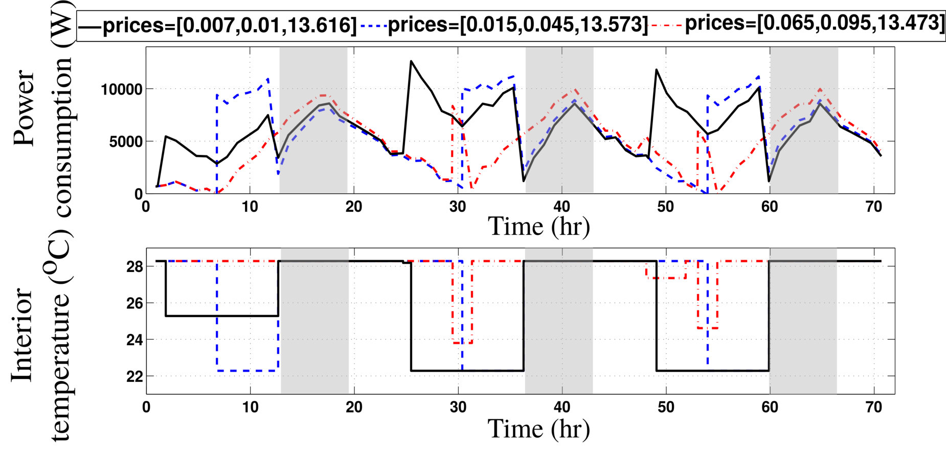 Figure 1
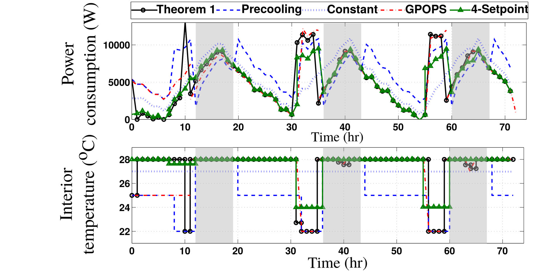 Figure 2
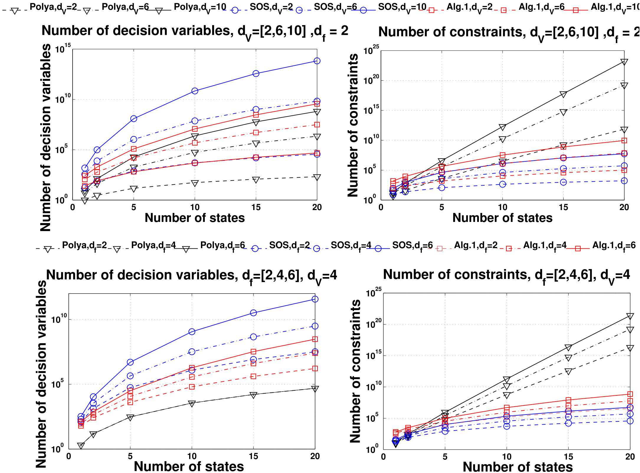 Figure 3
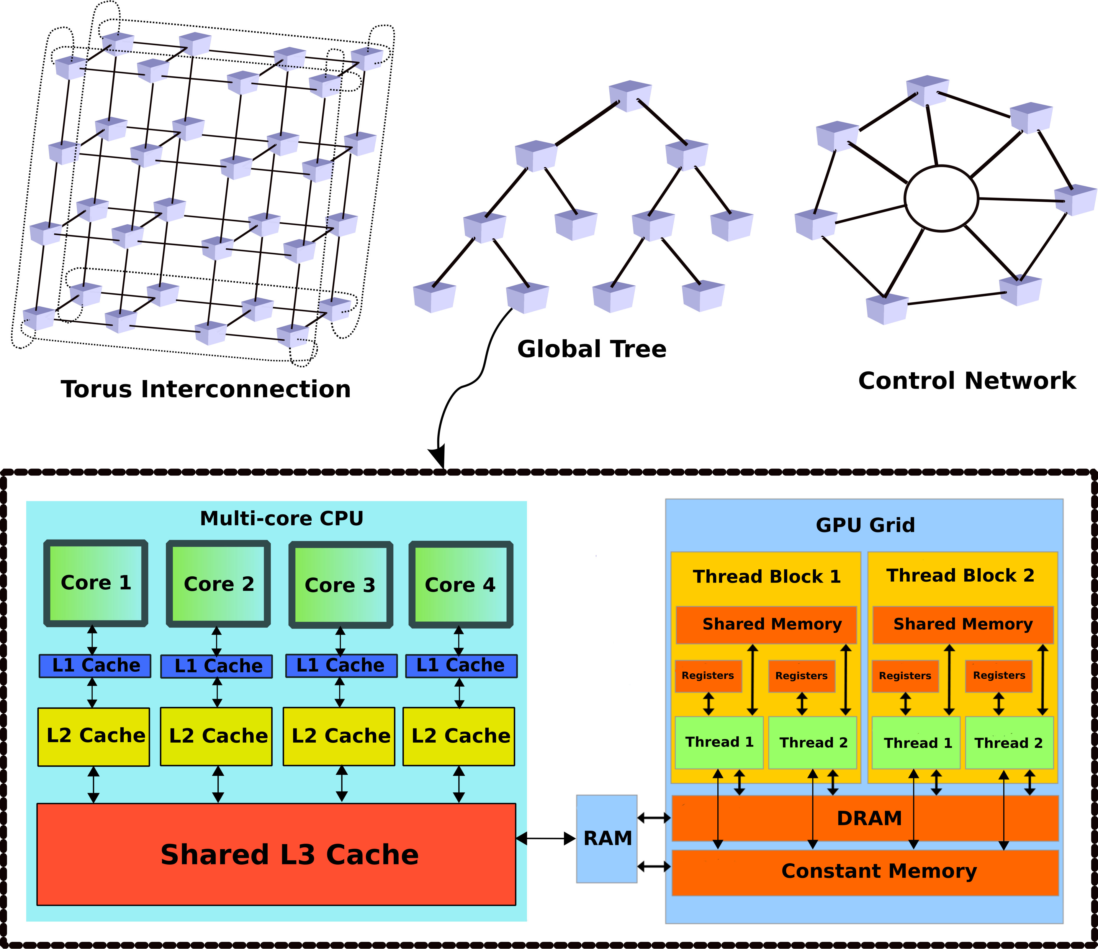 Figure 4
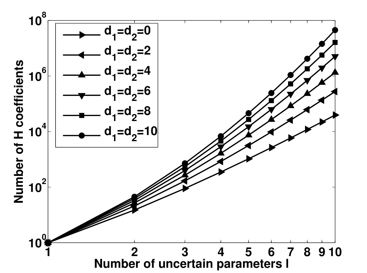 Figure 5
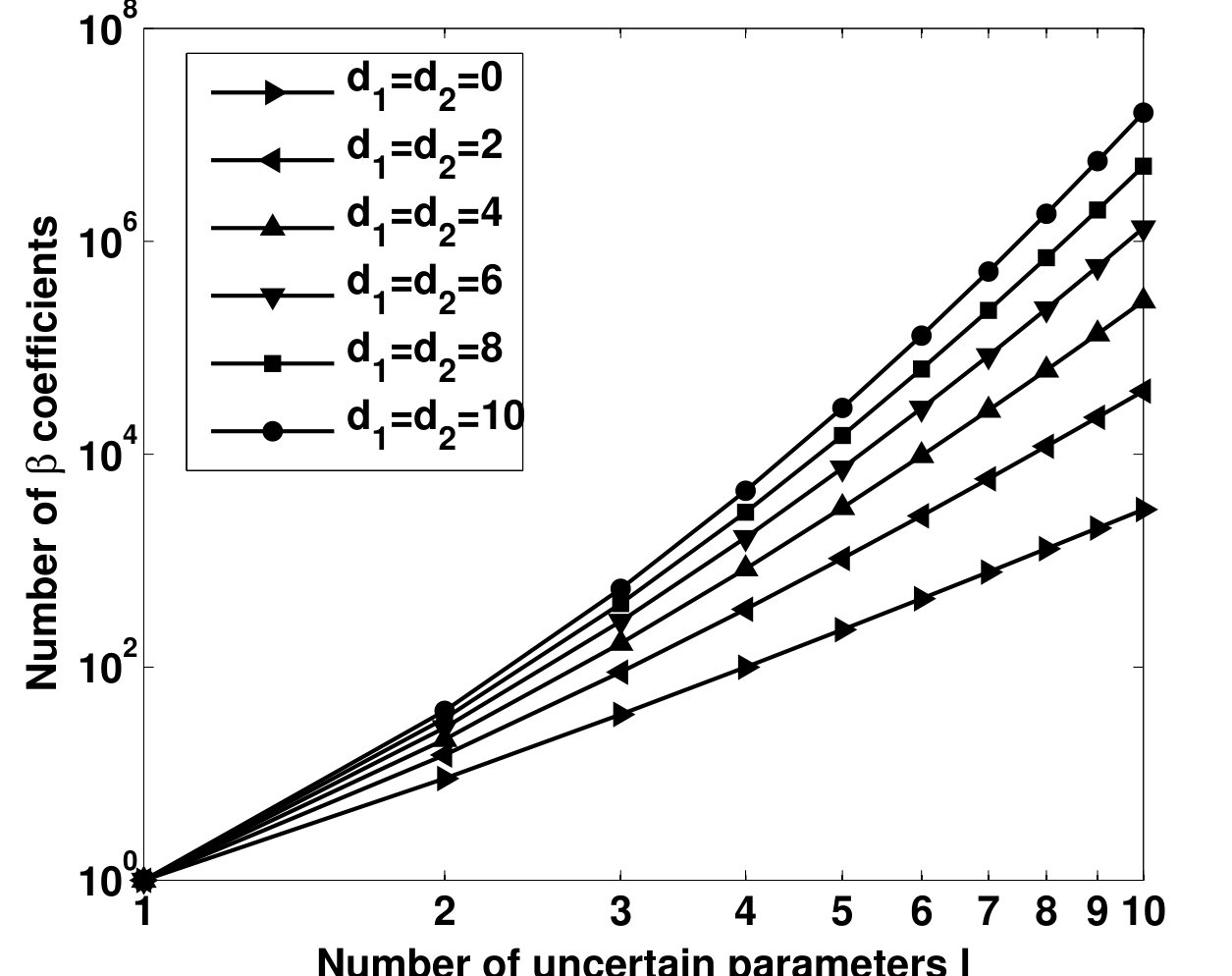 Figure 6
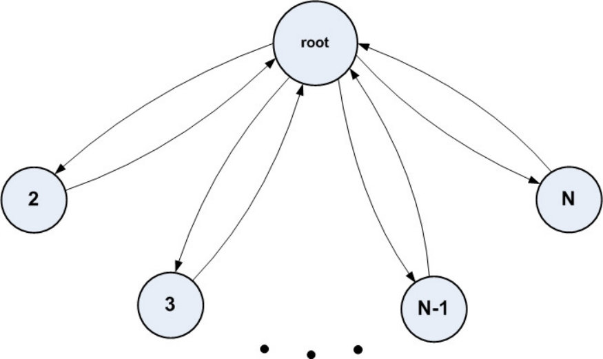 Figure 7
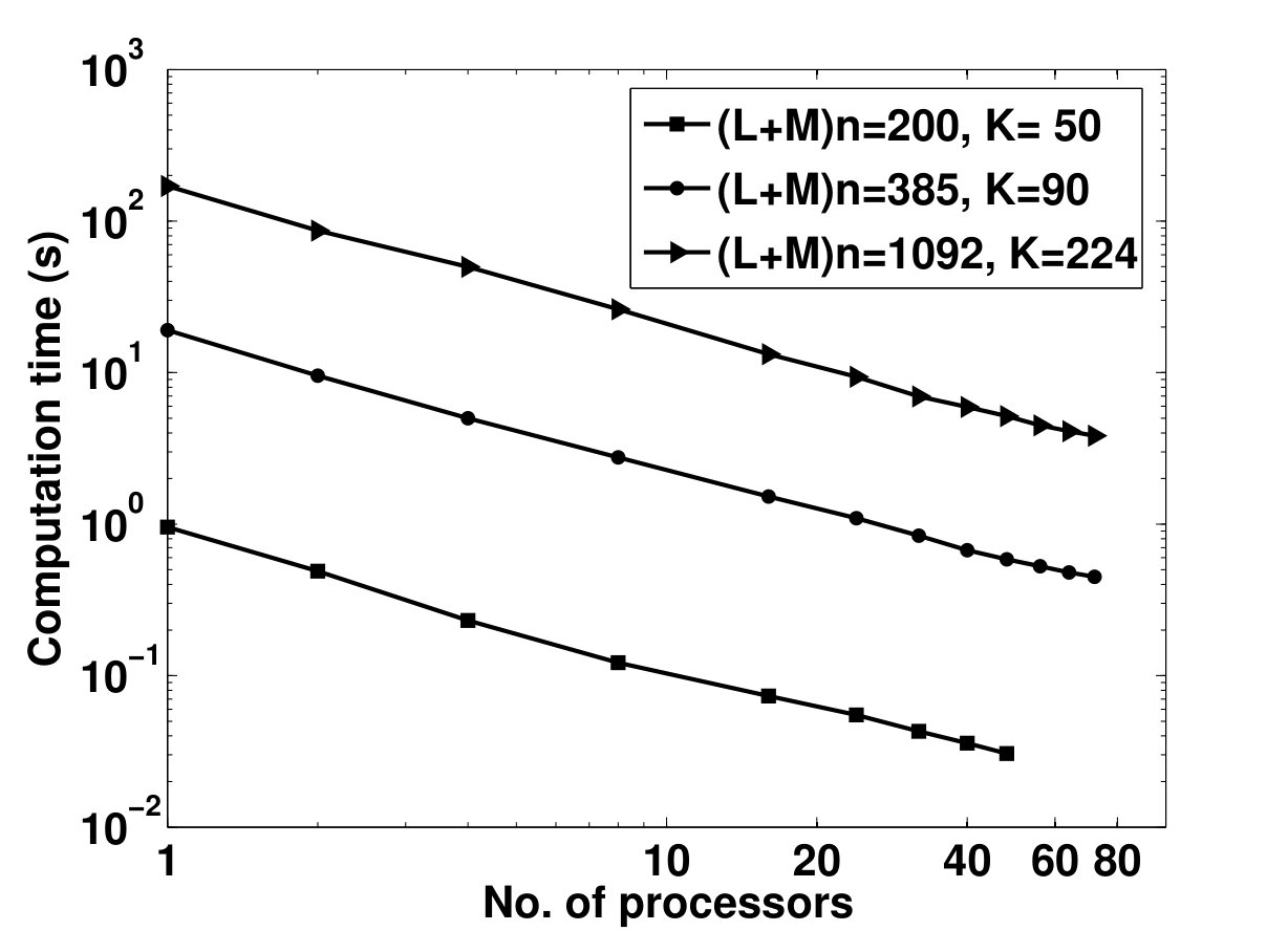 Figure 8
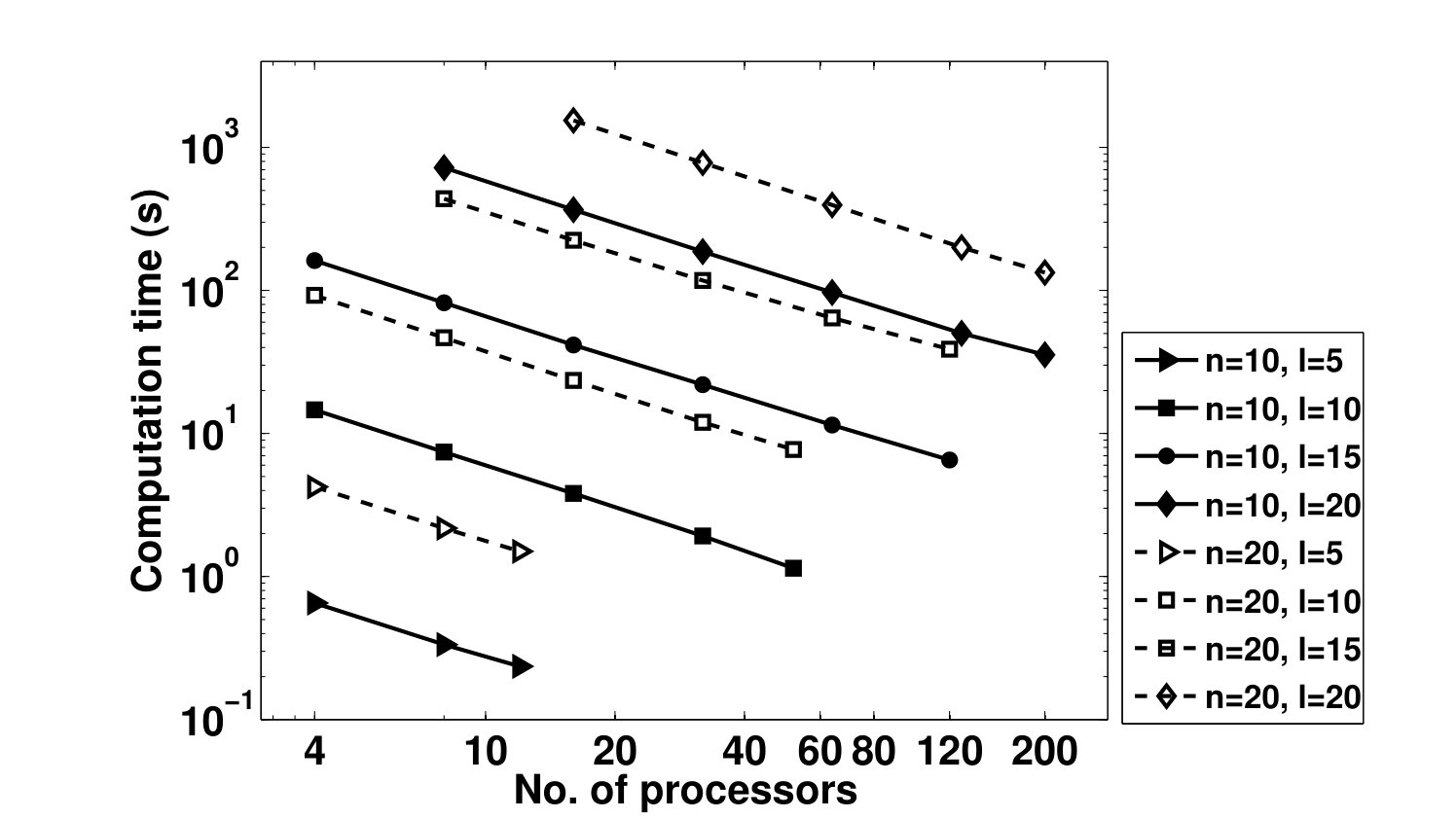 Figure 9
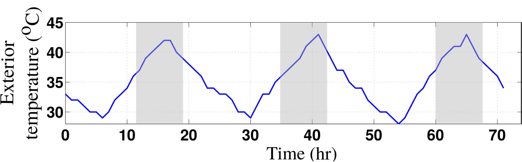 Figure 10
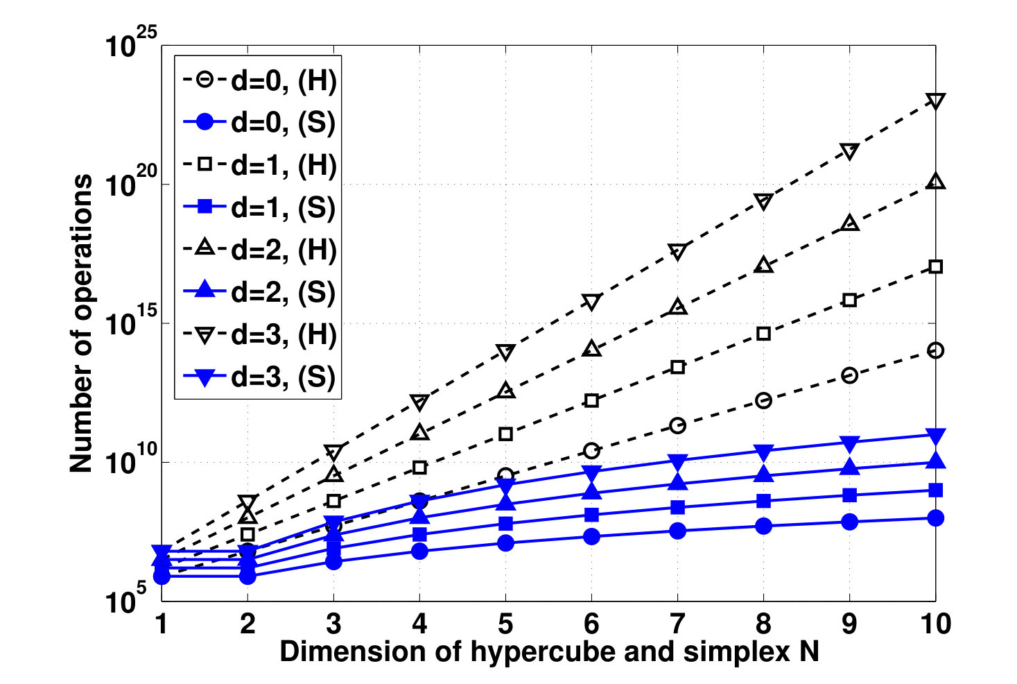 Figure 11
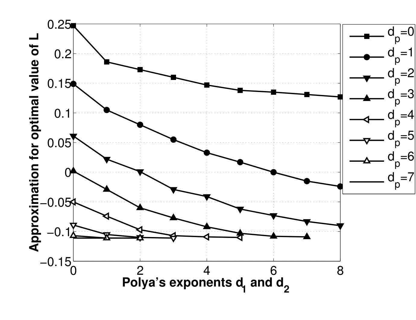 Figure 12
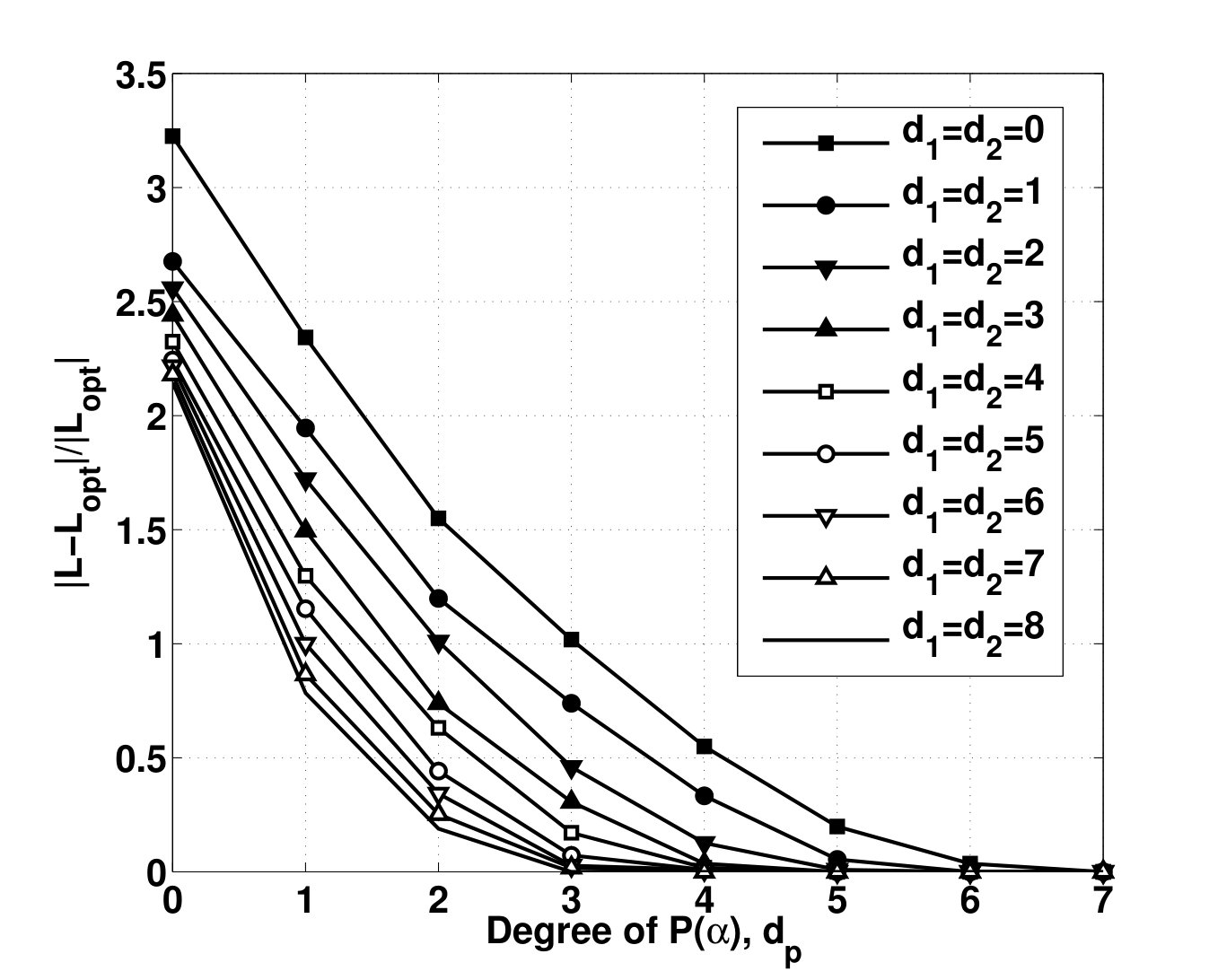 Figure 13
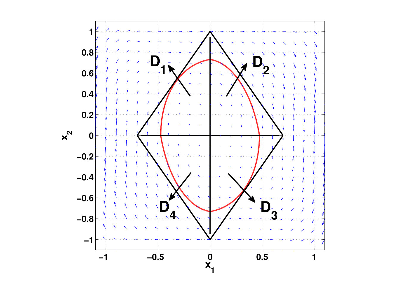 Figure 14
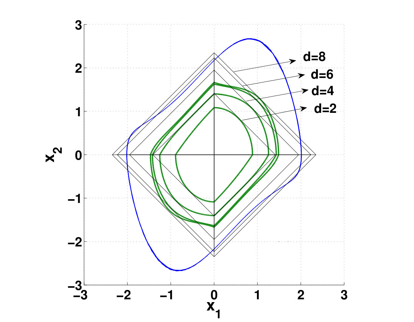 Figure 15
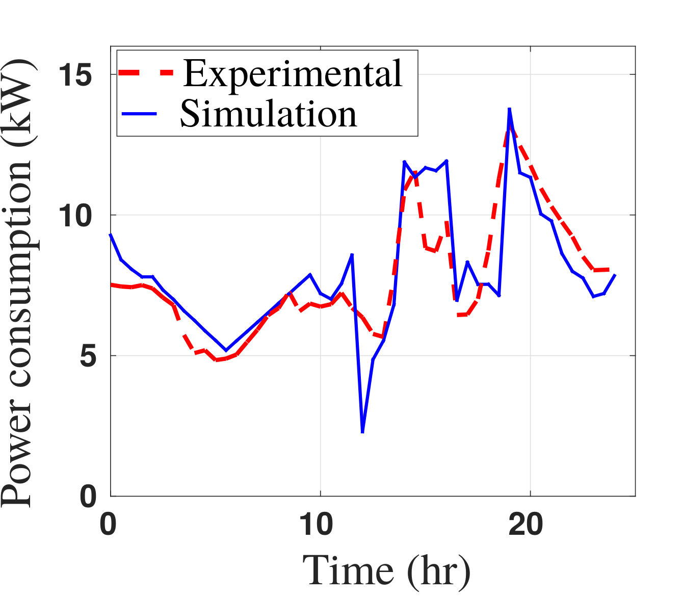 Figure 16
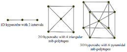 Figure 17
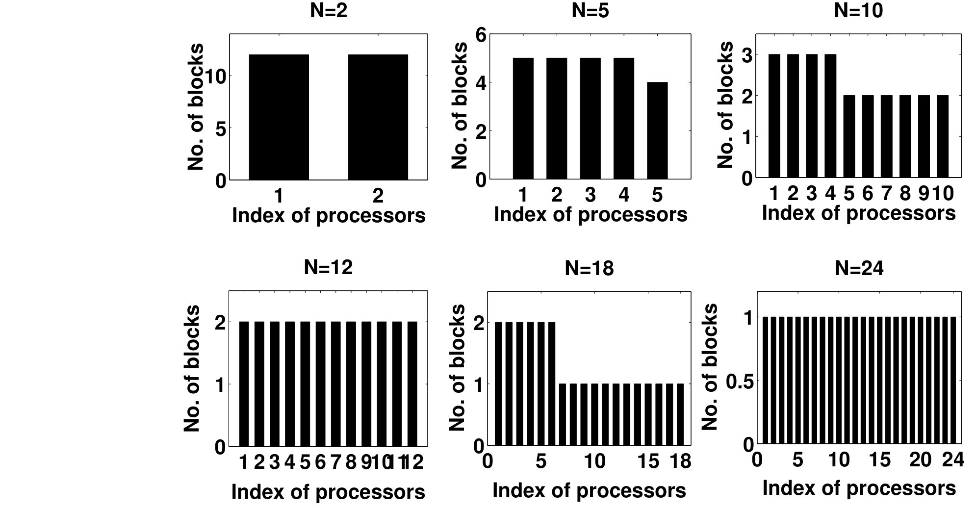 Figure 18
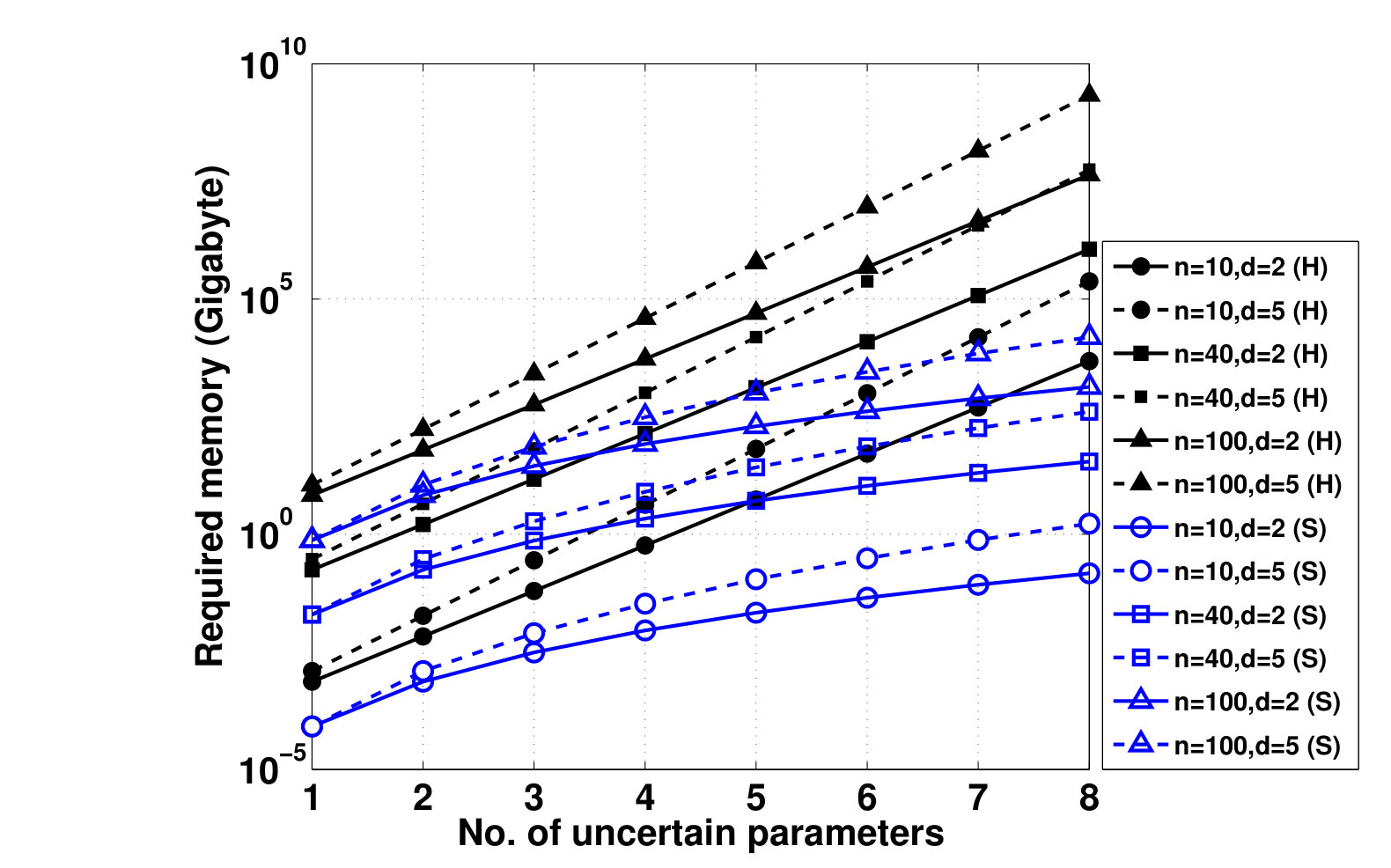 Figure 19
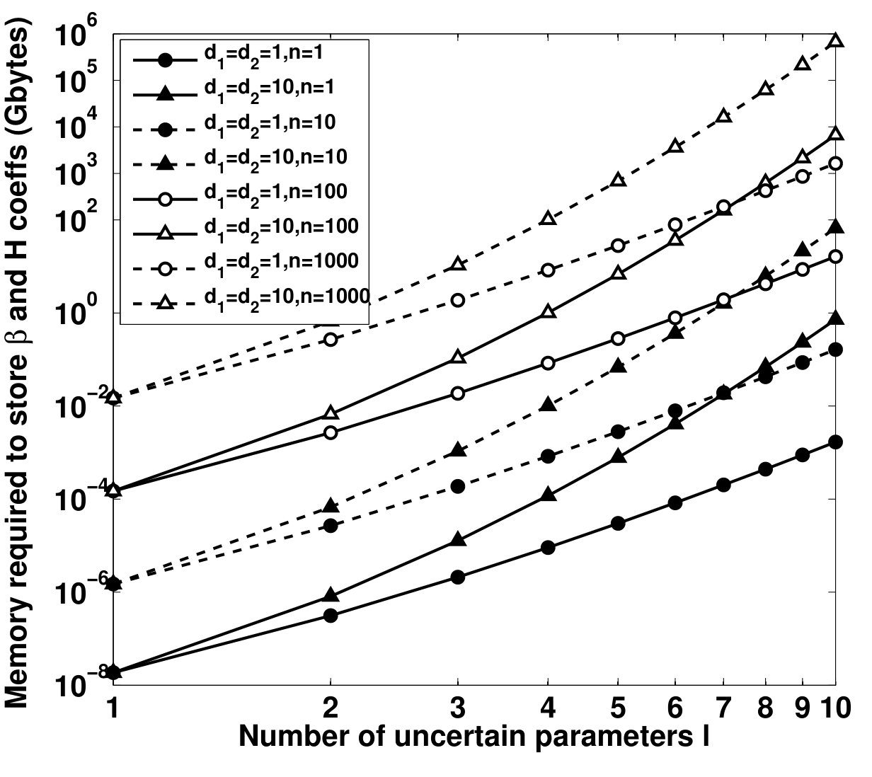 Figure 20
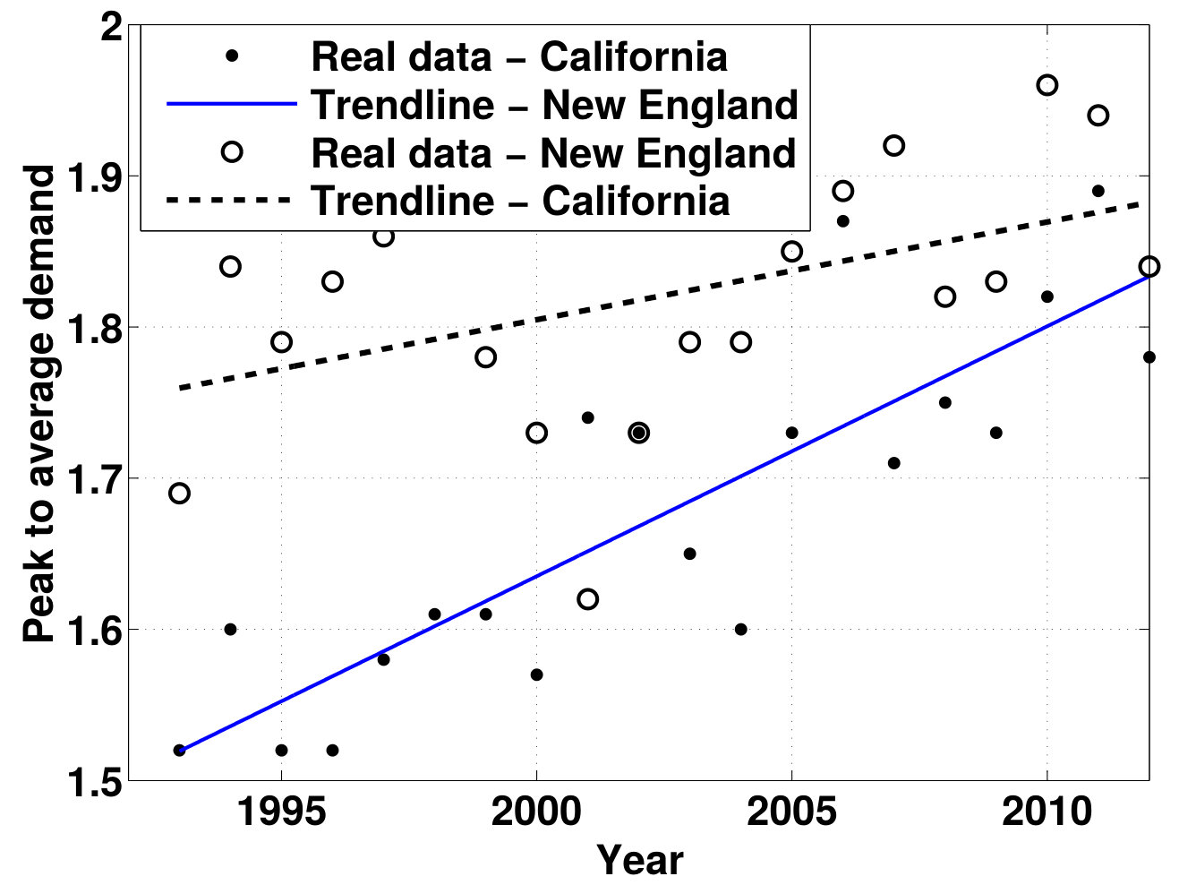 Figure 21
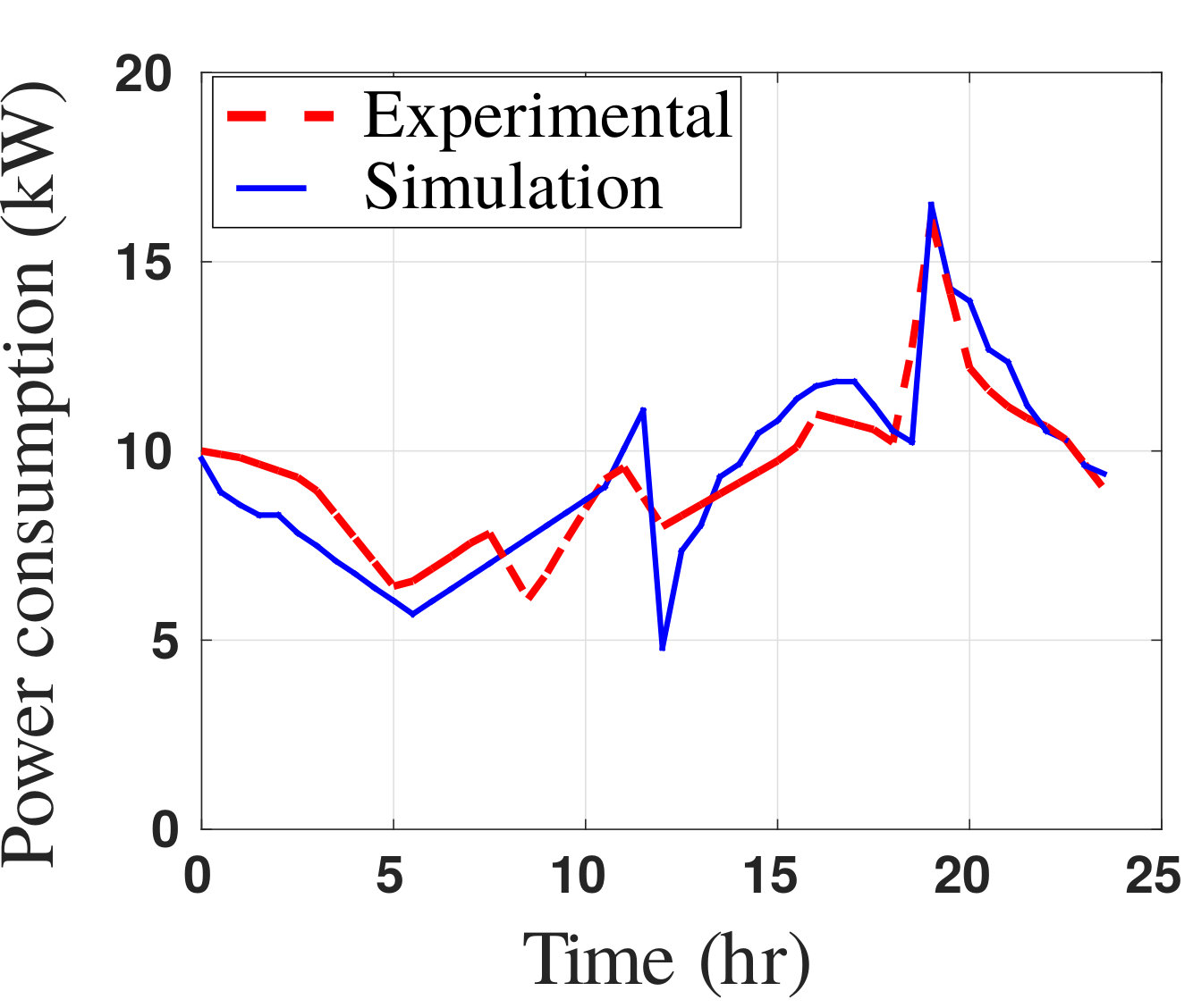 Figure 22
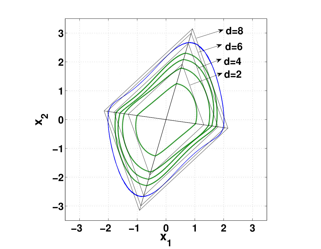 Figure 23
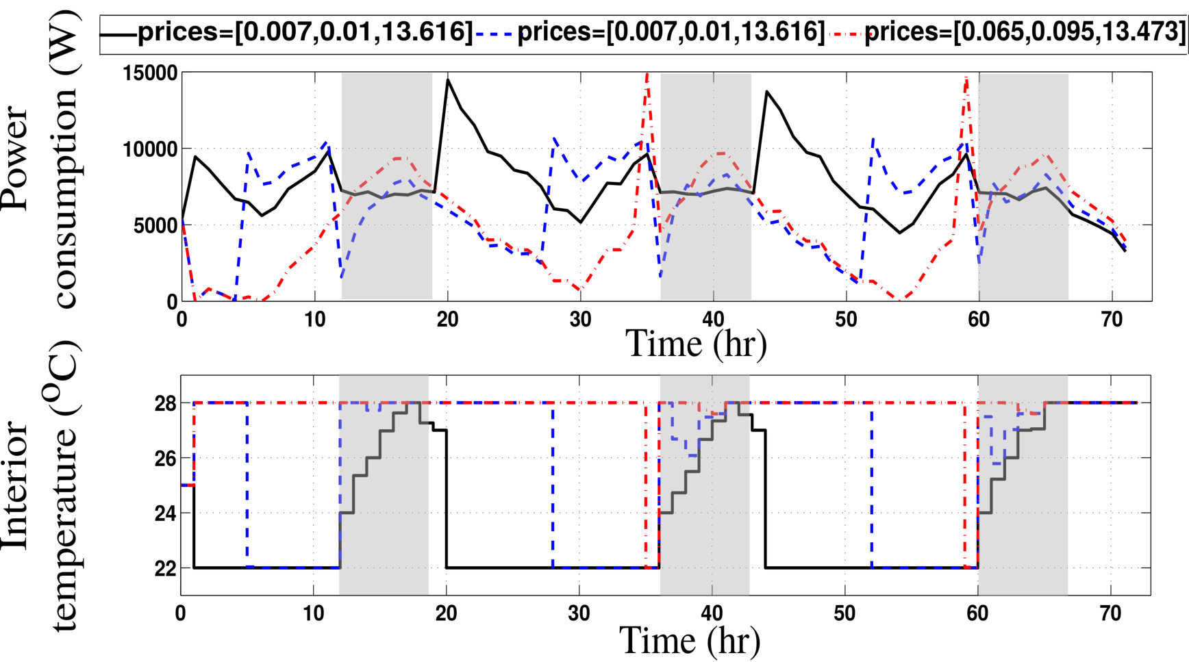 Figure 24
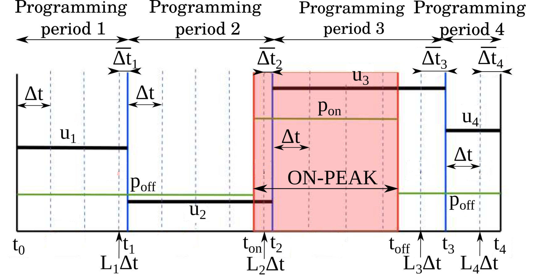 Figure 25
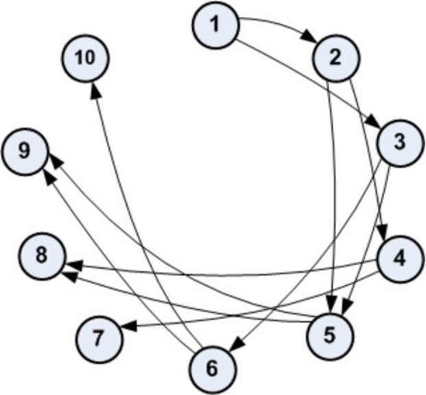 Figure 26
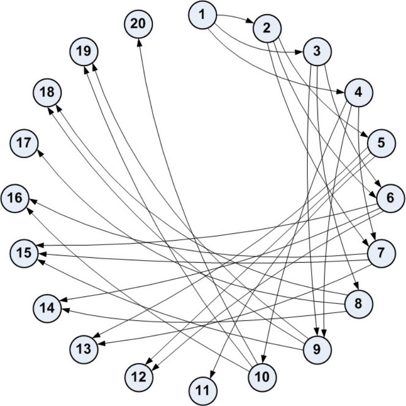 Figure 27
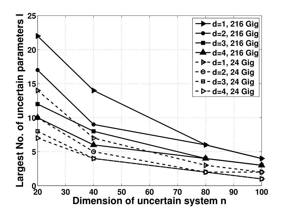 Figure 28
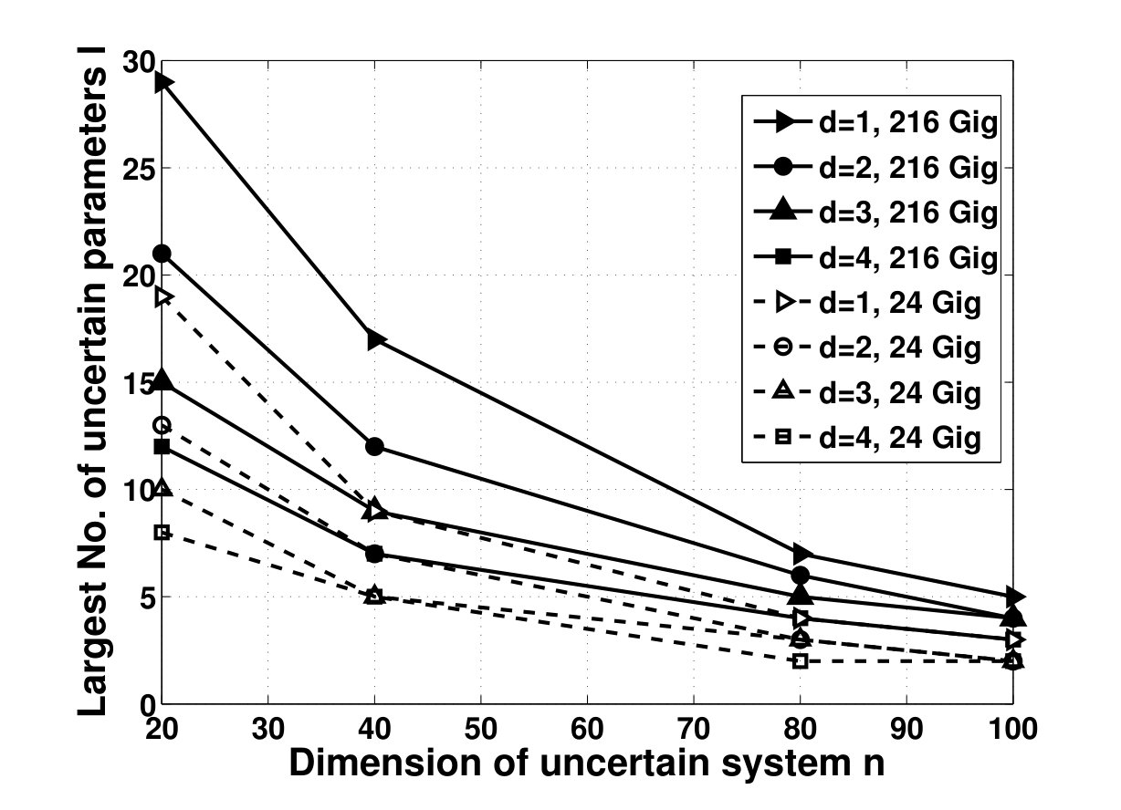 Figure 29
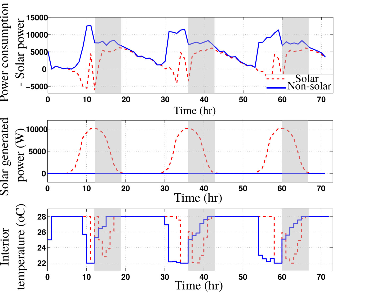 Figure 30
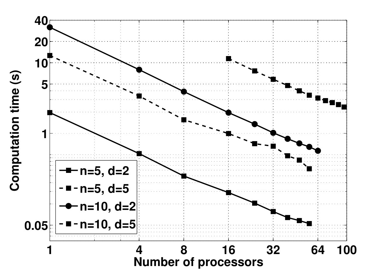 Figure 31
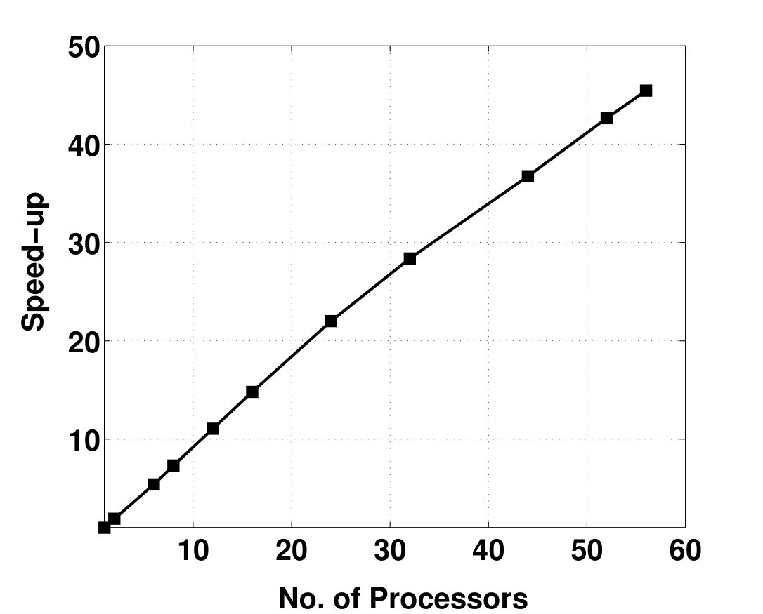 Figure 32
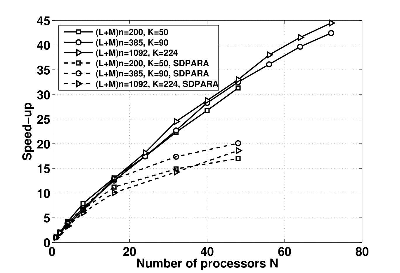 Figure 33
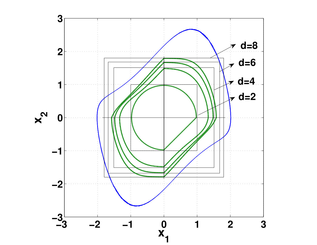 Figure 34
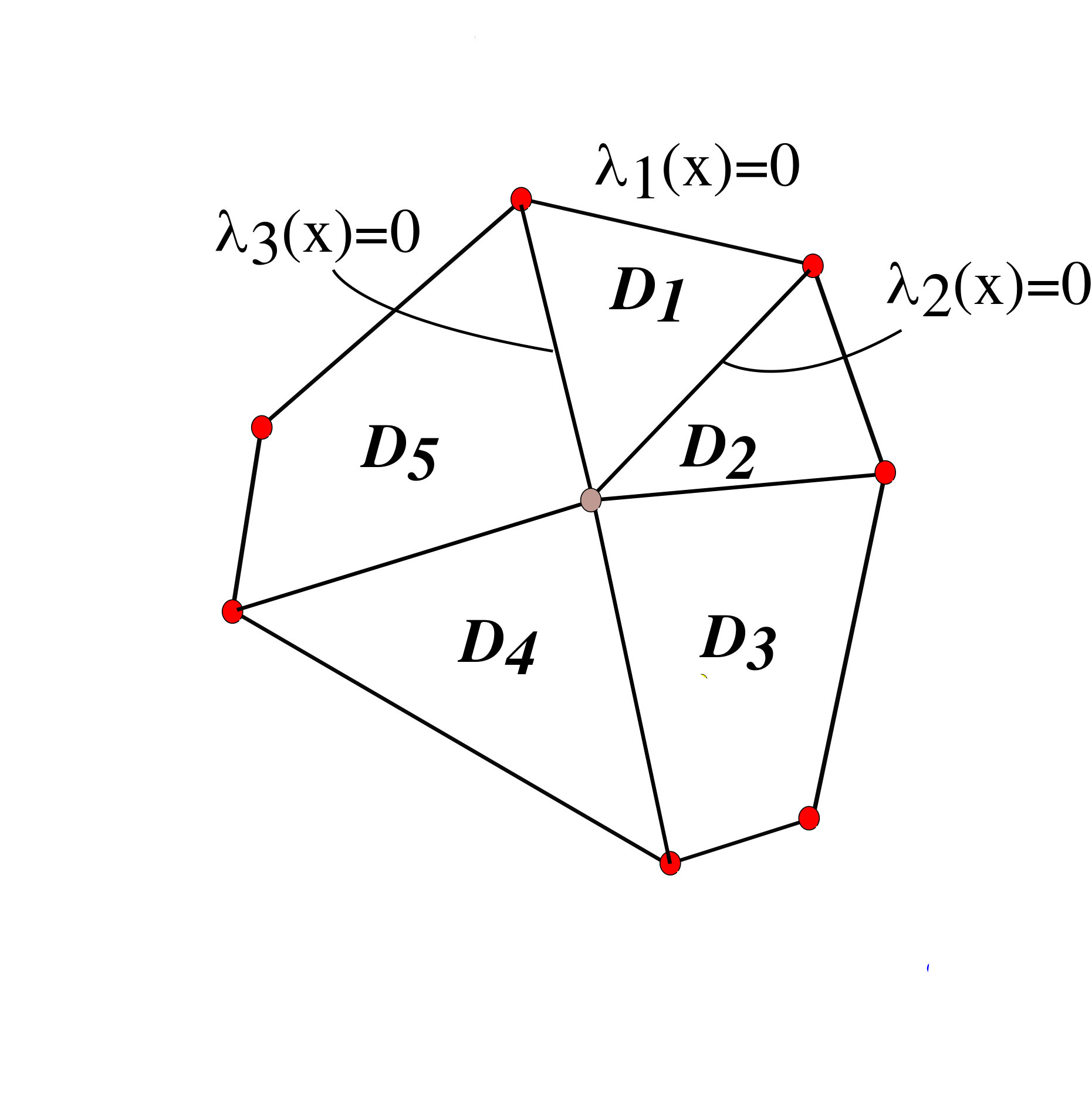 Figure 35
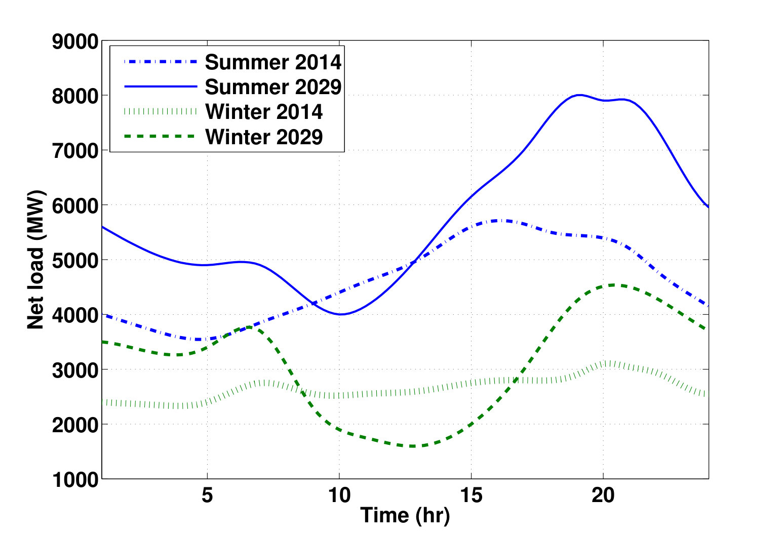 Figure 36
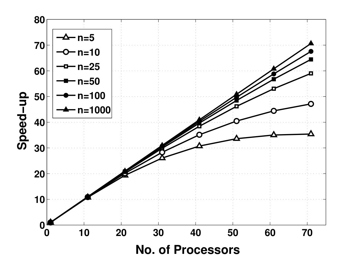 Figure 37
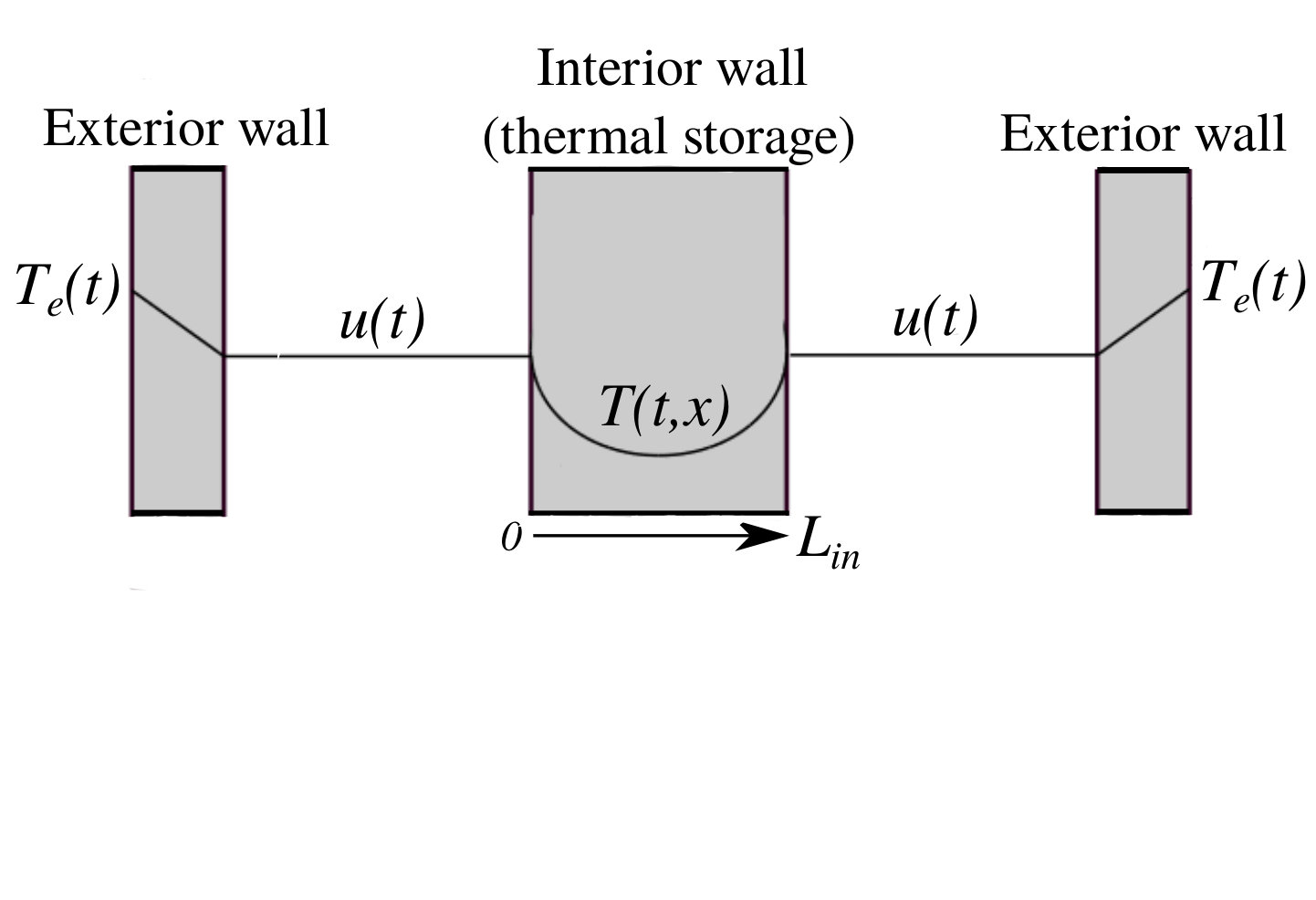 Figure 38
| \pbox60cmNumber of processors | |||
|---|---|---|---|
| \pbox60cmComputational | |||
| cost per processor |
| Number of processors | |||
|---|---|---|---|
| communication cost per processor |
| 0.036 | 0.143 | 0.286 | 0.429 | 0.571 | 0.714 | 0.857 | 0.964 | |
| 0 | 1 | 2 | |
|---|---|---|---|
| 1 | Infeasible | Infeasible | Infeasible |
| 2 | Infeasible | -0.102 | Out of Memory |
| 3 | Infeasible | Out of Memory | Out of Memory |
| 0.4 | 0.0015 | 45 | 0.1 |
| On-peak | Off-peak | Demand | |
|---|---|---|---|
| APS | 0.089 | 0.044 | 13.50 |
| Prices | Demand-limiting | Production cost | Demand peak | |
|---|---|---|---|---|
| high | 46.78 (0.086) | 7.4132 | ||
| Optimal | medium | 51.56 (0.116) | 8.2898 | |
| low | 59.42 (0.168) | 9.6749 |
| Strategy | Production cost | Demand peak | |
|---|---|---|---|
| Optimal | 1,595,309 | 195.607 | |
| SRP | 1,677,516 | 211.79 |
| Customers | Elect. Bill | Demand peak | |
|---|---|---|---|
| Solar & | 50.052 | 6.1947 | |
| Non-solar | 84.717 | 8.6787 | |
| Single Non-solar | 83.333 | 8.3008 | |
| Single Solar | 54.311 | 6.1916 |
Peer Reviews
No public reviews on file for this paper yet. If you reviewed it on a platform where reviews are public (OpenReview, ICLR, NeurIPS, ICML), you can paste yours below so the community can read it here.
Videos
No videos yet. Explain this paper in a talk, walkthrough, or lecture? Add one.
Taxonomy
TopicsAdvanced Optimization Algorithms Research · Stability and Control of Uncertain Systems · Advanced Control Systems Optimization
title
author
Reza Kamyar
Parallel Optimization of Polynomials for Large-scale Problems in
Stability and Control
author
Reza Kamyar
Abstract
In today’s world, optimal operation of ever-growing industries and markets often requires solving optimization problems with unprecedented sizes. Economic dispatch of generating units in power companies, frequency assignment in large mobile communication networks, profit maximization in competitive markets, and optimal operation of smart grids are few examples of many real-world problems which can be closely modeled as optimization over a large number (tens of thousands) of integer- and real-valued decision variables. Unfortunately, majority of the existing commercial off-the-shelf software are not designed to scale to optimization problems of this size. Moreover, in theory, these optimization problems often fall into the class NP-hard - meaning that despite the tremendous effort towards modernization of optimization algorithms, it is widely suspected that no algorithm can find exact solutions to these problems in a reasonable amount of time.
In this thesis, we focus on some of the NP-hard problems in control theory. Thanks to the converse Lyapunov theory, these problems can often be modeled as optimization over polynomials. To avoid the problem of intractability, we establish a trade off between accuracy and complexity. In particular, we develop a sequence of tractable optimization problems - in the form of Linear Programs (LPs) and/or Semi-Definite Programs (SDPs) - whose solutions converge to the exact solution of the NP-hard problem. However, the computational and memory complexity of these LPs and SDPs grow exponentially with the progress of the sequence - meaning that improving the accuracy of the solutions requires solving SDPs with tens of thousands of decision variables and constraints. Setting up and solving such problems is a significant challenge. Unfortunately, the existing optimization algorithms and software are only designed to use desktop computers or small cluster computers - machines which do not have sufficient memory for solving such large SDPs. Moreover, the speed-up of these algorithms does not scale beyond dozens of processors. This in fact is the reason we seek parallel algorithms for setting-up and solving large SDPs on large cluster- and/or super-computers.
We propose parallel algorithms for stability analysis of two classes of systems: 1) Linear systems with a large number of uncertain parameters; 2) Nonlinear systems defined by polynomial vector fields. First, we develop a distributed parallel algorithm which applies Polya’s and/or Handelman’s theorems to some variants of parameter-dependent Lyapunov inequalities with parameters defined over the standard simplex. The result is a sequence of SDPs which possess a block-diagonal structure. We then develop a parallel SDP solver which exploits this structure in order to map the computation, memory and communication to a distributed parallel environment. We produce a Message Passing Interface (MPI) implementation of our parallel algorithms and provide a comprehensive theoretical and experimental analysis on its complexity and scalability. Numerical tests on a supercomputer demonstrate the ability of the algorithm to efficiently utilize hundreds and potentially thousands of processors and analyze systems with 100+ dimensional state-space. We then apply our algorithms to two real-world problems: Stability of plasma in a Tokamak reactor, and optimal electricity pricing in a smart grid environment. Finally, we extend our algorithms to analyze robust stability over more complicated geometries such as hypercubes and arbitrary convex polytopes. Our algorithms can be readily extended to address a wide variety of problems in control; e.g., control synthesis for systems with parametric uncertainty, computing control Lyapunov functions for optimal control problems, and analysis and control of switched/hybrid systems.
TABLE OF CONTENTS
-
3.3 Interior-point Algorithms for Convex Problems with Inequality Constraints
-
3.5 A Primal-dual Interior-point Algorithm for Semi-definite Programming
-
4 PARALLEL ALGORITHMS FOR ROBUST STABILITY ANALYSIS OVER SIMPLEX
-
4.3 Setting-up the Problem of Robust Stability Analysis over a Simplex
-
4.3.3 The Elements of the SDP Problem Associated with Polya’s Theorem
-
4.6.1 Complexity Analysis for Systems with Large Number of States
-
4.6.2 Complexity of Increasing Accuracy/Decreasing Conservativeness
-
4.7.1 Example 1: Application to Control of a Discretized PDE Model in Fusion Research
-
5 PARALLEL ALGORITHMS FOR ROBUST STABILITY ANALYSIS OVER HYPERCUBES
-
5.2 Notation and Preliminaries on Multi-homogeneous Polynomials
-
5.3 Setting-up the Problem of Robust Stability Analysis over Multi-simplex
-
5.3.2 The SDP Elements Associated with the Multi-simplex Version of Polya’s Theorem
-
5.4 Computational Complexity Analysis of the Set-up Algorithm
-
5.4.3 Speed-up and Memory Requirement of the Set-up Algorithm:
-
5.5.2 Example 2: Verifying Robust Stability over a Hypercube
-
6.5.1 Complexity of the LP Associated with Handelman’s Representation
-
6.5.2 Complexity of the SDP Associated with Polya’s Algorithm
-
7 OPTIMIZATION OF SMART GRID OPERATION: OPTIMAL UTILITY PRICING AND DEMAND RESPONSE
-
7.2 Problem Statement: User-level and Utility Level Problems
-
7.3 Solving User- and Utility-level Problems by Dynamic Programming
-
7.4.1 Effect of Electricity Prices on Peak Demand and Production Costs
-
7.4.2 Optimal Thermostat Programming with Optimal Electricity Prices
-
8 SUMMARY, CONCLUSIONS AND FUTURE DIRECTIONS OF OUR RESEARCH
-
8.2.1 A Parallel Algorithm for Nonlinear Stability Analysis Using Polya’s Theorem
-
8.2.2 Parallel Computation for Parameter-varying -optimal Control Synthesis
-
8.2.3 Parallel Computation of Value Functions for Approximate Dynamic Programming
LIST OF TABLES
- 4.1 Per Processor, Per Iteration Computational Complexity of the Set-up Algorithm. is the Number of Monomials Is ; Is the Number of Monomials in ; Is the Number of Monomials in .
- 4.2 Per Processor, Per Iteration Communication Complexity of the Set-up Algorithm. is the Number of Monomials Is ; Is the Number of Monomials in ; Is the Number of Monomials in .
- 4.3 Data for Example 1: Nominal Values of the Plasma Resistivity
- 4.4 Upper Bounds Found for by the SOS Algorithm Using Different Degrees for and (inf: Infeasible, O.M.: Out of Memory)
- 5.1 The Lower-bounds on Computed by Algorithm 7 Using Different Degree Vector and Using Methods in Bliman (2004a) and Chesi (2005).
- 7.1 Building’s Parameters as Determined in Section 7.2.1
- 7.2 On-peak, Off-peak & Demand Prices of Arizona Utility APS
- 7.3 CASE I: Electricity Bills (or Three Days) and Demand Peaks for Different Strategies. Electricity Prices Are from APS.
- 7.4 CASE I: Costs of Production (for Three Days) and Demand Peaks for Various Prices and Strategies. Prices Are Non-regulated and SRP’s Coefficients of Utility Cost Are: 0.00401 \nu=/(MWh)
- 7.5 CASE II: Production Costs (for Three Days) and Demand Peaks Associated with Regulated Optimal Electricity Prices (Calculated by Algorithm 10) and SRP’s Electricity Prices. SRP’s Marginal Costs: a=0.0814\frac{\}{kWh},b=59.76\frac{$}{kW}$
- 7.6 CASE III: Optimal Electricity Prices, Bills (for Three Days) and Demand Peaks for Various Customers. Marginal osts from SRP: a=0.0814\frac{\}{kWh},b=59.76\frac{$}{kW}$
LIST OF FIGURES
- 4.1 Various Interconnections of Nodes in a Cluster Computer (Top), Typical Memory Hierarchies of a GPU and a Multi-core CPU (bottom)
- 4.2 Number of Coefficients vs. the Number of Uncertain Parameters for Different Polya’s Exponents and for
- 4.4 Memory Required to Store the Coefficients and vs. Number of Uncertain Parameters, for Different and
- 4.5 Graph Representation of the Network Communication of the Set-up Algorithm. (a) Communication Directed Graph for the Case . (b) Communication Directed Graph for the Case .
- 4.6 Theoretical Speed-up vs. No. of Processors for Different System Dimensions for , , and , Where
- 4.7 The Number of Blocks of the SDP Elements Assigned to Each Processor. An Illustration of Load Balancing.
- 4.8 The Communication Graph of the SDP Algorithm
- 4.9 Speed-up of Set-up and SDP Algorithms vs. Number of Processors for a Discretized Model of Magnetic Flux in Tokamak
- 4.10 Upper Bound on Optimal vs. Polya’s Exponents and , for Different Degrees of . ().
- 4.12 Computation Time of the Parallel Set-up Algorithm vs. Number of Processors for Different Dimensions of Linear System and Numbers of Uncertain Parameters - Executed on Blue Gene Supercomputer of Argonne National Labratory
- 4.13 Computation Time of the Parallel SDP Algorithm vs. Number of Processors for Different Dimensions of Primal Variable and of Dual Variable - Executed on Karlin Cluster Computer
- 4.14 Comparison Between the Speed-up of the Present SDP Solver and SDPARA 7.3.1, Executed on Karlin Cluster Computer
- 4.15 Largest Number of Uncertain Parameters of -Dimensional Systems for Which the Set-up Algorithm (Left) and SDP Solver (Right) Can Solve the Robust Stability Problem of the System Using 24 and 216 GB of RAM
- 5.1 Number of Operations vs. Dimension of the Hypercube, for Different Polya’s Exponents . (H): Hypercube and (S): Simplex.
- 5.2 Required Memory for the Calculation of SDP Elements vs. Number of Uncertain Parameters in Hypercube and Simplex, for Different State-space Dimensions and Polya’s Exponents . (H): Hypercube, (S): Simplex.
- 5.3 Execution Time of the Set-up Algorithm vs. Number of Processors, for Different State-space Dimensions and Polya’s Exponents
- 6.1 An Illustration of a D-decomposition of a 2D Polytope. for .
- 6.2 Decomposition of the Hypercube in , and Dimensions
- 6.3 Number of Decision Variables and Constraints of the Optimization Problems Associated with Algorithm 1, Polya’s Algorithm and SOS Algorithm for Different Degrees of the Lyapunov Function and the Vector Field
- 6.4 The Largest Level-set of Lyapunov Function (6.21) Inscribed in Polytope (6.20)
- 6.5 Largest Level-sets of Lyapunov Functions of Different Degrees and Their Associated Parallelograms
- 7.1 Effect of Solar Power on Demand: Net Loads for Typical Summer and Winter Days in Arizona in 2014 and for 2029 (Projected), from Arizona Public Service (2014)
- 7.2 Peak to Average Demand of Electricity and Its Trend-line in California and New England from 1993 to 2012, Data Adopted from Shear (2014)
- 7.3 A Schematic View of Our Thermal Mass Model
- 7.4 Simulated and Measured Power Consumptions
- 7.5 An Illustration for the Programming Periods of the 4-Setpoint Thermostat Problem, Switching Times , Pricing Function , and .
- 7.6 External Temperature of Three Typical Summer Days in Phoenix, Arizona. Shaded Areas Correspond to On-peak Hours.
- 7.7 CASE I: Power Consumption and Temperature Settings for Various Programming Strategies Using APS’s Rates.
- 7.8 CASE I: Power Consumption and Optimal Temperature Settings for High, Medium and Low Demand Penalties. Shaded Areas Correspond to On-peak Hours.
- 7.9 CASE I: Power Consumption and Temperature Settings for High, Medium and Low Demand Penalties Using 4-Setpoint Thermostat Programming.
- 7.10 CASE III: Power Consumption, Solar Generated Power and Optimal Temperature Settings for the Non-solar and Solar Users.
Chapter 1 INTRODUCTION
Consider problems such as portfolio optimization, path-planning, structural design, local stability of nonlinear ordinary differential equations, control of time-delay systems and control of systems with uncertainties. These problems can all be formulated as polynomial optimization and/or optimization of polynomials. In this dissertation, we show how computation can be applied in a variety of ways to solve these classes of problems. A simple example of polynomial optimization is , where is a multi-variate polynomial and . In general, since and are not convex, this is not a convex optimization problem. In fact, it has been proved that polynomial optimization is NP-hard (L. Blum and Smale (1998)). Fortunately, algorithms such as branch-and-bound can find arbitrarily precise solutions to polynomial optimization problems by repeatedly partitioning into subsets and computing lower and upper bounds on over each . To find an upper bound for over each , one could use a local optimization algorithm such as sequential quadratic programming. To find a lower bound on over each , one can solve the following optimization problem.
[TABLE]
This problem is in fact an instance of the problem of optimization of polynomials. Optimization of polynomials is convex, yet again NP-hard. We will discuss optimization of polynomials in more depth in Chapter 2. In the following, we discuss some of the state-of-the-art methods for solving optimization of polynomials - hence finding lower bounds on .
1.1 Sum of Squares Method
One approach to find lower bounds on the optimal objective is to apply Sum of Squares (SOS) programming (Parrilo (2000), Papachristodoulou et al. (2013)). A polynomial is SOS if there exist polynomials such that . The set is called an SOS decomposition of , where is the ring of real polynomials. An SOS program is an optimization problem of the form
[TABLE]
where and are given. If is SOS, then clearly on . While verifying on is NP-hard, verifying whether is SOS - hence non-negative - can be done in polynomial time (Parrilo (2000)). It was first shown in Parrilo (2000) that verifying the existence of a SOS decomposition is a Semi-Definite Program (SDP). Fortunately, there exist several algorithms (Monteiro (1997); Helmberg et al. (1996); Alizadeh et al. (1998)) and solvers (Yamashita et al. (2010); Sturm (1999); Tutuncu et al. (2003)) which solve SDPs to arbitrary precision in polynomial time. To find lower bounds on , consider the SOS program
[TABLE]
Clearly . One can compute by performing a bisection search on and using semi-definite programming to verify is SOS. SOS programming can also be used to find lower bounds on global minimum of polynomials over a semi-algebraic set generated by . Given Problem (1.1) with , Positivstellensatz results (Stengle (1974), Putinar (1993), Schmudgen (1991)) define a sequence of SOS programs whose objective values form a sequence of lower bounds on the global minimum . For instance, Putinar’s Positivstellensatz defines the optimization problem
[TABLE]
where denotes the cone of SOS polynomials of degree . Putinar (1993) has shown that under certain conditions (verifiable by semi-definite programming) on and for sufficiently large , . See Laurent (2009) for a comprehensive discussion on the Positivstellensatz results.
1.2 Moments Method
As a dual to SOS program, Lasserre (2001) used the theory of moments to define a sequence of lower bounds for global optima of polynomials. Let , where is compact and with the index set . Let us denote the degree of by . Then, Lasserre (2001) showed that defined as
[TABLE]
is a lower bound on . In Equation (1.4), , where is called the moment of order and is represented by any probability measure111Let be a set and be a algebra over . Then is a probability measure if
and .
For all countable collections of pairwise disjoint subsets of , .
on such that . Moreover, is called the moment matrix associated with sequence and in two dimensions is defined as
[TABLE]
It can be shown that the SDPs in (1.4) are duals to the SDPs in (1.3) - implying that . Indeed, if has a non-empty interior, then for all sufficiently large , the duality gap is zero, i.e., . See Laurent (2009) and Jeyakumar et al. (2014) for conditions on convergence of the lower bounds to global minima and extension of moments method to polynomial optimization over non-compact semi-algebraic sets.
In the sequel, we explore the merits of some of the alternatives to SOS programming and moments method. There exist several results in the literature that can be applied to polynomial optimization; e.g., Quantifier Elimination (QE) algorithms (Collins and Hoon (1991)) for testing the feasibility of semi-algebraic sets, Reformulation Linear Techniques (RLTs) (Sherali and Tuncbilek (1992, 1997)) for linearizing polynomial optimizations, Polya’s theorem (G. Hardy and Polya (1934)) for positivity over the positive orthant, Bernstein’s (Boudaoud et al. (2008); Leroy (2012)) and Handelman’s (Handelman (1988a)) theorems for positivity over simplices and convex polytopes, and other results based on Groebner bases (Adams and Loustaunau (1994)) and Blossoming (Ramshaw (1987)) techniques. In particular, we will focus on Polya’s, Bernstein’s and Handelman’s results in more depth and elaborate on the computational advantages of these results over the others. The discussion of the other results are beyond the scope of this dissertation, however the ideas behind these results can be summarized as follows.
1.3 Quantifier Elimination
QE algorithms apply to First-Order Logic formulae, e.g.,
[TABLE]
to eliminate the quantified variables and (preceded by quantifiers ) and construct an equivalent formula in terms of the unquantified variable . The key result underlying QE algorithms is Tarski-Seidenberg theorem (Tarski (1951)). The theorem implies that for every formula of the form , where , there exists an equivalent quantifier-free formula of the form with . QE implementations (e.g., Brown (2003) and Dolzmann and Sturm (1997)) with a bisection search yields the exact solution to optimization of polynomials, however the complexity scales double exponentially in the dimension of variables .
1.4 Reformulation Linear Techniques
RLT was initially developed to find the convex hull of feasible solutions of zero-one linear programs (Sherali and Adams (1990)). It was later generalized by Sherali and Tuncbilek (1992) to address polynomial optimizations of the form subject to . RLT constructs a hierarchy of linear programs by performing two steps. In the first step (reformulation), RLT introduces the new constraints for all . In the second step (linearization), RTL defines a linear program by replacing every product of variables by a new variable. By increasing and repeating the two steps, one can construct a hierarchy of lower bounding linear programs. A combination of RLT and branch-and-bound partitioning of was developed by Sherali and Tuncbilek (1997) to achieve tighter lower bounds on the global minimum. For a survey of different extensions of RLT see Sherali and Liberti (2009).
1.5 Groebner Basis Technique
Groebner bases can be used to reduce a polynomial optimization over a semi-algebraic set to the problem of finding the roots of univariate polynomials (Chang and Wah (1994)). First, one needs to construct the system of polynomial equations
[TABLE]
where is the Lagrangian function. It is well-known that the set of solutions to (1.5) is the set of extrema of the polynomial optimization . Let
[TABLE]
Using the elimination property (Adams and Loustaunau (1994)) of the Groebner bases, the minimal Groebner basis of the ideal of defines a triangular-form system of polynomial equations. This system can be solved by calculating one variable at a time and back-substituting into other polynomials. The most computationally expensive part is the calculation of the Groebner basis, which in the worst case scales double-exponentially in the number of decision variables.
1.6 Blossoming Technique
The blossoming technique involves a bijective map between the space of polynomials and the space of multi-affine functions (polynomials that are affine in each variable), where is the degree of in variable . For instance, the blossom of a cubic polynomial is the multi-affine function
[TABLE]
It can be shown that the blossom, , of any polynomial with degree in variable satisfies the so-called diagonal property (Ramshaw (1987)), i.e.,
[TABLE]
By using this property, one can reformulate any polynomial optimization as
[TABLE]
where and is the semi-algebraic set defined by the blossoms of the generating polynomials of . In the special case, where is a hypercube, Sassi and Girard (2012) showed that the Lagrangian dual optimization problem to Problem (1.6) is a linear program. Hence, the optimal objective value of this linear program is a lower bound on the minimum of over the hypercube. Application of blossoming in estimation of reachability sets of discrete-time dynamical systems can be found in Sassi et al. (2012).
1.7 Bernstein, Polya and Handelman Theorems
While QE, RLT, Groebner bases and blossoming are all useful techniques with advantages and disadvantages (such as exponential complexity), we focus on Polya’s, Bernstein’s and Handelman’s theorems - results which yield polynomial-time tests for positivity of polynomials. Polya’s theorem yields a basis to represent the cone of polynomials that are positive over the positive orthant. Bernstein’s and Handelman’s theorems yield bases which represent the cones of polynomials that are positive over simplices and convex polytopes, respectively. Similar to SOS programming, one can find certificates of positivity using Polya’s, Bernstein’s and Handelman’s representations by solving a sequence of Linear Programs (LPs) and/or SDPs. However, unlike the SDPs associated with SOS programming, the SDPs associated with these theorems have a block-diagonal structure. In this dissertation, we exploit this structure to design parallel algorithms for optimization of polynomials of high degrees with several independent variables. See Kamyar and Peet (2012a), Kamyar and Peet (2012b), Kamyar and Peet (2013) and Kamyar et al. (2013) for parallel implementations of variants of Polya’s theorem applied to various Lyapunov inequalities.
Unfortunately, unlike the SOS methodology, the bases given by Polya’s theorem, Bernstein’s theorem and Handelman’s theorem cannot be used to represent the cone of non-negative polynomials which have zeros in the interior of simplices and polytopes. This is indeed a barrier against using these theorems to compute polynomial Lyapunov functions, since Lyapunov functions, by definition, have a zero at the origin. There do, however, exist some variants of Polya’s theorem which consider zeros at the corners Powers and Reznick (2006) and edges Castle et al. (2011) by constructing local certificates of non-negativity over closed subsets, , of the simplex such that is the simplex. These results apply to non-negative polynomials whose zeros are on the corners and/or edges of the simplex. Moreover, Oliveira et al. (2008) and Kamyar and Peet (2012b) propose versions of Polya’s theorem which prove positivity over hypercubes by: 1) Providing certificates of positivity on the Cartesian product of unit simplices; and 2) Introducing a one-to-one map between products of unit simplices (multi-simplex) and hypercubes. A generalization of Polya’s theorem for proving positivity on the entire was introduced by de Loera and Santos (1996). This generalization first applies Polya’s theorem to each orthant of to compute a certificate of positivity over each orthant. Then, it uses the merging technique in Lombardi (1991) to obtain a unified certificate - in the form of SOS of rationals - over . A recent extension of Polya’s theorem by Dickinson and Pohv (2014) can be used to prove positivity over an intersection of a semi-algebraic set with the positive orthant. Finally, positivity of polynomials with rational exponents can be verified by a weak version of Polya’s theorem in Delzell (2008).
1.8 Motivations and Summary of Contributions
The novelty of our research centers on the areas of: computation and energy. In the realm of computation, we observed that processors speeds are not growing at the rate they once were. The entire controls community seems to have ignored this fact, since everyone speaks of polynomial-time algorithms as the gold standard for what the solution to a control problem should look like. But what good is a polynomial-time algorithm when the degree of the polynomial is bounded by the current state-of-the-art computers. Our solution was to look at the only area where the computing world was getting faster (growing) - supercomputers. Surprisingly, there have been no studies on the use of parallel computers for controls since the 1970’s. The reason was that the mathematical machinery for analysis and control is based on Semidefinite Programming, which is inherently sequential (NC-hard). Our idea, however, was that if the SDP problem has special structure, then this structure can be exploited to distribute computation among processors. With this in mind, we decided to seek out alternatives to the classical Sum-of-Squares approach to nonlinear and robust stability analyses. We identified more than seven different alternatives to the Sum-of-Squares approach. In the end, not all of these had usable structures for parallelization. However, we identified three which did: polynomial positivity results by Handelman, Polya and Bernstein. To demonstrate how well this approach works in practice, we developed a Message Passing Interface code for Polya’s theorem. The result enabled stability analysis for systems three times larger (in terms of number of states) than any other algorithm. As a real-world application, we further used our code to analyze robust stability of plasma in the Tore Supra Tokamak reactor.
In the realm of energy, we noticed that the two electrical utility companies of Arizona (APS and SRP) have recently started charging their customers for their maximum rate of electricity usage. This intrigued us as a mathematical problem of how to optimize the thermostat settings of HVAC systems (the major sources of electricity consumption in Arizona) in order to minimize the electricity bill. This problem is interesting in that the time of peak electricity use is not usually at the hottest time of day, but rather a couple of hours after - a behaviour which is usually associated with a diffusion PDE. We used the heat equation to model the thermostat programming problem as an optimal control problem and it turned out to be unsolved. The mathematical reason being that the cost function is not separable in time - a property which is necessary for optimal control algorithms to converge to an optimal solution. We noticed that an arbitrarily precise approximation of the cost function however, satisfy certain properties which make it solvable on a Pareto-optimal front. The result is an optimal thermostat which can significantly reduce the electricity bills and peak demand of both solar and nonsolar customers under the current pricing plans. Expanding this approach, we started thinking about related topics, such as how to set the demand price on order to influence customers’ behavior in an optimal manner. Based on that, we proposed an optimal pricing algorithm which resulted in a moderate reduction in the cost of generating, transmission and distribution of electricity at SRP.
We highlight our contributions as follows. In Chapter 4, we propose a parallel set-up algorithm which applies Polya’s theorem to the parameter-dependent Lyapunov inequalities and with belonging to the standard simplex. Feasibility of these inequalities implies robust stability of the system of linear Ordinary Differential Equations (ODEs) over the simplex. The output of our set-up algorithm is a sequence of SDPs of increasing size and precision. A solution to any of these SDPs yield a Lyapunov function which is quadratic in the states and depends polynomially on the uncertain parameters. An interesting property of these SDPs is that they possess a block-diagonal structure. We show how this structure can be exploited to design a parallel interior-point primal-dual SDP solver which distributes the computation of search direction among a large number of processors. We then produce a Message Passing Interface (MPI) implementation of our set-up and solver algorithms. Through numerical experiments, we show that these algorithms achieve a near-linear theoretical and experimental speed-up (the increase in processing speed per additional processor). Moreover, our numerical experiments on cluster computers demonstrate the ability of our algorithms in utilizing hundreds and potentially thousands of processors to analyze systems with 100+ states.
In Chapter 5, we generalize our methodology to perform robust stability analysis over hypercubes. We first propose an extended version of Polya’s theorem. This theorem parameterizes every homogeneous polynomial which is positive over a hypercube. We then propose an extended set-up algorithm which maps the computation and memory - associated with applying the extended Polya’s theorem to stability analysis problems - to parallel machines. This set-up algorithm has no centralized computation and its per-core communication complexity scales polynomially with the state-space dimension and the number of uncertain parameters. As the result, it demonstrates a near-linear speed-up.
In Chapter 6, we further extend our analysis to address stability of nonlinear ODEs defined by a polynomial vector field . Our proposed solution to this problem is to reformulate the nonlinear stability problem using only strictly positive forms. Specifically, we use our extended version of Polya’s theorem in Chapter 5 to compute a matrix-valued homogeneous polynomial such that and for all inside a hypercube containing the origin in its interior. This yields a Lyapunov function of the form for the system . To do this, we design a new parallel set-up algorithm which applies Polya’s theorem to the inequalities and . The result is a sequence of SDPs with coefficients of as decision variables. Again, we show that these SDPs have a block-diagonal structure - thus can be solved in parallel using our SDP solver in Chapter 4. As an extension to stability analysis over arbitrary convex polytopes, we then propose an algorithm which applies Handelman’s theorem to the aforementioned Lyapunov inequalities. Unfortunately, as in the case of Polya’s theorem, Handelman’s theorem is incapable of parameterizing polynomials which possess zeros in the interior of a polytope. However, we show that this is not the case if the zeros are on the vertices of the polytope. By using this property, we propose the following methodology: 1) Decompose the polytope into several convex sub-polytopes with a common vertex on the equilibrium; 2) Apply Handelman’s theorem to Lyapunov inequalities defined on each sub-polytope. The result is a sequence of linear programs whose solutions define a piecewise polynomial Lyapunov function - hence proving asymptotic stability over the sublevel-set of inscribed in the original polytope. We provide a comprehensive comparison between the computational complexities of SOS algorithm, our Polya’s algorithms and our Handelman algorithm. Our analysis shows that by using a certain decomposition scheme, our algorithm (based on Handelman’s theorem) has the lowest computational complexity compared to the SOS and Polya’s algorithms.
Chapter 2 FUNDAMENTAL RESULTS FOR OPTIMIZATION OF POLYNOMIALS
In this chapter, we first provide an overview of fundamental theorems on positivity of polynomials over various sets. Then, we show how applying these theorems to optimization of polynomials problems of the Form (1.1) yields tractable convex optimization problems in the forms of LPs and/or SDPs. Any solution to these LPs and/or SDPs yields a lower-bound on the global minimum of the polynomial optimization problem .
2.1 Background on Positivity Results
In 1900, Hilbert published a list of mathematical problems, one of which is: For every non-negative , does there exist any non-zero such that is a sum of squares? In other words, is every non-negative polynomial a sum of squares of rational functions? This question was motivated by his earlier works (Hilbert (1888, 1893)), in which he proved: 1) Every non-negative bi-variate degree 4 homogeneous polynomial (A polynomial whose monomials all have the same degree) is a SOS of three polynomials; 2) Every bi-variate non-negative polynomial is a SOS of four rational functions; 3) Not every non-negative homogeneous polynomial with more than two variables and degree greater than 5 is SOS of polynomials. While there exist systematic ways (e.g., semi-definite programming) to prove that a non-negative polynomial is SOS, proving that a non-negative polynomial is not a SOS of polynomials is not straightforward. Indeed, the first example of a non-negative non-SOS polynomial was published eighty years after Hilbert posed his 17th problem. Motzkin (1967) constructed a PSD degree 6 polynomial with three variables which is not SOS:
[TABLE]
Non-negativity of follows directly from the inequality of arithmetic and geometric means, i.e., , by letting and . To show that is not SOS, first by contradiction suppose that there exist some and coefficients such that
[TABLE]
By substituting (2.1) in (2.2) and equating the coefficients of both sides of (2.2), it follows that . This is a contradiction, thus is not SOS of polynomials. A generalization of Motzkin’s example is given by Robinson (Reznick (2000)). Polynomials of the form are not SOS if polynomial of degree is not SOS. Hence, although the non-homogeneous Motzkin polynomial is non-negative it is not SOS.
Artin (1927) answered Hilbert’s problem in the following theorem.
Theorem 1**.**
(Artin’s theorem) A polynomial satisfies on if and only if there exist SOS polynomials and such that .
Although Artin settled Hilbert’s problem, his proof was neither constructive nor gave a characterization of the numerator and denominator . In 1939, Habicht provided some structure on and for a certain class of polynomials . Habicht (1939) showed that if a homogeneous polynomial is positive definite and can be expressed as for some polynomial , then one can choose the denominator . Moreover, he showed that by using , the numerator can be expressed as a sum of squares of monomials. Habicht used Polya’s theorem (Hardy et al. (1934), Theorem 56) to obtain the above characterizations for and .
Theorem 2**.**
(Polya’s theorem) Suppose a homogeneous polynomial satisfies for all . Then can be expressed as
[TABLE]
where and are homogeneous polynomials with all positive coefficients. Furthermore, for every homogeneous and some , the denominator can be chosen as .
To see Habicht’s result, suppose is homogeneous and positive on the positive orthant and can be expressed as for some homogeneous polynomial . By using Polya’s theorem, , where and polynomials and have all positive coefficients. Furthermore, from Theorem 2 we may choose . Then, . Now let , then . Since has all positive coefficients, is a sum of squares of monomials.
Similar to the case of positive definite polynomials, ternary positive semi-definite polynomials of the form can be parameterized using the denominator (Scheiderer (2006)). However, in any dimension higher than three, there exist positive semi-definite polynomials such that if is SOS, then has a zero other than the origin. Thus, for such polynomials , cannot be SOS. Indeed, it has been shown by Reznick (2005) that there exists no single SOS polynomial which satisfies for every positive semi-definite and some SOS polynomial .
As in the case of positivity on , there has been an extensive research regarding positivity of polynomials on bounded sets. A pioneering result on local positivity is Bernstein’s theorem (Bernstein (1915)). Bernstein’s theorem uses the polynomials as a basis to parameterize univariate polynomials which are positive on .
Theorem 3**.**
(Bernstein’s theorem) If a polynomial on , then there exist such that
[TABLE]
for some .
Powers and Reznick (2000) used Goursat’s transformation of to find an upper bound on . Unfortunately, the bound itself is a function of the minimum of on . In order to reduce the computational complexity of testing positivity, Boudaoud et al. (2008) proposed a decomposition scheme for breaking into a collection of sub-intervals. Subsequently, Bernstein’s theorem was applied to over each sub-interval to find a certificate of positivity over each sub-interval. An extension of this technique was proposed in Leroy (2012) to verify positivity over simplices (a simplex is the convex hull of vertices in ). Moreover, Leroy (2012) provided a degree bound as a function of the minimum of over the simplex, the number of variables in , the degree of and the maximum of certain affine combinations of the coefficients .
Handelman (1988b) also used products of affine functions as a basis (the Handelman basis) to extend Bernstein’s theorem to multi-variate polynomials which are positive on convex polytopes.
Theorem 4**.**
(Handelman’s Theorem) Given and , define the polytope . If a polynomial on , then there exist , such that for some ,
[TABLE]
Recently, S. Sankaranarayanan and Abrahám (2013) combined the Handelman basis with positive basis functions
[TABLE]
to compute Lyapunov functions over a hypercube , where and are the minimum and maximum of over the hypercube . A generalization of Handelman’s theorem was made by Schweighofer (2005) to verify non-negativity of polynomials over compact semi-algebraic sets. Schweighofer used the cone of polynomials111A set of polynomials is a cone if:
- and imply and ; and
- implies . defined in (2.5) to parameterize any polynomial which has the following properties:
is non-negative over the compact semi-algebraic set defined in (2.4) 2. 2.
for some in the Cone (2.5) and for some over
[TABLE]
Theorem 5**.**
(Schweighofer’s theorem) Suppose
[TABLE]
is compact. Define the following set of polynomials which are positive on .
[TABLE]
If on and there exist and polynomials on such that for some , then .
On the assumption that are affine functions, and are constant, Schweighofer’s theorem gives the same parameterization of as in Handelman’s theorem. Another special case of Schweighofer’s theorem is when . In this case, Schweighofer’s theorem reduces to Schmudgen’s Positivstellensatz (Schmudgen (1991)). Schmudgen’s Positivstellensatz states that the cone
[TABLE]
is sufficient to parameterize every over the semi-algebraic set generated by . Unfortunately, the cone contains products of , thus finding a representation of Form (2.6) for requires a search for at most SOS polynomials. Putinar’s Positivstellensatz (Putinar (1993)) reduces the complexity of Schmudgen’s parameterization in the case where the quadratic module (as defined in (2.8)) of polynomials is Archimedean, i.e., there exists such that
[TABLE]
Equivalently, if there exists some such that is compact, then is Archimedean.
Theorem 6**.**
(Putinars’s Positivstellensatz) Let and define
[TABLE]
If there exist some such that , then is Archimedean. If is Archimedean and over , then .
Finding a representation of Form (2.8) for , only requires a search for SOS polynomials using SOS programming. Verifying the Archimedian Condition (2.7) is also an SOS program. Observe that if is not Archimedean, one can add a redundant constraint (for sufficiently large ) to in order to make Archimedean. Archimedean condition clearly implies compactness of the semi-algebraic set because for any , . The following theorem lifts the compactness requirement for the semi-algebraic set .
Theorem 7**.**
(Stengle’s Positivstellensatz) Let and define the cone
[TABLE]
If on , then there exist such that .
Notice that the Parameterziation (2.3) in Handelman’s theorem is affine in and the coefficients . Likewise, the parameterizations in Theorems 5 and 6, i.e., and are affine in and . Thus, one can use convex optimization to find , and efficiently. Unfortunately, since the parameterization in Stengle’s Positivstellensatz is non-convex (bilinear in and ), it is more difficult to verify compared to Handelman’s and Putinar’s parameterizations.
For a comprehensive discussion on the Positivstellensatz and other results on polynomial positivity in algebraic geometry see Laurent (2009); Scheiderer (2009), and Prestel and Delzell (2004).
2.2 Polynomial Optimization and Optimization of Polynomials
Given for and , define a semi-algebraic set as
[TABLE]
We then define polynomial optimization problems as
[TABLE]
For example, the integer program
[TABLE]
with given and , can be formulated as a polynomial optimization problem by setting in (2.10) and setting
[TABLE]
in the definition of in (2.9).
Given and for and , we define Optimization of polynomials problems as
[TABLE]
where is defined in (2.9) and
[TABLE]
with , where coefficients are given. If the goal is to optimize over a polynomial variable, , this may be achieved using a basis of monomials for so that the polynomial variable becomes . Optimization of polynomials can be used to find in (2.10). For example, we can compute the optimal objective value of the polynomial optimization problem
[TABLE]
by solving the problem
[TABLE]
where Problem (2.13) can be expressed in the Form (2.12) by setting
[TABLE]
[TABLE]
Optimization of polynomials (2.12) can be reformulated as the feasibility problem
[TABLE]
where and are given and
[TABLE]
where polynomials and are given. The question of feasibility of a semi-algebraic set is NP-hard (L. Blum and Smale (1998)). However, if we have a test to verify , we can find by performing a bisection on . In the following section, we use the results of Section 2.1 to provide sufficient conditions, in the form of Linear Matrix Inequalities (LMIs), for .
2.3 Algorithms for Optimization of Polynomials
In this section, we discuss how to find lower bounds on for different classes of polynomial optimization problems. The results in this section are primarily expressed as methods for verifying and can be used with bisection to solve polynomial optimization problems.
2.3.1 Case 1: Optimization over the Standard Simplex
Define the standard unit simplex as
[TABLE]
Consider the polynomial optimization problem
[TABLE]
where is a homogeneous polynomial of degree . If is not homogeneous, we can homogenize it by multiplying each monomial in by . Notice that since for all , the homogenized is equal to for every . To find , one can solve the following optimization of polynomials problem.
[TABLE]
Clearly, Problem (2.16) can be re-stated as the following feasibility problem
[TABLE]
For a given , we can use the following version of Polya’s theorem to verify .
Theorem 8**.**
(Polya’s theorem, simplex version) If a homogeneous matrix-valued polynomial satisfies for all , then there exists such that all the coefficients of
[TABLE]
are positive definite.
See pages 57-59 of G. Hardy and Polya (1934) for a proof. The converse of the theorem only implies over the unit simplex. Given , it follows from the converse of Theorem 8 that if there exists some such that
[TABLE]
has all positive coefficients, where recall that is the degree of . We can compute lower bounds on by performing a bisection on . For each of the bisection, if there exists some such that all of the coefficients of (2.17) are positive, then . We have detailed this procedure in Algorithm 1.
In Chapter 4, we will propose a decentralized version of Algorithm 1 to perform robust stability analysis over a simplex.
2.3.2 Case 2: Optimization over The Hypercube
Given , define the hypercube
[TABLE]
Define the set of -variate multi-homogeneous polynomials of degree vector as
[TABLE]
In a more general case, if the coefficients are matrices, we call a matrix-valued multi-homogeneous polynomial. Now consider the polynomial optimization problem
[TABLE]
To find , one can solve the following feasibility problem.
[TABLE]
For a given , we propose the following version of Polya’s theorem (Kamyar and Peet (2012b)) to verify .
Theorem 9**.**
(Polya’s theorem: multi-simplex version) A matrix-valued multi-homogeneous polynomial satisfies for all , if there exist such that all the coefficients of
[TABLE]
are positive definite.
We will prove this result in Section 5.2. The converse of Theorem 9 only implies non-negativity of over the hypercube. To find lower bounds on , we first obtain the multi-homogeneous form of the polynomial in (2.20). In 5.2 we have provided a procedure to construct . Given and , it follows from the converse of Theorem 9 that defined in (2.20) is empty if there exists some such that
[TABLE]
has all positive coefficients, where is the degree of in . We can compute lower bounds on , as defined in (2.20), by performing a bisection on . For each of the bisection, if there exists some such that all of the coefficients of (2.21) are positive, then . By replacing (2.17) with (2.21) in Algorithm 1, this algorithm computes . In Chapter 5, we will propose a parallel algorithm to perform robust stability analysis for systems with uncertain parameters inside a hypercube.
2.3.3 Case 3: Optimization over The Convex Polytope
Given and , define the convex polytope
[TABLE]
Suppose is bounded. Consider the polynomial optimization problem
[TABLE]
where is a polynomial of degree . To find , one can solve the feasibility problem
[TABLE]
Given , one can use Handelman’s theorem to verify .
Theorem 10**.**
(Handelman’s Theorem) Given and , define the polytope . If a polynomial on , then there exist , such that for some ,
[TABLE]
Consider the Handelman basis associated with polytope defined as
[TABLE]
Basis spans the space of polynomials of degree or less, however it is not minimal. As a special case, if we take to be the standard unit simplex of , i.e.,
[TABLE]
then the following set of polynomials is called the Bernstein basis associated with .
[TABLE]
Unlike , is a minimal basis222This follows from the fact that every polynomial can be uniquely represented in the canonical basis and every member of the canonical basis is a unique linear combination of . A derivation for these linear combinations can be found in Farin (2002) for the vector space of polynomials of degree .
Given , polynomial of degree and , if there exist
[TABLE]
such that
[TABLE]
for some , then for all . Thus . Since is not a minimal basis, if (2.24) is feasible, then are not unique. Feasibility of Conditions (2.24) and (2.25) can be determined using linear programming. To set-up the linear program, we first represent the right and left hand side of (2.25) in the canonical basis as
[TABLE]
[TABLE]
where it can be shown that are affine in and is the cardinality of the index set . In (2.27),
[TABLE]
where and define the polytope in (2.22). Recall that in (2.27), denotes the vector of all variate monomials of degree or less. By equating (2.26) and (2.27) and cancelling from both sides, the problem of finding a lower bound on can be expressed as the following linear program.
[TABLE]
If Linear Program (2.28) is infeasible for some , then one can increase and repeat setting-up and solving Linear Program (2.28). From Handelman’s theorem, if for all , then for some , Conditions (2.24) and (2.25) hold and Linear Program (2.28) will have a solution. We have outlined this procedure in Algorithm 2. Unfortunately, to this date all the proposed upper-bounds on (see e.g., Powers and Reznick (2001) and Leroy (2012)) are functions of the minimum of over the polytope . In Chapter 6, we will combine this algorithm with a polytope decomposition scheme to construct Lyapunov functions for nonlinear systems with polynomial vector fields.
2.3.4 Case 4: Optimization over Compact Semi-algebraic Sets
Recall that we defined a semi-algebraic set as
[TABLE]
Suppose is bounded. Consider the polynomial optimization problem
[TABLE]
Define the following cone of polynomials which are positive over .
[TABLE]
where denotes the cone of SOS polynomials of degree . From Putinar’s Positivstellensatz (Theorem 6) it follows that if the Cone (2.30) is Archimedean, then the solution to the following SOS program is a lower bound on . Given , define
[TABLE]
On the other hand, every has a quadratic representation with a positive semi-definite matrix. To see this, suppose , where are polynomials of degree . Each can be written in the canonical basis as , where is the vector of all variate monomials of degree or less. Hence, we can write as
[TABLE]
where clearly . Therefore, for given and , Problem (2.31) can be formulated as the following linear matrix inequality.
[TABLE]
where and , where is the subspace of symmetric matrices in and . See G. Blekherman and Thomas (2013) for methods of solving SOS programs. Also Papachristodoulou et al. (2013) provide a MATLAB package called SOSTOOLs for solving SOS programs.
If the Cone (2.30) is not Archimedean, then we can use Schmudgen’s Positivstellensatz to obtain the following SOS program with solution .
[TABLE]
The Positivstellensatz and SOS programming can also be applied to polynomial optimization over a more general form of semi-algebraic sets defined as
[TABLE]
It can be shown that if and only if
[TABLE]
Thus, for any , we have
[TABLE]
Therefore, to find lower bounds on , one can apply SOS programming and Putinar’s Positivstellensatzs to .
2.3.5 Case 5: Tests for Non-negativity on :
The following result from Habicht (1939) defines a test for non-negativity of homogeneous polynomials over .
Theorem 11**.**
(Habicht theorem) For every homogeneous polynomial that satisfies for all , there exists some such that all of the coefficients of
[TABLE]
are positive. In particular, the product is a sum of squares of monomials.
Using this theorem, one can verify non-negativity of any homogeneous polynomial over by multiplying repeatedly by . If for some , the Product (2.34) has all positive coefficients, then . We can define an alternative test for non-negativity over using the following theorem (de Loera and Santos (1996)).
Theorem 12**.**
*Define . Suppose a polynomial of degree satisfies for all and its homogenization333Associated to every polynomial of degree , there exists a degree homogeneous polynomial , where .
is positive definite. Then*
there exist and coefficients such that
[TABLE]
where and . 2. 2.
there exist positive such that .
Based on the converse of Theorem 12, we propose the following test for non-negativity of polynomials over the cone for some . Multiply a given polynomial repeatedly by for some . If there exists some such that , then (2.35) clearly implies that for all . Since , we can repeat the test times to obtain a test for non-negativity of over .
The second part of Theorem 12 gives a solution to Hilbert’s problem (see Section 2.1). For a construction of this solution (i.e., numerator and denominator ) see de Loera and Santos (1996).
Chapter 3 SEMI-DEFINITE PROGRAMMING AND INTERIOR-POINT ALGORITHMS
As discussed in Chapter 2, Polya’s theorem, Handelman’s theorem and the Positivstellensatz results can be used to approximate the minimum of a polynomial over simplicies, hypercubes, polytopes and semi-algebraic sets. We showed that these theorems define sequences of Linear/Semi-Definite Programs (SDPs) whose solutions define lower bounds on the objective of the polynomial optimization problem. In this section, we focus on solving these SDPs. In particular, we discuss the primal and dual forms of semi-definite programming problems and introduce a state-of-the-art primal-dual interior-point algorithm for solving SDPs. In Section 4.5, we will propose a new parallel version of this algorithm - an algorithm which is specifically designed to solve the SDPs defined by applying Polya’s theorem to optimization of polynomials arising in robust stability and control problems.
3.1 Convex Optimization and Duality
Let us define the constrained optimization problem
[TABLE]
where and . For every problem of Form (3.1), one can define the Lagrangian function as
[TABLE]
where and are called the Lagrange multipliers associated with the inequality constraints and the equality constraints in (3.1), respectively. The vectors and are called the dual variables of Problem (3.1). Let us define the Lagrange dual function as
[TABLE]
The Lagrange dual functions have some interesting properties. First, because the Lagrangian is affine in and and the pointwise infimum of a family of affine functions is concave (Boyd and Vandenberghe (2004)), is a concave function. Second, it is easy to show that the dual functions yield lower bounds on as define in (3.1), i.e., . To find the best lower bound on using the Lagrange dual function, one can solve the Lagrange dual problem defined as
[TABLE]
Every pair which satisfies and is called a dual feasible point for Problem (3.3). Likewise, every satisfying for and for is a primal feasible point for Problem (3.1). Dual feasible points can be used to bound sub-optimality of a primal feasible point. In particular, for every primal feasible point and dual feasible point ,
[TABLE]
where is called the duality gap associated with and . For certain problems, the duality gap associated with primal optimal point and dual optimal point is zero, i.e.,
[TABLE]
This property is often called strong duality. One important class of problems which usually posses this property is convex optimization problems. A convex optimization problem is an optimization problem of Form (3.1), where the functions are convex111A function is convex if for all and for all such that and . and are affine. For example, the Lagrange dual problem (3.3) is by definition a convex problem (it is a maximization of a concave function) whether or not its primal (Eq. (3.1)) is convex. It can be shown that (Slater (2014)) if the primal problem (3.1) is convex and there exists some such that
[TABLE]
then strong duality holds. Strong duality can be exploited to solve the primal problem via its dual. This is useful specially when the dual is easier or computationally less expensive to solve. Suppose a dual optimal solution is known and strong duality holds. If
[TABLE]
is unique and primal feasible, is the primal optimal solution.
3.2 Descent Algorithms for Convex Optimization
Suppose is differentiable. For to be a minimum of , the necessary condition is that . The Karush-Kuhn-Tucker (KKT) conditions (Kuhn et al. (1951)) generalize this necessary condition for the constrained optimization problem (3.1), under the assumption that the functions and are differentiable. The KKT conditions can be stated as follows: Suppose is a primal optimal point for (3.1) and and are dual optimal points for (3.3). Moreover, suppose the strong duality holds, i.e., . Then, the optimal primal and dual points satisfy the following.
[TABLE]
The first line follows from the fact that is a minimizer of the Lagrangian . The second, third and fourth lines indicate that and are primal and dual feasible. The last line is called the complementary slackness and follows from strong duality. This condition implies that for , either the primal constraint must be active at (i.e., ) or its corresponding optimal dual variable must be zero.
In general, the KKT conditions are only necessary conditions for optimality. Indeed, under certain regularity conditions, local minima of the primal Problem (3.1) satisfy the KKT conditions. However, when the primal problem is convex and there exists which satisfies (3.4), the KKT conditions become necessary and sufficient. Motivated by this result, many of the existing convex optimization algorithms are in principle algorithms for solving the KKT conditions iteratively. These algorithms are often called descent algorithms because they generate a sequence of primal feasible solutions which satisfy
[TABLE]
unless is optimal. One example of descent algorithms is the Newton’s algorithm. Given a primal feasible starting point , Newton’s algorithm finds a sequence of search directions and step length such that all the iterates
[TABLE]
are feasible and satisfy (3.6). Given a primal feasible point , Newton’s algorithm calculates the search directions by first defining the convex optimization problem
[TABLE]
The objective function of Problem (3.7) is the second-order Taylor’s approximation of the objective function at . Then, the KKT optimality conditions for Problem (3.7) yield the following system of linear equations.
[TABLE]
where . If the coefficient matrix in (3.8) is nonsingular, then there exist a unique Newton’s search direction and optimal dual point for the dual to Problem (3.8). Finally, Newton’s algorithm calculates the new iterate as , where a step length can be obtained using a line search method such as backtracking (Dennis Jr and Schnabel (1996)) or bisection. A typical stopping criterion for Newton’s algorithm is for some desired , where recall that is the minimum of the second-order Taylor’s approximation of at , subject to the equality constraints in (3.7). The difference between and can also be interpreted as the size of Newton’s search direction defined by the following weighted norm of :
[TABLE]
For a comprehensive discussion on the complexity and convergence of Newton’s algorithm, refer to Boyd and Vandenberghe (2004).
3.3 Interior-point Algorithms for Convex Problems with Inequality Constraints
Suppose in Problem (3.1), are convex and differentiable and are affine and differentiable. One of the most successful class of algorithms for solving this type of problems is interior-point algorithms. Typically, interior-point algorithms solve this problem in two steps: 1- Reducing the problem to a sequence of convex optimization programs with only linear equality constraints; and 2- Applying a descent algorithm, e.g., Newton’s algorithm, to solve the equality constrained problem. One way to define this sequence of equality constrained problems is to incorporate the inequality constraints into the objective function using barrier functions. For example, by using logarithmic barrier functions one can approximate Problem (3.1) as
[TABLE]
for some . Clearly, if any of the inequality constraints becomes active (), then the objective function blows up. Thus, any solution to Problem (3.10) lies in the interior (as the name ‘interior-point’ suggests) of the feasible set
[TABLE]
Since Problem (3.10) is convex, one can use Newton’s algorithm to find the optimal solution for any . In particular, given and feasible , Newton’s algorithm finds a sequence by solving the modified KKT conditions
[TABLE]
for and and setting . The set of optimal solutions for all is called the central path. Corresponding to any in the central path, one can verify that
[TABLE]
are dual feasible and together with yield the duality gap . This indicates that as , converges to the optimal solution of Problem 3.1 under the assumption that are convex and differentiable and are affine and differentiable. Based on this result, we can summarize the interior-point barrier algorithm for inequality constrained problems in Algorithm 3.
An alternative subclass of interior-point algorithms for solving inequality constrained problems is the primal-dual algorithms. Similar to the barrier algorithm, primal-dual algorithms find their search direction by solving the KKT optimality conditions. However, instead of incorporating the inequality constraints into the objective function (equivalently, eliminating the dual variable from the KKT condition (3.5)), primal-dual algorithms simultaneously solve the primal problem and its dual by computing independent Newton’s search directions , and for primal and dual variables and . Given a feasible point for Problem (3.1) and , the basic version of primal-dual algorithms computes the search directions by approximating the modified KKT conditions
[TABLE]
at the point as
[TABLE]
and solving for . The primal-dual iterates are then updated according to
[TABLE]
Similar to the barrier algorithm, the duality gap corresponding to any feasible primal-dual iterate is . Thus, as in (3.12), the resulting iterates converge to the optimal solution of Problem (3.1), assuming that are convex and are affine. In the sequel, we describe a primal-dual algorithm for solving semi-definite programs - a class of convex optimization problems which has several applications in control theory.
3.4 Semi-definite Programming
Consider the delay-differential equation
[TABLE]
where and . From Repin (1965), a sufficient condition for asymptotic stability of this system is existence of such that the quadratic functional
[TABLE]
satisfies for all and . The derivative can be expanded as
[TABLE]
Thus, , where and
[TABLE]
Thus, stability of System (3.13) can be verified by solving the following feasibility problem:
[TABLE]
Now let us parameterize each as
[TABLE]
for , where and for . Then, we can formulate the problem of stability of System (3.13) as the convex optimization problem
[TABLE]
where the matrices for are defined as
[TABLE]
where
[TABLE]
Problem (3.15) is an example of the dual form of the Semi-Definite Programming (SDP) problem. We define SDP as the optimization of a linear objective function over the cone of positive definite matrices subject to linear matrix equality and linear matrix inequality constraints. Given for , for , and , the primal SDP problem is
[TABLE]
where the linear maps and are defined as
[TABLE]
To derive the dual SDP to Problem (3.17), we employ Lagrange multipliers and as follows.
[TABLE]
Then, from the min-max inequality, i.e.,
[TABLE]
it follows that
[TABLE]
Note that
[TABLE]
only if . In this case, clearly the maximum occurs when
[TABLE]
Therefore, we can the write dual SDP problem as
[TABLE]
From (3.15) and (3.19) it is clear that the problem of stability of the delay-differential Equation (3.13) can be formulated as the dual SDP defined by the elements
[TABLE]
where we have defined in (3.16).
SDPs are popular among controls community because not only they can be solved efficiently using convex optimization algorithms, but also a wide variety of problems in controls can be formulated as SDPs; e.g., robust stability (Bliman (2004a); Oliveira and Peres (2007)) and robust performance (Peaucelle and Arzelier (2001); Scherer (2006)) of uncertain systems, -optimal filter design (Li and Fu (1997); Geromel and de Oliveira (2001)), estimation of regions of attraction (Wang et al. (2005); Tan and Packard (2008); Topcu et al. (2010)) and reachability sets (Wang et al. (2013)) of nonlinear systems, stability and control of hybrid systems (Boukas (2006); Papchristodoulou and Prajna (2009)) and game theory (Parrilo (2006)). In the next section, we describe a state-of-the-art primal-dual algorithm by Helmberg et al. (2005) for solving SDPs.
3.5 A Primal-dual Interior-point Algorithm for Semi-definite Programming
Fortunately, there exists several interior-point algorithms in the literature for solving SDPs; e.g., dual scaling (Benson (2001); Benson et al. (1998)), primal-dual (Alizadeh et al. (1998); Monteiro (1997); Helmberg et al. (1996)) and cutting-plane/spectral bundle (Helmberg and Rendl (2000); Sivaramakrishnan (2010); Nayakkankuppam (2007)) algorithms. In our study, we are particularly interested in a state-of-the-art primal-dual algorithm proposed by Helmberg et al. (2005) mainly because at each iteration, it preserves a certain property (see (4.47)) of the primal and dual search directions. In Section 4.5, we will exploit this property to propose a distributed parallel version of this algorithm for solving large-scale SDPs in robust and/or nonlinear stability analysis. In the following, we briefly discuss the original version of this algorithm algorithm.
Similar to the barrier method described in Section 3.3, we can incorporate the inequality constraints in the dual SDP (3.19) using logarithmic barrier functions and the barrier parameter as
[TABLE]
The Lagrangian for Problem (3.20) is defined as
[TABLE]
Then, the KKT optimality conditions for Problem (3.20) is , which can be expanded as
[TABLE]
where and are defined in (3.18).
Given a barrier parameter , at each iteration, the primal-dual algorithm finds a search direction such that the new iterate belongs to the central path, i.e.,
[TABLE]
Conversely, given a point , one can use (3.23) and (3.24) to find its corresponding barrier parameter as
[TABLE]
The search direction of the primal-dual algorithm is the sum of two steps: the predictor step and the corrector or centering step . The predictor step is defined as the Newton’s step for solving the optimality conditions (3.21)-(3.24) with , starting at any point which satisfies
[TABLE]
Similar to the Taylor’s approximation in (3.12), we find the Newton’s step by solving
[TABLE]
for . Substituting for from (3.21)-(3.24) into (3.27) yields the following system of equations for the predictor step.
[TABLE]
[TABLE]
where
[TABLE]
The corrector step is defined as the Newton’s step for solving the KKT conditions (3.21)-(3.24), using the barrier parameter as defined in (3.25) and starting at
[TABLE]
where can be any point satisfying (3.26) and can be calculated using (3.28)-(3.30). Thus, to derive the corrector step, we substitute for from KKT conditions (3.21)-(3.24) into
[TABLE]
This yields the following set of equations for the corrector step.
[TABLE]
[TABLE]
By solving (3.28)-(3.30) for the predictor step and solving (3.31)-(3.33) for the corrector step, we can calculate the search direction as
[TABLE]
where is the symmetric part of matrix . We have provided an outline of the discussed primal-dual algorithm in Algorithm 4.
Chapter 4 PARALLEL ALGORITHMS FOR ROBUST STABILITY ANALYSIS OVER SIMPLEX
4.1 Background and Motivations
Control system theory when applied in practical situations often involves the use of large state-space models, typically due to inherent complexity of the system, the interconnection of subsystems, or the reduction of an infinite-dimensional or PDE model to a finite-dimensional approximation. One approach to dealing with such large scale models has been to use model reduction techniques such as balanced truncation (Gugercin and Antoulas (2004)). However, the use of model reduction techniques are not necessarily robust and can result in arbitrarily large errors. In addition to large state-space, practical problems often contain uncertainty in the model due to modeling errors, linearization, or fluctuation in the operating conditions. The problem of stability and control of systems with uncertainty has been widely studied. See, e.g. the texts Ackermann et al. (2001); Bhattacharyya et al. (1995); Green and Limebeer (1995); Zhou and Doyle (1998); Dullerud and Paganini (2000). Famous results such as the small-gain theorem, Popov’s criterion, passivity theorems and Kharitonov’s theorem have been widely used to find tractable solutions to certain robust stability problems of a single and/or interconnected uncertain systems. As an example, Kharitonov’s theorem reduces the stability problem of an infinite family of differential equations
[TABLE]
to verifying whether the following four characteristic polynomials
[TABLE]
[TABLE]
[TABLE]
[TABLE]
have all their roots in the open left half-plane - a problem which can be tractably solved (in operations) using the Routh-Hurwitz criterion. Despite all the progress in robust control theory during the past few decades, a drawback of existing computational methods for analysis and control of systems with uncertainty is high computational complexity. This is a consequence of the fact that a wide range of problems in robust stability and control of systems with parametric uncertainty are known to be NP-hard. For example, even the classical problem of stability of for all inside a hypercube (the matrix analog of System (4.1)) is NP-hard111Nemirovskii (1993) proves that the -integer linear programming problem (a well-known NP-complete problem) admits a polynomial-time reduction to the problem of verifying positive semi-definiteness of a family of symmetric matrices with entries belonging to an interval on . . Other examples are calculation of structured singular values for robust performance analysis and -synthesis (Zhou et al. (1996)), deciding null-controllability222A system is called null-controllable if for every initial state , there exist some and controls such that of for a given (Blondel and Tsitsiklis (1999)), and computing arbitrarily precise bounds on the joint spectral radius of matrices for stability analysis of systems with time-varying uncertainty (Gripenberg (1996)). See Blondel and Tsitsiklis (2000) for a comprehensive survey on NP-hard problems in control theory. The result of such complexity is that for systems with parametric uncertainty and with hundreds of states, existing algorithms fail with the primary point of failure usually being lack of unallocated memory.
In this dissertation, we seek to distribute the computation over an array of processors within the context of existing computational resources; specifically cluster-computers and supercomputers. When designing algorithms to run in a parallel computing environment, one must both synchronize computational tasks among the processors while minimizing communication overhead among the processors. This can be difficult, as each architecture has a specific memory hierarchy and communication graph (See Figure 4.1). Likewise, in a lower level, individual computing units may have different processing architectures and memory hierarchies; e.g., see a comparison of the memory hierarchy of a multi-core CPU and a GPU in Figure 4.1. We account for communication by explicitly modeling the required communication graph between processors. This communication graph is then mapped to the processor architecture using the Message-Passing Interface (MPI) (Walker and Dongarra (1996)). While there are many algorithms for robust stability analysis and control of linear systems, ours is the first which explicitly accounts for the processing architecture in the emerging multi-core computing environment.
Our approach to robust stability is based on the well-established use of parameter-dependent Quadratic-In-The-State (QITS) Lyapunov functions. The use of parameter-dependent Lyapunov QITS functions eliminates the conservativity associated with e.g. quadratic stability (Packard and Doyle (1990)), at the cost of requiring some restriction on the rate of parameter variation. Specifically, our QITS Lyapunov variables are polynomials in the vector of uncertain parameters. This is a generalization of the use of QITS Lyapunov functions with affine parameter dependence as in Barmish and DeMarco (1986) and expanded in, e.g. Gahinet et al. (1996); Oliveira and Peres (2005, 2001) and Ramos and Peres (2001). The use of polynomial QITS Lyapunov variables can be motivated by Bliman (2004b), wherein it is shown that any feasible parameter-dependent LMI with parameters inside a compact set has a polynomial solution or Peet (2009) wherein it is shown that local stability of a nonlinear vector field implies the existence of a polynomial Lyapunov function.
There are several results which use polynomial QITS Lyapunov functions to prove robust stability. In most cases, the stability problem is reduced to the general problem of optimization of polynomial variables subject to LMI constraints - an NP-hard problem (Ben-Tal and Nemirovski (1998)). To avoid NP-hardness, the optimization of polynomials problem is usually solved in an asymptotic manner by posing a sequence of sufficient conditions of increasing accuracy and decreasing conservatism. For example, building on the result in Bliman (2004b), Bliman (2004a) proposes a sequence of increasingly precise LMIs for robust stability analysis of linear systems with affine dependency on uncertain parameters on the complex unit ball. Necessary and sufficient stability conditions for linear systems with one uncertain parameter are derived in Zhang and Tsiotras (2003), providing an explicit bound on the degree of the polynomial-type Lyapunov function. This result is extended to multi-parameter-dependent linear systems in Zhang et al. (2005). Another important approach to optimization of polynomials is the SOS methodology which replaces the polynomial positivity constraint with the constraint that the polynomial admits a representation as a sum of squares of polynomials. See Sections 2.3.4 and 1.1 for a review of this approach. Applications of the SOS methodology in robust stability analysis of linear and nonlinear systems can be found in Scherer and Hol (2006); Lavaei and Aghdam (2008) and Tan and Packard (2008). While the SOS methodology have been extensively utilized in the literature, we have not, as of yet, been able to adapt algorithms for solving the resulting LMI conditions to a parallel-computing environment. Finally, there have been multiple results in recent years on the use of Polya’s theorem to solve optimization of polynomials problems (Oliveira and Peres (2007)) on the simplex. An extension of Polya’s theorem for uncertain parameters on the multisimplex or hypercube can be found in Oliveira et al. (2008). In this section, we propose an extension of Polya’s theorem and its use for solving optimization of polynomials problems in a parallel computing environment.
Our goal is to create algorithms which explicitly map computation, communication and storage to existing parallel processing architectures. This goal is motivated by the failure of existing general-purpose Semi-Definite Programming (SDP) solvers to efficiently utilize platforms for large-scale computation. Specifically, it is well-established that linear programming and semi-definite programming both belong to the complexity class P-Complete, also known as the class of inherently sequential problems. Although there have been several attempts to map certain SDP solvers to a parallel computing environment (Borchers and Young (2007); Yamashita et al. (2003)), certain critical steps cannot be distributed. The result is that as the number of processors increases, certain computational and communication bottlenecks dominate - leading to a saturation in the speed-up (the increase in processing speed per additional processor) of these solvers (Amdahl’s law (Amdahl (1967))). We avoid these bottlenecks by exploiting the particular structure of the LMI conditions associated with Polya’s theorem. Note that, in principle, a perfectly designed general-purpose SDP algorithm could identify the structure of the SDP, as we have, and map the communication, computation and memory constraints to a parallel architecture. Indeed, there has been a great deal of research on creating programming languages which attempt to do just this (Kalé et al. (1994); Deitz (2005)). However, at present such languages are mostly theoretical and have certainly not been incorporated into existing SDP solvers.
In addition to parallel SDP solvers, there have been some efforts to exploit structure in certain polynomial optimization algorithms to reducing the size and complexity of the resulting LMI’s. For example, for the case of finding SOS representations for symmetric polynomials333A symmetric polynomial is a polynomial which is invariant under all permutations of its variables, e.g., ., Gatermann and Parrilo (2004) exploited symmetry to reduce the number of decision variables and constraints in the associated SDPs. Another example is the use of an specific sparsity structure in Parrilo (2005); Kim et al. (2005) and Waki et al. (2008) to reduce the complexity of the linear algebra calculations associated with the SOS methodology. The use of generalized Lagrangian duals and Groebner basis techniques for reducing the complexity of the SDPs associated
with the SOS decompositions of sparse polynomial optimization problems can be found in Kim et al. (2005) and Permenter and Parrilo (2012).
4.1.1 Our Contributions
In this section, we focus on robust stability analysis of: 1- Systems with parametric uncertainty inside a simplex; and 2- Systems with parametric uncertainty inside a hypercube. We solve each problem in two phases by proposing the following algorithms: 1- A decentralized algorithm for Setting up the sequence of structured SDPs associated with Polya’s theorem; and 2- A parallel SDP solver to solve the SDPs. Note that the problem of decentralizing the set-up algorithm is significant in that for large-scale systems, the instantiation of the problem may be beyond the memory and computational capacity of a single processing node. For the set-up problem, the algorithm that we propose has no centralized memory/computational requirements whatsoever. Furthermore, we show that for a sufficiently large number of available processors, the communication complexity is independent of the size of the state-space or the number of Polya’s iterations.
In the second phase, we propose a variant of Helmberg’s primal-dual algorithm (Helmberg et al. (2005)) and map the computational, memory and communication requirements to a parallel computing environment. Unlike the set-up algorithm, the primal-dual algorithm does have a “relatively small” centralized computation associated with the update of the dual variables. However, we have structured the algorithm so that the size of this centralized computation is solely a function of the degree of the polynomial Lyapunov function and does not depend on the number of Polya’s iterations. In addition, there is no point-to-point communication between the processors, which means that the algorithm is compatible with most of the existing parallel
computing architectures. We will provide a graph representation of the communication architecture of both the set-up and SDP algorithms.
By linking the set-up and SDP algorithms and conducting tests on various cluster computers, we demonstrate the ability of our algorithms in performing robust stability analysis on systems with 100+ states and several uncertain parameters. Specifically, we ran a series of numerical experiments using the Linux-based cluster computer Karlin at Illinois Institute of Technology and the Blue Gene supercomputer (with 200 processor allocation). First, we applied the algorithm to a current problem in robust stability analysis of magnetic confinement fusion using a discretized PDE model. Next, we examine the accuracy of the algorithm as Polya’s iterations progress and compare this accuracy with the SOS approach. We show that unlike the general-purpose parallel SDP solver SDPARA Yamashita et al. (2003), the speed-up of our algorithm shows no evidence of saturation. Finally, we calculate the envelope of the algorithm on the cluster computer Karlin in terms of the maximum state-space dimension, number of processors and Polya’s iterations.
4.2 Notation and Preliminaries on Homogeneous Polynomials
Let us denote an variate monomial as , where is the vector of variables, is the vector of exponents and is the degree of the monomial. We define
[TABLE]
as the totally ordered set of the exponents of variate monomials of degree , where the ordering is lexicographic. Recall that in lexicographical ordering precedes , if the left most non-zero entry of is positive. The lexicographical index of every can be calculated using the map defined as (Peet and Peet (2010))
[TABLE]
where
[TABLE]
is the cardinality of , i.e., the number of variate monomials of degree . For convenience, we also denote the index of a monomial by . We represent variate homogeneous polynomials of degree as
[TABLE]
where is the matrix coefficient of the monomial .
Now consider the linear system
[TABLE]
where and is a vector of uncertain parameters. We assume that is a homogeneous polynomial and , where is the unit simplex, i.e.,
[TABLE]
If is not homogeneous, we can homogenize it in the following manner. Suppose with is a non-homogeneous polynomial of degree and has monomials with non-zero coefficients. Define , where is the degree of the monomial of according to the lexicographical ordering. Now define the polynomial as per the following:
Let . 2. 2.
For , multiply the monomial of , according to lexicographical ordering, by .
Then, since , for all and hence all properties of for any are retained by the homogeneous system . To further clarify the homogenization procedure, we provide the following example.
Example: Construction of the homogeneous system .
Consider the non-homogeneous polynomial of degree , where . Using the above procedure, the homogeneous polynomial can be constructed as
[TABLE]
4.3 Setting-up the Problem of Robust Stability Analysis over a Simplex
In this section, we show that applying Polya’s Theorem to the robust stability problem, i.e., the inequalities in Theorem 13 yields a semi-definite program with a block-diagonal structure - hence can be an efficiently distributed among processing units. We start by stating the following well-known Lyapunov result on stability of System (4.4).
Theorem 13**.**
System (4.4) is stable if and only if there exists a polynomial matrix such that for all and
[TABLE]
A similar condition also holds for discrete-time linear systems. The conditions associated with Theorem 13 are infinite-dimensional LMIs, meaning they must hold at infinite number of points. Such problems are known to be NP-hard (Ben-Tal and Nemirovski (1998)). Our goal is to derive a sequence of polynomial-time algorithms such that their outputs converge to a solution of the parameter-dependent LMI in (5.8). Key to this result is Polya’s Theorem (Hardy et al. (1934)). A variation of this theorem for matrices is given as follows.
Theorem 14**.**
(Polya’s theorem, simplex version) If a homogeneous matrix-valued polynomial satisfies for all , then there exists such that all the coefficients of
[TABLE]
are positive definite.
See Chapter 2 for a more detailed discussion on this result.
Consider the stability of the system described by Equation (4.4). We are interested in finding a which satisfies the conditions of Theorem 13. According to Polya’s theorem, the constraints of Theorem 13 are satisfied if for some sufficiently large and , the polynomials
[TABLE]
[TABLE]
have all positive definite coefficients.
Let be a homogeneous polynomial of degree which can be represented as
[TABLE]
where the coefficients . Recall that is the set of the exponents of all -variate monomials of degree . Since is a homogeneous polynomial of degree , we can write it as
[TABLE]
where the coefficients . By substituting (4.10) and (4.11) into (4.8) and (4.9) and defining as the degree of , the conditions of Theorem 14 can be represented in the form
[TABLE]
and
[TABLE]
have all positive coefficients. This means that
[TABLE]
Here we have defined to be the scalar coefficient which multiplies in the -th monomial of the homogeneous polynomial using the lexicographical ordering. Likewise, is the term which left or right multiplies in the -th monomial of using the lexicographical ordering. For an intuitive explanation as to how these and terms are calculated, we consider a simple example. Precise formulae for these terms will follow the example.
Example: Calculating the and coefficients.
Consider and . By expanding Equation (4.8) for we have . The coefficients are then extracted as
[TABLE]
Next, by expanding Equation (4.9) for we have
[TABLE]
The coefficients are then extracted as
[TABLE]
4.3.1 General Formulae for Calculating Coefficients and H
The set of coefficients can be formally defined recursively as follows. Let the initial values for be defined as
[TABLE]
Then, iterating for , we let
[TABLE]
Finally, we set .
To obtain the set of coefficients, set the initial values as
[TABLE]
Then, iterating for , we let
[TABLE]
Finally, set .
For the case of large-scale systems, computing and storing and is a significant challenge due to the number of these coefficients. Specifically, the number of terms increases with (number of uncertain parameters in System (4.4)), (degree of ), (degree of ) and (Polya’s exponents) as follows.
4.3.2 Number of Coefficients and
Given and , since and , the number of coefficients is the product of and . Recall that card is the number of all -variate monomials of degree and can be calculated using (4.3) as follows.
[TABLE]
Likewise, card, i.e., the number of all variate monomials of degree is calculated using (4.3) as follows.
[TABLE]
The number of coefficients is . In Figure 4.3, we have plotted the number of coefficients in terms of the number of uncertain parameters and for different polya’s exponents.
Given and , since and , the number of coefficients is the product of and . By using (4.3), we have
[TABLE]
The number of coefficients is . In Figure 4.3, we have plotted the number of coefficients in terms of the number of uncertain parameters and for different polya’s exponents.
We have shown the required memory to store the coefficients and in Figure 4.4 in terms of the number of uncertain parameters and for different Polya’s exponents. It is observed from Figure 4.4 that even for small degree of and small degree of the system matrix , the required memory is in the Terabyte range. Peet and Peet (2010) proposed a decentralized computing approach to the calculation of on a cluster computer. In the work, we extend this method to the calculation of and the SDP elements which will be discussed in the following section. We express the LMIs associated with conditions (4.12) and (4.13) as an SDP in both primal and dual forms. We will also discuss the structure of the primal and dual SDP variables and the constraints.
4.3.3 The Elements of the SDP Problem Associated with Polya’s Theorem
Recall from Section 3.4 that a semi-definite program can be stated either in primal or in dual format. Given , and , here we consider
[TABLE]
[TABLE]
[TABLE]
as the primal SDP form, where the linear operator is defined in (3.18). The associated dual problem is
[TABLE]
[TABLE]
[TABLE]
The elements , and of the SDP problem associated with the LMIs in (4.12) and (4.13) are defined as follows. We define the element as
[TABLE]
where
[TABLE]
where recall that is the number of monomials in , is the number of monomials in , is the dimension of System (4.4), is the number of uncertain parameters and is a small positive parameter.
For , define elements as
[TABLE]
where is the number of dual variables in (4.22) and is equal to the product of the number of upper-triangular elements in each (the coefficients in ) and the number of monomials in (i.e. the cardinality of ). Since there are coefficients in and each coefficient has upper-triangular elements, we find as
[TABLE]
To define the blocks, first we define the map ,
[TABLE]
which maps each variable to , where define the canonical basis for (subspace of symmetric matrices) as follows.
[TABLE]
[TABLE]
where
[TABLE]
Note that a different choice of basis would require a different function . Then, for , we define matrices as
[TABLE]
where we have denoted the canonical basis for by . Finally, to complete the SDP problem associated with Polya’s algorithm, we choose as
[TABLE]
4.3.4 A Parallel Algorithm for Setting-up the SDP
In this section, we propose a decentralized, iterative algorithm for calculating the terms , , and as defined in (4.15), (4.17), (4.23) and (4.25). We have provided an MPI implementation of this algorithm in C++. The source code is available at https://www.sites.google.com/a/asu.edu/kamyar/Software. In Algorithm 5, we have presented a pseudo-code for this algorithm, wherein is the number of available processors.
4.4 Complexity Analysis of the Set-up Algorithm
Since verifying the positive definiteness of all representatives of a square matrix with entries on proper real intervals is intractable (Nemirovskii (1993)), the question of feasibility of (5.8) is also intractable. To solve the problem of inherent intractability we establish a trade off between accuracy and complexity. In fact, we develop a sequence of decentralized polynomial-time algorithms whose solutions converge to the exact solution of the NP-hard problem. In other words, the translation of a polynomial optimization problem to an LMI problem is the main source of complexity. This high complexity is unavoidable and, in fact, is the reason we seek parallel algorithms. Algorithm 5 distributes the computation and storage of coefficients and among the processors and their dedicated memories, respectively. In an ideal case, where the number of available processors is sufficiently large (equal to the number of monomials in , i.e. ) only one monomial (that corresponds to of coefficients and of coefficients ) is assigned to each processor.
4.4.1 Computational Complexity Analysis
The most computationally expensive part of the set-up algorithm is the calculation of the blocks in (5.25). Considering that the cost of matrix-matrix multiplication is , the cost of calculating each block is According to (4.25) and (5.25), the total number of blocks is . Hence, as per Algorithm 5, each processor processes of the blocks, where is the number of available processors. Therefore, the per processor computational cost of calculating the at each Polya’s iteration is
[TABLE]
By substituting for from (5.24), card from (4.18), from (4.19) and from (4.20), the per processor computation cost at each iteration is
[TABLE]
assuming that and , i.e., the number of monomials in is at least as large as the number of available processors. Under the assumption that the dynamical systems has large numbers of states and uncertain parameters (large and ), Table (4.1) presents the computational cost per processor of each Polya’s iteration for three different numbers of available processors. For the case where , the number of operations grows more slowly in than in .
4.4.2 Communication Complexity Analysis
Communication between processors can be modeled by a directed graph , where the set of nodes is the set of indices of the available processors and the set of edges is the set of all pairs of processors that communicate with each other. For every directed graph, we can define an adjacency matrix as follows. If processor communicates with processor , then , otherwise . Here we only define the adjacency matrix for the part of the algorithm that performs Polya’s iterations on . For Polya’s iterations on , the adjacency matrix can be defined in a similar manner. For simplicity, we assume that at each iteration, the number of available processors is equal to the number of monomials in . Using (4.19), let us define and as the numbers of monomials in and . For , define
[TABLE]
Then, for and , the adjacency matrix of the communication graph is
[TABLE]
Note that this definition implies that the communication graph of the set-up algorithm changes at every iteration. To help visualize the graph, the adjacency matrix for the case where is
[TABLE]
where the nonzero sub-block of lies in . We can also illustrate the communication graphs for the cases and with as seen in Figure 4.5.
For a given algorithm, the communication complexity is defined as the sum of the size of all communicated messages. For simplicity, let us consider the worst case scenario, where each processor is assigned more than one monomial and sends all of its assigned coefficients and to other processors. In this case, the algorithm assigns of coefficients , each of size 1, and of coefficients , each of size , to each processor. Thus, the communication complexity of the algorithm per processor and per iteration becomes
[TABLE]
This indicates that increasing the number of processors (up to ) actually leads to less communication overhead per processor and improves the scalability of the algorithm. By substituting for card from (4.18), from (4.19) and from (4.20) and considering large and , the communication complexity per processor of each Polya’s iteration can be represented as in Table 4.2.
4.5 A Parallel SDP Solver
Current state-of-the-art interior-point algorithms for solving linear and semi-definite programs are: dual-scaling, primal-dual, cutting-plane/spectral bundle method. Although we found it possible to use dual-scaling algorithms, we chose to pursue a central-path following primal-dual algorithm. One reason that we prefer primal-dual algorithms is because in general, primal-dual algorithms converge faster than dual-scaling algorithms. This assertion is motivated by experience as well as bounds on the convergence rate, such as those found in the literature (Helmberg et al. (1996); Benson et al. (2000)). More importantly, we prefer primal-dual algorithms because they have the property of preserving the structure (see (4.47)) of the solution at each iteration. We will elaborate on this property in Theorem 15.
We prefer primal-dual algorithms over cutting plane/spectral bundle algorithms because, as we show in Section 4.6, the centralized part of our primal-dual algorithm consists of solving a symmetric system of linear equations (see (4.61)), whereas for the cutting plane/spectral bundle algorithm, the centralized computation would consist of solving a constrained quadratic program (see Sivaramakrishnan (2010), Nayakkankuppam (2007)) with the number of variables equal to the size of the system of linear equations. Because centralized computation is a limiting factor in a parallel algorithm (Amdahl’s law), and because solving symmetric linear equations is simpler than solving a quadratic programming problem, we chose the primal-dual approach.
The choice of a central path-following primal-dual algorithm as in Helmberg et al. (1996) and F. Alizadeh (1994) was motivated by results in Alizadeh et al. (1998) which demonstrated better convergence, accuracy and robustness over the other types of primal-dual algorithms. More specifically, we chose the approach in Helmberg et al. (1996) over F. Alizadeh (1994) because unlike the Schur Complement Matrix (SCM) approach of the algorithm in F. Alizadeh (1994), the SCM of Helmberg et al. (1996) is symmetric and only the upper-triangular elements need to be sent/received by the processors. This leads to less communication overhead. The other reason for choosing Helmberg et al. (1996) is that the symmetric SCM of the algorithm in Helmberg et al. (1996) can be factorized using Cholesky factorization, whereas the non-symmetric SCM of F. Alizadeh (1994) must be factorized by LU factorization (LU factorization is roughly twice as expensive as Cholesky factorization). Since factorization of SCM comprises the main portion of the centralized computation in our algorithm, it is crucial for us to use computationally-cheaper factorization methods to achieve a better scalability.
Recall from Section 3.5 that in the primal-dual algorithm, both primal and dual problems are solved by iteratively calculating primal and dual search directions and step sizes, and applying these to the primal and dual variables. Let be the primal variable and and be the dual variables. At each iteration, the variables are updated as
[TABLE]
where , , and are the search directions defined in (3.34) and and are primal and dual step sizes. For the SDPs associated with Polya’s theorem (see (4.21) and (4.22)), because the map (defined in (3.18)) is zero, the predictor search directions defined in (3.28)-(3.30) reduce to the following:
[TABLE]
where
[TABLE]
and . Similarly, the corrector search directions defined in (3.31)-(3.33) reduce to
[TABLE]
In the following section, we discuss the structure of the decision variables of the SDP defined by the Elements (4.23), (4.25) and (4.32).
4.5.1 Structure of the SDP Variables
The key algorithmic insight of this study which allows us to use the primal-dual approach presented in Algorithm 4 is that by choosing an initial value for the primal variable with a certain block structure corresponding to the distributed structure of the processors, the algorithm will preserve this structure on the primal and dual variables at every iteration. Specifically, we define the following structured block-diagonal subspace, where each block corresponds to a single processor.
[TABLE]
According to the following theorem, the subspace is invariant under the predictor and corrector iterations in the sense that when Algorithm 4 is applied to the SDP problem defined by the Elements (4.23), (4.25) and (4.32) with a primal starting point , then the primal and dual variables remain in the subspace at every iteration.
Theorem 15**.**
Consider the SDP problem defined in (4.21) and (4.22) with elements given by (4.23), (4.25) and (4.32). Suppose and are the cardinalities of and as defined in (4.19) and (4.20). If (4.37), (4.38) and (4.39) are initialized by
[TABLE]
then for all ,
[TABLE]
Proof.
We proceed by induction. First, suppose for some
[TABLE]
We would like to show that this implies . To see this, observe that according to (4.37), for all . From (3.34), can be written as
[TABLE]
To find the structure of , we focus on the structures of and individually. Using (4.41), is
[TABLE]
where according to (4.43), is
[TABLE]
First, we examine the structure of . According to the definition of and in (4.23) and (4.25), we know that
[TABLE]
Since all the terms on the right hand side of (4.51) are in and is a subspace, we conclude
[TABLE]
Returning to (4.50), using our assumption in (4.48) and noting that the structure of the matrices in is also preserved through multiplication and inversion, we conclude
[TABLE]
According to (4.45), the second term in (4.49) is
[TABLE]
To determine the structure of , first we investigate the structure of and . According to (4.42) and (4.46) we have
[TABLE]
Because all the terms in the right hand side of (4.56) and (4.57) are in , it follows that
[TABLE]
Recalling (4.54), (4.55) and our assumption in (4.48), we have
[TABLE]
According to (4.54), (4.58) and (4.59), the total step directions are in ,
[TABLE]
and it follows that
[TABLE]
Thus, for any and , if , we have . Since we have assumed that the initial values , we conclude by induction that and for all . ∎
4.5.2 A Parallel Implementation for the SDP Solver
In this section, we propose a parallel algorithm for solving the SDP problems associated with Polya’s algorithm. In particular, we show how to map the block-diagonal structure of the primal variable and the primal-dual search directions described in Section 4.5 to a parallel computing structure consisting of a central root processor with slave processors. Note that processor steps are simultaneous and transitions between root and processor steps are synchronous. Processors are idle when root is active and vice-versa. A C++ implementation of this algorithm using MPI and numerical linear algebra libraries CBLAS and CLAPACK is provided at: www.sites.google.com/a/asu.edu/kamyar/Software. Let be the number of available processors and . As per Algorithm 6, we assume processor has access to the sub-blocks and defined in (4.33) and (4.34) for . Be aware that minor parts of Algorithm 6 have been abridged in order to simplify the presentation.
4.6 Computational complexity analysis of the SDP algorithm
Complexity theory for parallel computation has been studied in some depth (Greenlaw et al. (1995)). The class NC P is often considered to be the class of problems that can be parallelized efficiently. More precisely, a problem is in NC if there exist integers and such that the problem can be solved in steps using processors. On the other hand, the class P-complete is a class of problems which are equivalent up to an NC reduction, but contains no problem in NC and is thought to be the simplest class of “inherently sequential” problems. It has been proven that Linear Programming (LP) is P-complete Greenlaw et al. (1995) and SDP is P-hard (at least as hard as any P-complete problem) and thus is unlikely to admit a general-purpose parallel solution. Given this fact and given the observation that the problem we are trying to solve is NP-hard, it is important to thoroughly understand the complexity of the algorithms we are proposing and how this complexity scales with various parameters which define the size of the stability analysis problem. To better understand these issues, we have broken our complexity analysis down into several cases which should be of interest to the control community. Note that the cases below do not discuss memory complexity. This is because in the cases when a sufficient number of processors are available, for a system with states, the memory requirements per block are simply proportional to .
4.6.1 Complexity Analysis for Systems with Large Number of States
Suppose we are considering a problem with states. For this case, the most computationally expensive part of the algorithm is the calculation of the Schur complement matrix by the processors in Processors step 1 (and summed by the root in Root step 1, although we neglect this part). In particular, the computational complexity of the algorithm is determined by the number of operations required to calculate (4.60), restated here.
[TABLE]
Since the cost of matrix-matrix multiplication requires steps and each of has number of blocks in , the number of operations performed by the processor to calculate for and is proportional to
[TABLE]
at each iteration, where . By substituting in (4.63) from (5.24), for , each processor performs
[TABLE]
operations per iteration. Therefore, for systems with large number of states and fixed degree of and number of uncertain parameters, the number of operations per processor required to solve the SDP associated with parameter-dependent feasibility problem is proportional to . Solving the LMI associated with the parameter-independent problem using our algorithm or most of the SDP solvers such as Sturm (1999); Borchers and Young (2007); Yamashita et al. (2003) also requires operations per processor. Therefore, if we have a sufficient number of available processors (at least ), the proposed algorithm solves both the stability and robust stability problems by performing operations per processor.
4.6.2 Complexity of Increasing Accuracy/Decreasing Conservativeness
We now consider the effect of raising Polya’s exponent. Consider the definition of simplex as follows.
[TABLE]
Suppose we now define the accuracy of the algorithm as the largest value of found by the algorithm (if it exists) such that if the uncertain parameters lie inside the corresponding simplex, the stability of the system is verified. Typically, increasing Polya’s exponent in (4.7) improves the accuracy of the algorithm. If we again only consider Processor step 1, according to (4.64), the number of processor operations is independent of the Polya’s exponent and . Because this part of the algorithm does not vary with Polya’s exponent, we look at the root processing requirements associated with solving the systems of equations in (4.61) and (4.62) in Root step 1 using Cholesky factorization. Each of these systems consists of equations. The computational complexity of Cholesky factorization is . Thus, the number of operations performed by the root processor is proportional to
[TABLE]
In terms of communication complexity, the most significant operation between the root and other processors is sending and receiving for , and in Processors step 1 and Root step 1. Thus, the total communication cost for processors per iteration is
[TABLE]
From (4.64), (4.65) and (4.66) it is observed that the number of processors operations, root operations and communication operations are independent of Polya’s exponent and . Therefore, we conclude that for a fixed and sufficiently large number of processors (), improving the accuracy by increasing and does not add any computation per processor or communication overhead.
4.6.3 Analysis of Scalability/Speed-up
The speed-up of a parallel algorithm is defined as where is the execution time of the algorithm on a single processor and is the execution time of the parallel algorithm using processors. The speed-up is governed by
[TABLE]
where is the decentralization ratio and is defined as the ratio of the total operations performed by all processors except the root to total operations performed by all processors and root. is the centralization ratio and is defined as the ratio of the operations performed by the root processor to total operations performed by all processors and the root. Suppose that the number of available processors is equal to the number of sub-blocks in defined in (4.23), i.e, equal to . Using the above definitions for and , Equation (4.64) as the decentralized computation and (4.65) as the centralized computation, and can be approximated as
[TABLE]
and
[TABLE]
According to (4.19) and (4.20) the number of processors is independent of . Therefore,
[TABLE]
By substituting and in (4.67) with their limit values, we have . Thus, for large , by using processors, the presented decentralized algorithm solves large robust stability problems times faster than the sequential algorithms. For different values of the state-space dimension , the theoretical speed-up of the algorithm versus the number of processors is illustrated in Figure 4.6. As shown in Figure 4.6, for problems with large , by using processors the parallel algorithm solves the robust stability problems approximately times faster than the sequential algorithm. As increases, the trend of speed-up becomes increasingly linear. Therefore, for problems with a large number of states, our algorithm becomes increasingly efficient in terms of processor utilization.
4.6.4 Synchronization and Load Balancing Analysis
The proposed algorithm is synchronous in that all processors must return values before the centralized step can proceed. However, in the case where we have fewer processors than blocks, some processors may be assigned one block more than other processors. In this case, some processors may remain idle while waiting for the more heavily loaded blocks to complete. In the worst case, this can result in a 50% decrease in the execution speed. We have addressed this issue in the following manner:
We allocate almost the same number () of blocks of the SDP elements and to all processors, i.e., blocks to processors and blocks to the other processors, where is the remainder of dividing by . 2. 2.
We assign the same routine to all of the processors in the Processors steps of Algorithm 6.
If is a multiple of , then the algorithm assigns the same amount of data, i.e., blocks of and to each processor. In this case, the processors are perfectly synchronized. If is not a multiple of , then according to (4.63), of the processors perform extra operations per iteration. This fraction is of the operations per iteration performed by each of processors. Thus in the worst case, we have a 50% reduction, although this situation is rare. As an example, the load balancing (distribution of data and calculation) for the case of solving an SDP of the size using different numbers of available processors is demonstrated in Figure 4.7. This figure shows the number of blocks that are allocated to each processor. According to this figure, for and 24, the processors are perfectly balanced, whereas for the case where , twelve processors perform 50 fewer calculations.
4.6.5 Communication Graph of the Algorithm
The communication directed graph of the SDP algorithm (see Figure 4.8) is static (fixed for all iterations). At each iteration, root sends messages (dual predictor and corrector search directions and ) to all of the processors and receives messages (elements of the SCM defined in (4.60)) from all of the processors. The adjacency matrix of the communication directed graph is defined as follows. For and ,
[TABLE]
4.7 Testing and Validation
In this section, we present validation data in 4 key areas. First, we present analysis results for a realistic large-scale model of Tokamak operation using a discretized PDE model. Next, we present accuracy and convergence data and compare our algorithm to the SOS approach. Next, we analyze scalability and speed-up of our algorithm as we increase the number of processors and compare our results to the state-of-the-art general-purpose parallel SDP solver SDPARA. Finally, we explore the limits of the algorithm in terms of the size of the problem, when implemented on a moderately powerful cluster computer and using a moderate processor allocation on the IBM Blue Gene supercomputer at Argonne National Laboratory.
4.7.1 Example 1: Application to Control of a Discretized PDE Model in Fusion Research
The goal of this example is to use the proposed algorithm to solve a real-world stability problem. A simplified model for the poloidal magnetic flux gradient in a Tokamak reactor (Witrant et al. (2007)) is
[TABLE]
with Dirichlet boundary conditions and for all , where is the deviation of the flux gradient from a reference flux gradient profile, is the permeability of free space, is the plasma resistivity and is the radius of the Last Closed Magnetic Surface (LCMS). To obtain the finite-dimensional state-space representation of the PDE, we discretize the PDE in the spatial domain at points. The state-space model is then
[TABLE]
where has the following non-zero entries.
[TABLE]
where and . Typically are not precisely known (they depend on other state variables), so we substitute for in (4.71) with , where are the nominal values of and for are the uncertain parameters. The values for and their corresponding values of are presented in Table 4.3. Note that we have used data from the Tore Supra reactor to estimate the nominal values .
The uncertain system is then written as
[TABLE]
where is affine, , where
[TABLE]
[TABLE]
[TABLE]
[TABLE]
For a given , we restrict the uncertain parameters to , defined as
[TABLE]
which is a simplex translated to the origin. We would like to determine the maximum value of such that the system is stable by solving the following optimization problem.
[TABLE]
[TABLE]
To represent using the standard unit simplex defined in (2.15), we define the invertible map as
[TABLE]
Then, if we let , since is one-to-one,
[TABLE]
Thus, stability of is equivalent to stability of Equation (4.72) for all .
We solve the optimization problem in (4.73) using bisection. For each trial value of , we use the proposed parallel SDP solver in Algorithm 6 to solve the associated SDP obtained by our parallel set-up Algorithm 5. The SDP problems have 224 constraints with the primal variable . The normalized value of , i.e., is found to be , where from Table 4.3. In this particular example, the optimal value of does not change with the degrees of and Polya’s exponents and , primarily because the model is affine. The SDPs are constructed and solved on a parallel Linux-based cluster Cosmea at Argonne National Laboratory. Figure 4.9 shows the algorithm speed-up vs. the number of processors. Note that solving this problem by SOSTOOLS (Papachristodoulou et al. (2013)) on the same machine is impossible due to the lack of unallocated memory.
4.7.2 Example 2: Accuracy and Convergence
The goal of this example is to investigate the effect of the degree of and the Polya’s exponents, on the accuracy of our algorithms. Given a computer with a fixed amount of RAM, we compare the accuracy (as we defined in Section 4.6.2) of the proposed algorithms to the SOS algorithm. Consider the system where is a polynomial degree 3 defined as
[TABLE]
with the constraint
[TABLE]
where matrices are defined as
[TABLE]
Defining as in Example 1, the problem is
[TABLE]
[TABLE]
Using bisection in , as in Example 1, we varied the parameters , and . The cluster computer Karlin at Illinois Institute of Technology with 24 Gbytes/node of RAM (216 Gbytes total memory) was used to run our algorithm. The upper bounds on the optimal are shown in Figure 4.11 in terms of and and for different . Considering the optimal value of to be , Figure 4.11 shows how increasing and/or - when they are still relatively small - improves the accuracy of the algorithm. Figure 4.11 demonstrates how the error in our upper bound for decreases by increasing and/or .
For comparison, we solved the same stability problem using the SOS algorithm (Papachristodoulou et al. (2013)) using only a single node of the same cluster computer and 24 Gbytes of RAM. We used Putinar’s Positivstellensatz (see Section 2.3.4) to impose the constraints and . Table 4.4 shows the upper bounds on given by the SOS algorithm using different degrees for and . By considering a Lyapunov function of degree two in and degree one in , the SOS algorithm gives as an upper bound on as compared with our value of . Increasing the degree of in the Lyapunov function beyond two resulted in a failure due to lack of memory.
4.7.3 Example 3: Evaluating Speed-up
In this example, we evaluate the efficiency of the algorithm in using additional processors to decrease computation time. As mentioned in Section 4.6 on computational complexity, the measure of this efficiency is termed speed-up and in Section 4.6.3, we gave a formula for this number. To evaluate the true speed-up, we first ran the set-up algorithm on the Blue Gene supercomputer at Argonne National Laboratory using three random linear systems with different state-space dimensions and numbers of uncertain parameters. Figure 4.12 shows a log-log plot of the computation time of the set-up algorithm vs. the number of processors. One can be observed that the scalability of the algorithm is practically ideal for several different state-space dimensions and numbers of uncertain parameters.
To evaluate the speed-up of the SDP portion of the algorithm, we solved three random SDP problems with different dimensions using the Karlin cluster computer. Figure 4.13 gives a log-log plot of the computation time of the SDP algorithm vs. the number of processors for three different dimensions of the primal variable and the dual variable . As indicated in the figure, the three dimensions of the primal variable are and 1092, and the dimensions of the dual variable are and 224, respectively. In all cases, and . The linearity of the Time vs. Number of Processors curves in all three cases demonstrates the scalability of the SDP algorithm.
For comparison, we plot the speed-up of our algorithm vs. that of the general-purpose parallel SDP solver SDPARA 7.3.1 as illustrated in Figure 4.14. Although similar for a small number of processors, for a larger number of processors, SDPARA saturates, while our algorithm remains approximately linear.
4.7.4 Example 4: Maximum State-space and Parameter Dimensions for a 9-Node Linux-based Cluster Computer
The goal of this example is to show that given moderate computational resources, the proposed decentralized algorithms can solve robust stability problems for systems with 100+ states. We used the Karlin cluster computer with 24 Gbytes/node of RAM and nine nodes. We ran the set-up and the SDP algorithms to solve the robust stability problem with dimension and uncertain parameters on one and nine nodes of Karlin cluster computer. Thus, the total accessible memory was 24 Gbytes and 216 Gbytes, respectively. Using trial and error, for different and we found the largest for which the algorithms do not terminate due to insufficient memory (Figure 4.15). In all of the runs . Figure 4.15 shows that by using 216 Gbytes of RAM, the algorithms can solve the stability problem of size with 4 uncertain parameters in Polya’s iteration and with 3 uncertain parameters in Polya’s iterations.
Chapter 5 PARALLEL ALGORITHMS FOR ROBUST STABILITY ANALYSIS OVER HYPERCUBES
5.1 Background and Motivation
In Chapter 4, we proposed a distributed parallel algorithm for stability analysis over a simplex. Unfortunately, simplices are rather restrictive forms of uncertainty set in that they do not allow for parameters which take values on intervals or polytopes. Additionally, we hope to eventually extend our algorithms to the problem of nonlinear stability, which requires search over positive polynomials defined over a set which contains the origin. Since simplicies do not include the origin, our algorithms cannot be readily applied to such problems.
In this chapter, our goal is to generalize our algorithms in Chapter 4 in order to perform robust stability analysis on linear systems with uncertain parameters defined over hypercubes. Several recent papers such as Chesi et al. (2005) and Bliman (2004a), have proposed LMI-based techniques to construct parameter-dependent quadratic-in-state Lyapunov functions for this class of systems. In particular, researchers (Chesi (2005)) have recently turned to SOS methods and the Positivstellensatz results (see Section 2.1) to construct increasingly accurate and increasingly complex LMI-based tests for stability over hypercubes. Unfortunately, due to the inherent intractability of the problem of polynomial optimization, SOS based algorithms typically run out of memory for even relatively small-sized problems; see e.g., Table 4.4 of Section 4.7. This makes it difficult to solve SOS-based algorithms on desktop computers. In this chapter, we seek for a parallel methodology to distribute the required memory and computation among hundreds of processors - each processor possessing a dedicated memory.
5.1.1 Our Contributions
We start by proposing an extension to Polya’s theorem. This new result parameterizes every multi-homogeneous polynomial which is positive over a given multi-simplex/hypercube. Based on this result, we propose a parallel algorithm to set-up a sequence of block-structured LMIs (similar to the case of a single simplex). Solutions to these LMIs define parameter-dependent Lyapunov functions for the system. Finally, we use our parallel SDP solver in Section 4.5 to efficiently solve these structured LMIs. Similar to Algorithm 7, the proposed set-up algorithm in this chapter has no centralized computation, memory or communication, hence resulting in a near-ideal speed-up. Specifically, we show that the communication operations per processor is proportional to , where is the number of processors used by the algorithm. This implies that by increasing the number of processors, we actually decrease the communication overhead per processor and improve the speed-up. Naturally, there exists an upper-bound for the number of processors which can be used by the algorithm, beyond which, no speed-up is gained. This upper-bound is proportional to the number of uncertain parameters in the system and for practical problems will be far larger than the number of available processors.
5.2 Notation and Preliminaries on Multi-homogeneous Polynomials
Recall from Section 4.2 that we denote a monomial by , where is the vector of variables and is the vector of exponents, were is the set of exponents defined in (4.2). Now consider the case where with , and , where . Then, we define the set of -variate multi-homogeneous polynomials of degree vector as (a generalization of (2.19))
[TABLE]
Note that for any , the element of the degree vector is the degree of in . For brevity, we denote the index set by and by , where is defined as the element of using lexicographical ordering. We define the unit multi-simplex as the Cartesian product of unit simplexes; i.e., . Given , let us define the hypercube as
[TABLE]
Claim 1: For every non-homogeneous polynomial with , there exists a multi-homogeneous polynomial such that
[TABLE]
To construct , first let be the number of monomials in . Define for , where is the sum of the exponents of the variables inside , in the monomial of . Then, one can construct by multiplying the monomial of (according to lexicographical ordering) for by
[TABLE]
For more clarification, we provide the following example of constructing the multi-homogeneous polynomial .
Example: Consider the non-homogeneous polynomial
[TABLE]
where , and . Then, the multi-homogeneous polynomial is
[TABLE]
Thus, the coefficients of the multi-homogeneous polynomial are
[TABLE]
Claim 2: For every polynomial with , there exists a multi-homogeneous polynomial such that
[TABLE]
To construct , we propose the following steps.
Define new variables for . 2. 2.
Define . 3. 3.
Define a new set of variables for . 4. 4.
Let be the number of monomials in . Define for , where is the sum of the exponents of the variables inside , in the monomial of . Then, for , multiply the monomial of (according to lexicographical ordering) by
[TABLE]
We provide the following example to further clarify this procedure.
Example: Suppose , with and . Define and . Then, define
[TABLE]
By homogenizing we obtain the multi-homogeneous polynomial
[TABLE]
with the degree vector , where is the sum of exponents of and in every monomial of , and is the sum of exponents of and in every monomial of .
In the following theorem (Kamyar and Peet (2012b)), we parameterize all of the multi-homogeneous polynomials which are positive over a multi-simplex.
Theorem 16**.**
(Polya’s theorem, multi-simplex version) A matrix-valued multi-homogeneous polynomial satisfies for all , if there exist such that all the coefficients of
[TABLE]
are positive definite.
Proof.
We use induction as follows.
Basis step: Suppose . Then, from the simplex version of Polya’s theorem (Theorem 2) it follows that for every with , there exists some such that all of the coefficients of are positive definite.
Induction hypothesis: Suppose for every with there exists some such that all of the coefficients of
[TABLE]
are positive definite.
We need to prove that for every with there exists some such that all of the coefficients of
[TABLE]
are positive definite. From the induction hypothesis it follows that for any fixed , if for all , then there exists some such that all of the coefficients of
[TABLE]
are positive definite. Using our notation in (2.19), we can expand (5.3) as
[TABLE]
in which we have denoted the coefficients of Product (5.3) by and we have denoted the degree vector of by . Also denotes the vector of ones. Because is a homogeneous polynomial, are also homogeneous polynomials. Since for all , Polya’s theorem implies that there exist for any such that all of the coefficients of are positive definite. Let us define
[TABLE]
Then, clearly all of the coefficients in are also positive definite. By multiplying both sides of (5.4) by we have
[TABLE]
Since all of the coefficients of are positive definite, all of the coefficients of the monomials on the right hand side of (5.5) are positive definite. Moreover, because
[TABLE]
will also have all positive definite coefficients. Since we chose arbitrarily from the simplex , by replacing and with and in (5.6),
[TABLE]
will have all positive definite coefficients. ∎
5.3 Setting-up the Problem of Robust Stability Analysis over Multi-simplex
In this section, we focus on the problem of robust stability of a system the form
[TABLE]
where is a multi-homogeneous polynomial of degree vector and denotes the parametric uncertainty in the system. Note that if is not homogeneous, one can use Claim 1 to find a multi-homogeneous representation for over the multi-simplex. Furthermore, if , then one can use Claim 2 to find an equivalent representation for over the multi-simplex .
The following theorem gives necessary and sufficient conditions for asymptotic stability of System (5.7).
Theorem 17**.**
The linear system (5.7) is stable if and only if there exists a polynomial matrix such that and
[TABLE]
Unfortunately, the question of feasibility of the inequalities in Theorem 17 is NP-hard. In this section, we show that applying Theorem 16 yields a sequence of SDPs of increasing size (and precision) whose solutions converge to a solution of the inequalities in Theorem 17. Motivated by the result in Bliman et al. (2006), we consider to be homogeneous. In particular, let be a multi-homogeneous matrix-valued polynomial of form
[TABLE]
with degree and unknown coefficients . Moreover, let be of the form
[TABLE]
with degree . It follows from Theorem 16 that the Lyapunov inequalities in Theorem 17 hold for all if there exist some and such that
[TABLE]
[TABLE]
have all positive definite coefficients. By substituting for and in (5.11) and (5.12) from (5.10) and (5.9), we find that the inequalities of Theorem 17 hold if there exists such that
[TABLE]
for all , and
[TABLE]
for all , where recall that denotes , denotes and for .
5.3.1 General Formulae for Calculating Coefficients and
To calculate the coefficients and we provide the following recursive formulae. These formulae are generalization of the recursive formulae in 4.3.1 for the case of a single simplex. First, for all and for all set
[TABLE]
Then, for , for all and for all , can be calculated using
[TABLE]
Finally, set , where .
To calculate , first let
[TABLE]
for and . Then, for , and we have
[TABLE]
Finally, set , where .
5.3.2 The SDP Elements Associated with the Multi-simplex Version of Polya’s Theorem
To solve the LMI conditions in (5.13) and (5.14), we express them in the form of a dual Semi-Definite Programming (SDP) problem with a block-diagonal structure that is suitable for parallel computation. Define the element of the SDP formulation of Conditions (5.13) and (5.14) as
[TABLE]
where for given Polya’s exponents and ,
[TABLE]
is the number of monomials in and
[TABLE]
is the number of monomials in
[TABLE]
and for ,
[TABLE]
where . In (5.22), we define recursively as follows. First, let
[TABLE]
where we have denoted the exponent of the variable in the (according to lexicographical ordering) element of by . Recall that
[TABLE]
is the number of monomials in a polynomial of degree with variables. Then, for , define
[TABLE]
where and . Finally, set .
For , define the elements of the SDP as
[TABLE]
where
[TABLE]
is the total number of dual variables in the SDP problem (i.e., the total number of upper-triangular elements in all of the coefficients of ) and where
[TABLE]
where recall from Section 5.2 that , where is the element of using lexicographical ordering, and
[TABLE]
where is the canonical basis for defined in (4.28), is the lexicographical index of monomial , and . Finally, we complete the definition of the SDP problem by setting In the following section, we propose a parallel set-up algorithm to calculate the SDP elements defined in this section.
5.3.3 A Parallel Algorithm for Setting-up the SDP
In this section, we propose a parallel set-up algorithm for computing the SDP elements in (5.19) and (5.23). An abridged description of the algorithm is presented in Algorithm 7, wherein we suppose the algorithm is executed on number of processors. A C++ parallel implementation of the algorithm is available at:
www.sites.google.com/a/asu.edu/kamyar/Software.
5.4 Computational Complexity Analysis of the Set-up Algorithm
In this section, we discuss the performance of Algorithm 7 in terms of speed-up, computation cost, communication cost and memory requirement.
5.4.1 Computational Cost of the Set-up Algorithm:
The most computationally expensive part of the algorithm is calculation of the elements elements for and . If the number of available processors is
[TABLE]
then the number of operations per processor at each Polya’s iteration of Algorithm 7 is
[TABLE]
where recall that is the degree of in polynomial (see (5.9)), is the degree of the variable in the polynomial (see (5.10)), and is the Polya’s exponent. Note that for the case of systems with uncertain parameters inside a simplex, (5.27) reduces to our results in Table 4.2. The number of operations versus the dimension of hypercube is plotted in Figure 5.1 for different Polya’s exponents . The figure shows that for the case of analysis over a hypercube, the number of operations grows exponentially with the dimension of the hypercube, whereas in analysis over a simplex, the number of operations grows polynomially. This is due to the fact that an -dimensional hypercube is represented by the Cartesian product of two-dimensional simplices.
5.4.2 Communication Cost of the Set-up Algorithm:
In the worst case scenario, where each processor sends all of its assigned coefficients to other processors (a very rare situation), the communication cost per processor at each Polya’s iteration is
[TABLE]
assuming the number of processors . Therefore, in this case, by increasing the number of processors, the communication cost per processor decreases and the scalability of the algorithm improves. for the case where the uncertain parameters belong to a simplex, (5.28) reduces to our results in Table 4.2. Again, it can be shown that the communication cost increases exponentially with the dimension of the hypercube, whereas in analysis over a simplex, the communication cost increases polynomially.
5.4.3 Speed-up and Memory Requirement of the Set-up Algorithm:
In the proposed set-up algorithm (Algorithm 7), calculation of the coefficients and is distributed among all of the available processors such that there exists no centralized computation. As a result, the algorithm can theoretically achieve ideal (linear) speed-up. In other words, the speed-up
[TABLE]
Where is the ratio of the operations performed by all processors simultaneously to the total operations performed simultaneously and sequentially, and is the ratio of the operations performed sequentially to the total operations performed simultaneously and sequentially.
In Figure 5.2, we have shown the amount of memory required for storing the SDP elements versus the number of uncertain parameters in the unit hypercube and the unit simplex. The figure shows the required memory for different dimensions of the state-space and Polya’s exponents . In all of the cases, we use for . The figure shows that for the case analysis over the hypercube, the required memory increases exponentially with the number of uncertain parameters, whereas for the case of the standard simplex the required memory grows polynomially.
This is again because an -dimensional hypercube is the Cartesian product of two-dimensional simplices, i.e., .
5.5 Testing and Validation
In this section, we evaluate the scalability and accuracy of our algorithm through numerical examples. In example 1, we evaluate the speed-up of our algorithm through numerical experiments. In examples 2 and 3, we evaluate the conservativeness of our algorithm and compare it to other methods in the literature.
5.5.1 Example 1: Evaluating Speed-up
A parallel algorithm is scalable, if by using processors it can solve a problem times faster than solving the same problem using one processor. Thus, the speed-up of the ideal scalable algorithm is linear. To test the scalability of our algorithm, we run the algorithm using two random uncertain systems with state-space dimensions and . The tests were performed on a linux-based Karlin cluster computer at Illinois Institute of Technology. In all of the runs, and . Figure 5.3 shows the computation time of the algorithm versus the number of processors, for two different state-space dimensions and two different number of Polya’s iterations (Polya’s exponents ). The linearity of the curves in all of the executions implies near-perfect scalability of the algorithm.
5.5.2 Example 2: Verifying Robust Stability over a Hypercube
Consider the system , where
[TABLE]
[TABLE]
where
[TABLE]
The problem is to investigate asymptotic stability of this system for all in the given intervals using Algorithm 7 and our solver in Algorithm 6. We first represented defined over the hypercube by a multi-homogeneous polynomial with and with the degree vector . Then, in one Polya’s iteration (i.e., ) our algorithm found the following Lyapunov function as a certificate for asymptotic stability of the system.
[TABLE]
where and
[TABLE]
5.5.3 Example 2: Evaluating Accuracy
In this example, we used our algorithm to find lower bounds on such that with
[TABLE]
[TABLE]
[TABLE]
is asymptotically stable for all . In Table 5.1, we have shown the computed lower bounds on for different degree vectors (degree vector of polynomial in Theorem 17). In all of the cases, we set the Polya’s exponents . For comparison, we have also included the lower-bounds computed by the methods in Bliman (2004a) and Chesi (2005) in Table 5.1.
Chapter 6 PARALLEL ALGORITHMS FOR NONLINEAR STABILITY ANALYSIS
6.1 Background and Motivation
One approach to stability analysis of nonlinear systems is the search for a decreasing Lyapunov function. For those systems with polynomial vector fields, Peet (2009) has shown that searching for polynomial Lyapunov functions is necessary and sufficient for stability on any bounded set. However, searching for a polynomial Lyapunov function which proves local stability requires enforcing positivity on a neighborhood of the equilibrium. Unfortunately, while we do have necessary and sufficient conditions for positivity of a polynomial (e.g. Tarski-Seidenberg’s algorithm in Tarski (1951) and Artin’s theorem in Artin (1927)), it has been shown that the general problem of determining whether a polynomial is positive is NP-hard (L. Blum and Smale (1998)).
Based on Artin’s theorem, non-negativity of a polynomial is equivalent to existence of a representation in the form of sum of quotients of squared polynomials. If we leave off the quotient, the search for a Sum-of-Squares (SOS) is a common sufficient condition for positivity of a polynomial. The advantage of the SOS approach is that verifying the existence of an SOS representation is a semidefinite programming problem. This approach was first articulated in Parrilo (2000). SOS programming has been used extensively in stability analysis and control including stability analysis of nonlinear systems (Tan and Packard (2008)), robust stability analysis of switched and hybrid systems Prajna and Papachristodoulou (2003), and stability analysis of time-delay systems (Papachristodoulou et al. (2009)).
The downside to the use of SOS (with Positivstellensatz multipliers) for stability analysis of nonlinear systems with many states is computational complexity. Specifically, this approach requires us to set up and solve large SDPs. As an example, applying SOS method to find a degree 8 Lyapunov function for a nonlinear system with 10 states requires at least 900 GB of memory and more than 116 days as computation time on a single-core 2.5 GHz processor. Although Polya’s algorithm implies similar complexity to SOS, as we showed in Section 4.3.3, the SDPs associated with Polya’s algorithm possess a block-diagonal structure. This allowed us to develop parallel algorithms (see Algorithms 5, 6, and 7) for robust stability analysis of linear systems. Unfortunately, Polya’s theorem cannot be used to represent polynomials which have zeros in the interior of the unit simplex (see Powers and Reznick (2006) for an elementary proof of this). From the same reasoning as in Powers and Reznick (2006) it follows that our multi-simplex version of Polya’s theorem (See theorem 16) cannot be used to represent polynomials which have zeros in the interior of a multi-simplex/hypercube. Our proposed solution to this problem is to reformulate the nonlinear stability problem using only strictly positive forms. Specifically, we consider Lyapunov functions of the form , where is a strictly positive matrix-valued polynomial on the hypercube. This way, we can use our multi-simplex version of Polya’s theorem to search for a polynomial such that for all and for all - hence proving asymptotic local stability of for some .
Although Polya’s algorithm has been generalized to positivity over simplices and hypercubes; as yet no further generalization to arbitrary convex polytopes exists. In order to perform analysis on more complicated geometries such as arbitrary convex polytopes, in this chapter, we look into Handelman’s theorem (see Theorem 19). Some preliminary work on the use of Handelman’s theorem and interval evaluation for Lyapunov functions on the hypercube has been suggested in Sankaranarayanan et al. (2013) and has also been applied to robust stability of positive linear systems in Briat (2013). One difficulty in using Handelman’s theorem in stability analysis is that then theorem cannot be readily used to represent polynomials which have zeros in the interior of a given polytope. To see this, suppose a polynomial ( is not identically zero) is zero at , where is in the interior of a polytope
[TABLE]
Suppose there exist such that for some ,
[TABLE]
Then,
[TABLE]
From the assumption it follows that for . Hence for at least one . This contradicts with the assumption that all . Based on the this reasoning, one cannot readily use Handelman’s theorem to search for a polynomial such that for all and .
6.1.1 Our Contributions
In this chapter, we consider a new approach to the use of Handelman’s theorem for computing regions of attraction of stable equilibria by constructing piecewise-polynomial Lyapunov functions over arbitrary convex polytopes. Specifically, we decompose a given convex polytope into a set of convex sub-polytopes that share a common vertex at the origin. Then, on each sub-polytope, we use Handelman’s conditions to define linear programming constraints. Additional constraints are then proposed which ensure continuity of the Lyapunov function over the entire polytope. We then show the resulting algorithm has polynomial complexity in the number of states and compare this complexity with algorithms based on SOS and Polya’s theorem. Finally, we evaluate the accuracy of our algorithm by numerically approximating the domain of attraction of two nonlinear dynamical systems.
6.2 Definitions and Notation
In this section, we present/review notations and definitions of convex polytopes, facets of polytopes, decompositions and Handelman bases.
Definition 1**.**
*(Convex Polytope)
Given the set of vertices , define the convex polytope as*
[TABLE]
Every convex polytope can be represented as
[TABLE]
for some . Throughout the chapter, every polytope that we use contains the origin. Moreover, for brevity, we will drop the superscript in .
Definition 2**.**
Given a bounded polytope of the form , we call
[TABLE]
the th facet of if .
Definition 3**.**
*(decomposition)
Given a bounded polytope of the form , we call a decomposition of if*
[TABLE]
, such that and .
In Figure 6.1, we have illustrated a -decomposition of a two-dimensional polytope.
Definition 4**.**
*(The Handelman basis associated with a polytope)
Given a polytope of the form*
[TABLE]
we define the set of Handelman bases, indexed by
[TABLE]
as
[TABLE]
Definition 5**.**
(Restriction of a polynomial to a facet) Given a polytope of the form , and a polynomial of the form
[TABLE]
define the restriction of to the -th facet of as the function
[TABLE]
We will use the maps defined below in future sections.
Definition 6**.**
Given and , let be a convex polytope as defined in Definition 1 with decomposition as defined in Definition 3, and let be the elements of , as defined in (6.1), for some . For any , let be the coefficient of in
[TABLE]
Let be the cardinality of , and denote by the vector of all coefficients .
Define as
[TABLE]
for . In other words, is the vector of the coefficients of after expansion.
Define as
[TABLE]
for , where we have denoted the elements of by , where are the canonical basis for . In other words, is the vector of coefficients of square terms of after expansion.
Define as
[TABLE]
for . In other words, is the vector of coefficients of after expansion.
Given a polynomial vector field of degree , define as
[TABLE]
for , and where we have denoted the elements of by , . For any , we define as the coefficient of in , where is defined in (6.2). In other words, is the vector of coefficients of .
Define as
[TABLE]
for , where we have denoted the elements of
[TABLE]
by , . Consider in the Handelman basis . Then, is the vector of coefficients of monomials of which are nonzero at the origin.
It can be shown that the maps are affine in .
Definition 7**.**
(Upper Dini Derivative) Let be a continuous map. Then, define the upper Dini derivative of a function in the direction as
[TABLE]
It can be shown that for a continuously differentiable ,
[TABLE]
6.3 Statement of the Stability Problem
We address the problem of local stability of nonlinear systems of the form
[TABLE]
about the zero equilibrium, where . We use the following Lyapunov stability condition.
Theorem 18**.**
For any with , suppose there exists a continuous function and continuous positive definite functions ,
[TABLE]
then System (6.8) is asymptotically stable on .
In this paper, we construct piecewise-polynomial Lyapunov functions which may not have classical derivatives. As such, we use Dini derivatives which are known to exist for piecewise-polynomial functions.
Problem statement: Given the vertices , we would like to find the largest positive such that there exists a polynomial where satisfies the conditions of Theorem 18 on the convex polytope
[TABLE]
Given a convex polytope, the following result (Handelman (1988a)) parameterizes the set of polynomials which are positive on that polytope using the positive orthant.
Theorem 19**.**
(Handelman’s Theorem) Given , let be a convex polytope as defined in definition 1. If polynomial for all , then there exist , such that for some ,
[TABLE]
Given a D-decomposition of the form
[TABLE]
of some polytope , we parameterize a cone of piecewise-polynomial Lyapunov functions which are positive on as
[TABLE]
We will use a similar parameterization of piecewise-polynomials which are negative on in order to enforce negativity of the derivative of the Lyapunov function. We will also use linear equality constraints to enforce continuity of the Lyapunov function.
6.4 Expressing the Stability Problem as a Linear Program
We first present some lemmas necessary for the proof of our main result. The following lemma provides a sufficient condition for a polynomial represented in the Handelman basis to vanish at the origin ().
Lemma 1**.**
Let be a D-decomposition of a convex polytope , where
[TABLE]
For each , let
[TABLE]
* be the cardinality as defined in (6.1), and let be the vector of the coefficients . Consider as defined in (6.7). If , then for all .*
Proof.
We can write
[TABLE]
where
[TABLE]
By the definitions of and , we know that for each for , there exists at least one such that and . Thus, at ,
[TABLE]
Recall the definition of the map from (6.7). Since for each , it follows from that for each and . Thus,
[TABLE]
Thus, for all . ∎
This Lemma provides a condition which ensures that a piecewise-polynomial function on a D-decomposition is continuous.
Lemma 2**.**
Let be a D-decomposition of a polytope , where
[TABLE]
For each , let
[TABLE]
* be the cardinality of as defined in (6.1), and let be the vector of the coefficients . Given , let*
[TABLE]
Consider as defined in (6.5). If
[TABLE]
for all and , then the piecewise-polynomial function
[TABLE]
is continuous for all .
Proof.
From (6.5), is the vector of coefficients of after expansion. Therefore, if
[TABLE]
and , then
[TABLE]
On the other hand, from definition 5, it follows that for any and ,
[TABLE]
Furthermore, from the definition of , we know that
[TABLE]
for any and any . Thus, from (6.10), (6.11) and (6.12), it follows that for any , we have for all . Since for each , is continuous on and for any , for all , we conclude that the piecewise polynomial function
[TABLE]
is continuous for all . ∎
Theorem 20**.**
*(Main Result)
Let be the degree of the polynomial vector field of System (6.8). Given and , define the polytope*
[TABLE]
with D-decomposition , where
[TABLE]
Let be the cardinality of , as defined in (6.1) and let be the cardinality of . Consider the maps , , , , and as defined in definition 6, and as defined in (6.9) for . If there exists such that in the linear program (LP),
[TABLE]
is positive, then the origin is an asymptotically stable equilibrium for System 6.8. Furthermore,
[TABLE]
with as the elements of , is a piecewise polynomial Lyapunov function proving stability of System (6.8).
Proof.
Let us choose
[TABLE]
In order to show that is a Lyapunov function for system 6.8, we need to prove the following:
for all , 2. 2.
for all and for some , 3. 3.
, 4. 4.
is continuous on .
Then, by Theorem 18, it follows that System (6.8) is asymptotically stable at the origin. Now, let us prove items (1)-(4). For some , suppose is a solution to linear program (6.13).
Item 1. First, we show that for all . From the definition of the D-decomposition in the theorem statement, , for all , . Furthermore, . Thus,
[TABLE]
for all . From (6.4), for each implies that all the coefficients of the expansion of in are greater than for . This, together with (6.14), prove that for all .
Item 2. Next, we show that for all . For , let us refer the elements of as , where . From (6.13), for . Furthermore, since for all , it follows that
[TABLE]
for all . From (6.4), for implies that all the coefficients of the expansion of in are less than for . This, together with (6.15), prove that for all , for . Lastly, by the definitions of the maps and in (6.6) and (6.3), if , then
[TABLE]
Since , it follows that
[TABLE]
Item 3. Now, we show that . By Lemma 1, implies for each .
Item 4. Finally, we show that is continuous for . By Lemma 2, for all , implies that is continuous for all . ∎
Using Theorem 20, we define Algorithm 8 to search for piecewise-polynomial Lyapunov functions to verify local stability of system (6.8) on convex polytopes. We have provided a Matlab implementation for Algorithm 8 at: www.sites.google.com/a/asu.edu/kamyar/Software.
6.5 Computational Complexity Analysis
In this section, we analyze and compare the complexity of the LP in (6.13) with the complexity of the SDPs associated with Polya’s algorithm in Kamyar and Peet (2013) and an SOS approach using Positivstellensatz multipliers. For simplicity, we consider Lyapunov functions defined on a hypercube centered at the origin. Note that we make frequent use of the formula
[TABLE]
which gives the number of basis functions in for a convex polytope with facets.
6.5.1 Complexity of the LP Associated with Handelman’s Representation
Consider the following assumption on our decomposition.
Assumption 1**.**
We perform the analysis on an dimensional hypercube, centered at the origin. The hypercube is decomposed into sub-polytopes such that the -th sub-polytope has facets. Figure 6.2 shows the , and dimensional decomposed hypercube.
Let be the number of states in System (6.8). Let be the degree of the polynomial vector field in System (6.8). Suppose we use Algorithm 1 to search for a Lyapunov function of degree . Then, the number of decision variables in the LP is
[TABLE]
where the first term is the number of coefficients, the second term is the number of coefficients and the third term is the dimension of in (6.13). By substituting for and in (6.16), from Assumption 1 we have
[TABLE]
Then, for large number of states, i.e., large ,
[TABLE]
Meanwhile, the number of constraints in the LP is
[TABLE]
where the first term is the total number of inequality constraints associated with the positivity of and negativity of , the second term is the number of equality constraints on the coefficients of the Lyapunov function required to ensure continuity ( in the LP (6.13)) and the third term is the number of equality constraints associated with negativity of the Lie derivative of the Lyapunov function ( in the LP (6.13)). By substituting for in (6.17), from Assumption 1 for large we get
[TABLE]
The complexity of an LP using interior-point algorithms is approximately (Boyd and Vandenberghe (2004)). Therefore, the computational cost of solving the LP (6.13) is
[TABLE]
6.5.2 Complexity of the SDP Associated with Polya’s Algorithm
Recall our approach in Section 5.3 for applying Polya’s algorithm to analyze stability over hypercubes. In Kamyar and Peet (2013), we used the same approach to construct Lyapunov functions for nonlinear ODEs with polynomial vector fields. In particular, this approach uses semi-definite programming to search for the coefficients of a matrix-valued polynomial which defines a Lyapunov function as . Using a similar complexity analysis as in 5.4, we determine that the number of decision variables in the associated SDP is
[TABLE]
The number of constraints in the SDP is
[TABLE]
where here we have denoted Polya’s exponent by . Then, for large , and Since solving an SDP with an interior-point algorithm typically requires operations (Boyd and Vandenberghe (2004)), the computational cost of solving the SDP associated with Polya’s algorithm is estimated as
[TABLE]
6.5.3 Complexity of the SDP Associated with SOS Algorithm
To find a Lyapunov function for (6.8) over the polytope
[TABLE]
using the SOS approach with Positivstellensatz multipliers Stengle (1974), we search for a polynomial and SOS polynomials and such that for any
[TABLE]
Suppose we choose the degree of the to be and the degree of the to be . Then, it can be shown that the total number of decision variables in the SDP associated with the SOS approach is
[TABLE]
where is the number of monomials in a polynomial of degree , is the number of monomials in a polynomial of degree and is the number of monomials in a polynomial of degree calculated as
[TABLE]
The first terms in (6.18) is the number of scalar decision variables associated with the polynomial . The second and third terms are the number of scalar variables in the polynomials and , respectively. The number of constraints in the SDP is
[TABLE]
where
[TABLE]
The first term in (6.19) is the number of constraints associated with positivity of , the second and third terms are the number of constraints associated with positivity of the polynomials and , respectively. The fourth term is the number of constraints associated with negativity of the Lie derivative. By substituting (For the case of a hypercube), for large we have
[TABLE]
Finally, using an interior-point algorithm with complexity to solve the SDP associated the SOS algorithm requires operations. As an additional comparison, we also consider the SOS algorithm for global stability analysis, which does not use Positivstellensatz multipliers. For a large number of states, we have In this case, the complexity of the SDP is
[TABLE]
6.5.4 Comparison of the Complexities
We draw the following conclusions from our complexity analysis.
For large number of states, the complexity of the LP defined in (6.13) and the SDP associated with SOS are both polynomial in the number of states, whereas the complexity of the SDP associated with Polya’s algorithm grows exponentially in the number of states. For a large number of states and large degree of the Lyapunov polynomial, the LP has the least computational complexity. 2. 2.
The complexity of the LP defined in (6.13) scales linearly with the number of sub-polytopes . 3. 3.
In Figure 6.3, we show the number of decision variables and constraints for the LP and SDPs using different degrees of the Lyapunov function and different degrees of the vector field. The figure shows that in general, the SDP associated with Polya’s algorithm has the least number of variables and the greatest number of constraints, whereas the SDP associated with SOS has the greatest number of variables and the least number of constraints.
6.6 Numerical Results
In this section, we first use our algorithm to construct a Lyapunov function for a nonlinear system. we then assess the accuracy of our algorithm in estimating the region of attraction of the equilibrium point using different types of convex polytopes.
**Numerical Example 1:
**Consider the following nonlinear system (G. Chesi and Vicino (2005)).
[TABLE]
Using the polytope
[TABLE]
and decomposition
[TABLE]
we set-up the LP in (6.13) with . The solution to the LP certified asymptotic stability of the origin and yielded the following piecewise polynomial Lyapunov function. Figure 6.4 shows the largest level set of inscribed in the polytope .
[TABLE]
Numerical Example 2:
In this example, we test the accuracy of our algorithm in approximating the region of attraction of a locally-stable nonlinear system known as the reverse-time Van Der Pol oscillator. The system is defined as
[TABLE]
We considered the following convex polytopes:
Parallelogram , , where
[TABLE] 2. 2.
Square , , where
[TABLE] 3. 3.
Diamond , , where
[TABLE]
where is a scaling factor. We decompose the parallelogram and the diamond into 4 triangles and decompose the square into 4 squares. We solved the following optimization problem for Lyapunov functions of degree :
[TABLE]
To solve this problem, we use a bisection search on in an outer-loop and an LP solver in the inner loop. Figure 6.6 illustrates the largest , i.e.
[TABLE]
and the largest level-set of inscribed in , for different degrees of . Similarly, we solved the same optimization problem replacing with the square and diamond . In all cases, increasing resulted in a larger maximum inscribed sub-level set of (see Figure 6.6). We obtained the best results using the parallelogram which achieved the scaling factor . The maximum scaling factor for was and the maximum scaling factor for was .
Chapter 7 OPTIMIZATION OF SMART GRID OPERATION: OPTIMAL UTILITY PRICING AND DEMAND RESPONSE
7.1 Background and Motivation
Reliable and efficient production and transmission of electricity are essential to the progress of modern industrial societies. Engineers have strived for years to operate power generating systems in a way to achieve the following objectives: 1) Reliability: maintaining an uninterrupted balance between the generated power and demand; 2) Minimizing the cost of generation and transmission of electricity; 3) Reducing the adverse effects of the system on the environment by increasingly the use of renewable sources such as solar energy. Unfortunately, the first two objectives are in conflict: increasing reliability (often by increasing the maximum capacity of generation) results in higher costs. Moreover, the dependence of reliability of power networks and costs on integration of renewables is not yet well-understood.
One concern of electric utilities is that rapid increase in distributed solar generation may change customers’ consumption pattern in ways that current generating units cannot accommodate for these changes. One example of such a change is shown in Figure 7.1 (Arizona Public Service (2014)). In this figure, we have compared the daily net demand profile of Arizona’s customers in 2014 with its projection in 2029. Because of the misalignment between the solar generation peak (at noon) and the demand peak (at 6 PM), as the solar penetration increases, the resulting demand profile will reshape to a double-peak curve (see Figure 7.1). To respond to such variability in the demand profile, utilities will be required to re-structure their generating capacity by installing generating units which possess a shorter start-up time and higher generation ramp rates. Moreover, as solar generation by users increases, the total energy provided by the utility will decrease - implying a reduction in revenue for utility companies which charge users based on their total energy consumption. This type of change in the demand can indeed already be seen in a report by the US Energy Information Administration (EIA) as a significant increase in the ratio of the annual demand peak to annual average demand (see Figuew 7.2). Because utilities must pay to build and maintain generating capacity as determined by peak demand, the increasing use of solar will thus result in a decrease in revenue, yet no decrease in this form of cost. Ultimately, utilities might have a significant fraction of solar users with negative energy consumption (kWh) during the day and positive consumption during the evening and morning. Due to net metering, such users might pay nothing for electricity while contributing substantially to the costs of building and maintaining generating capacity.
Recently, there has been extensive research on how to exploit smart grid features such as smart metering, energy storage, thermostat programming and variable/dynamic pricing in order to reduce peak demands and cost of generation, enhance monitoring and security of networks, and prevent unintended events such as cascade failures and blackouts. Smart metering enables two-way communications between consumers and utilities. It provides utilities with real-time data of consumption - hence enables them to directly control the load and/or apply prices as a function of consumption. Naturally, utilities have been studying this problem for some time and with the widespread adoption of smart-metering (95% in Arizona), have begun to implement various pricing strategies at scale. Examples of this include on-peak, off-peak and super-peak pricing - rate plans wherein the energy price (/kWh) depends on the time of day. By charging more during peak hours, utilities encourage conservation or deferred consumption during hours of peak demand. Quite recently, some utilities have introduced demand charges for residential customers (SRP ([2015](#bib.bib2)),Rumolo ([2013](#bib.bib126))). These charges are not based on energy consumption, but rather the maximum *rate of consumption* (/kW) over a billing period. While such charges more accurately reflect the cost of generation for the utilities, in practice the effects of such charges on consumption are not well-understood - meaning that the magnitude of the demand charge must be set in an ad-hoc manner (typically proportional to marginal cost of adding generating capacity).
An alternative approach to reducing peaks in demand is to use energy storage. In this scenario, batteries, pumping and retained heat are used during periods of low demand to create reservoirs of energy which can then be tapped during periods of high demand - thus reducing the need to increase maximum generating capacity. Indeed, the optimal usage of energy storage in a smart-grid environment with dynamic pricing has been recently studied in, for example, Li et al. (2011). See Ma et al. (2014) for optimal distributed load scheduling in the presence of network capacity constraints. However, to date the high marginal costs of storage infrastructure relative to incentives/marginal cost of additional generating capacity have limited the widespread use of energy storage by consumers/utilities (EPRI-DOE (2003)). As a cost-free alternative to direct energy storage, it has been demonstrated experimentally by Braun et al. (2002), Braun (2003), and in-silico by Braun et al. (2001) and Keeney and Braun (1997) that the interior structure of buildings and appliances can be exploited as a passive thermal energy storage system to reduce the peak-load of HVAC. A typical strategy - known as pre-cooling - is to artificially cool the interior thermal mass (e.g., walls and floor) during periods of low demand. Then, during periods of high demand, heat absorption by these cool interior structures supplements or replaces electricity which would otherwise be consumed by the HVAC. Quantitative assessments of the effect of pre-cooling on demand peak and electricity bills can be found in Braun and Lee (2006) and Sun et al. (2013). Furthermore, there is an extensive literature on thermostat programming for HVAC systems for on-peak/off-peak pricing (Lu et al. (2005); Arguello-Serrano and Velez-Reyes (1999)) as well as real-time pricing (Oldewurtel and Morari (2010); Henze et al. (2004); Chen (2001)) using Model Predictive Control (MPC). Kintner-Meyer and Emery (1995) consider optimal thermostat programming with passive thermal energy storage and on-peak/off-peak rates. Braun and Lee (2006) use the concept of deep and shallow mass to create a simplified analogue circuit model of the thermal dynamics of the structure. By using this model and certain assumptions on the gains of the circuit elements, Braun and Lee (2006) derive an analytical optimal temperature set-point for the demand limiting period which minimizes the demand peak. This scenario would be equivalent to minimizing the demand charge while ignoring on-peak or off-peak rates. Finally, Henze et al. (2004) use the heat equation to model the thermal energy storage in the walls and apply MPC to minimize monthly electricity bill in the presence of on-peak and off-peak charges.
7.1.1 Our Contributions
In this chapter, we design a computational framework to achieve the three objectives of a modern power network: reliability, cost minimization and integration of renewables to promote sustainability. This framework relies on smart metering, thermal-mass energy storage, distributed solar generation and on-peak, off-peak and demand pricing. This framework consists of two nested optimization problems: 1) Optimal thermostat programming (user-level problem); 2) Optimal utility pricing (utility-level problem). In the first problem, we consider optimal HVAC usage for a consumer with fixed on-peak, off-peak and demand charges and model passive thermal energy storage using the heat equation. We address both solar and non-solar consumers. For a given range of acceptable temperatures and using typical data for exterior temperature, we pose the optimal thermostat programming problem as a constrained optimization problem and present a Dynamic Programming (DP) algorithm which is guaranteed to converge to the solution. This yields the temperature set-points which minimize the monthly electricity bill for the consumer. For the benefit of the consumers who do not have access to continuously adjustable thermostats, we also develop thermostat programming solutions which include only four programming periods, where each period has a constant interior temperature.
After solving the thermostat programming problem, we use this solution as a model of user behaviour in order to quantify the consumer response to changes in on-peak rates, off-peak rates, and demand charges. Then in the second optimization problem, we apply a descent algorithm to this model in order to determine the prices which minimize the cost-of-generation for the utility. Through several case studies, we show that the optimal prices are NOT necessarily proportional to the marginal costs of generation - meaning that current pricing strategies may be inefficient. Furthermore, we show that in a network of solar and non-solar customers who use our optimal thermostat, the influence of solar generated power on the electricity bills of non-solar customers is NOT significant. Finally, we conclude that although the policy of calculating the demand charge based on the peak consumption over a full-day (rather than the on-peak hours) can substantially reduce the demand peak, it may not reduce optimal cost of production. Our study differs from existing literature (in particular Braun and Lee (2006), Braun (1990), Henze et al. (2004) and Kintner-Meyer and Emery (1995)) in that it: 1) Considers demand charges (demand charges are far more effective at reducing demand peaks than dynamic pricing) 2) Uses a PDE model for thermal storage (yields a more accurate model of thermal storage) 3) Uses a regulated model for the utility (although unregulated utility models are popular, the fact is that most US utilities remain regulated) 4) Considers the effect of solar generation on the electricity prices and cost of production.
7.2 Problem Statement: User-level and Utility Level Problems
In this section, we first define a model of the thermodynamics which govern heating and cooling of the interior structures of a building. We then use this model to pose the user-level (optimal thermostat programming) problem in Sections 7.2.3 and 7.2.4 as minimization of a monthly electricity bill (with on/peak, off-peak and demand charges) subject to constraints on the interior temperature of the building. Finally, we use this map of on-peak, off-peak and demand prices to electricity consumption to define the utility-level problem in Section 7.2.5 as minimizing the cost of generation, transmission and distribution of electricity.
7.2.1 A Model for the Building Thermodynamics
In 1822, J. Fourier proposed a PDE to model the dynamics of temperature and energy in a solid mass. Now known as the classical one-dimensional unsteady heat conduction equation, this PDE can be applied to an interior wall as
[TABLE]
where represents the temperature distribution in the interior walls/floor with nominal width , and where is the coefficient of thermal diffusivity. Here is the coefficient of thermal conductivity, is the density and is the specific heat capacity. The wall is coupled to the interior air temperature using Dirichlet boundary conditions, i.e., , where represents the interior temperature which we assume can be controlled instantaneously by the thermostat. In the Fourier model, the heat/energy flux through the surface of the interior walls is modelled as
[TABLE]
where is the thermal capacitance of the interior walls and is the nominal area of the interior walls. We assume that all energy storage occurs in the interior walls and surfaces and that energy transport through exterior walls can be modelled using a steady-state version of the heat equation. This implies that the heat flux through the exterior walls is the linear sink
[TABLE]
where is the outside temperature and is the thermal resistance of the exterior walls, where is the nominal width of exterior walls, is the coefficient of thermal conductivity and is the nominal area of the exterior walls. By conservation of energy, the power required from the HVAC to maintain the interior air temperature is
[TABLE]
See Figure 7.3 for an illustration of the model.
Eqn. (7.1) is a PDE. For optimization purposes, we discretize (7.1) in space, using to replace , where denotes , where . Then
[TABLE]
[TABLE]
We then discretize in time, using to rewrite Equation (7.5) as a difference equation.
[TABLE]
for , where and .
7.2.2 Calibrating the Thermodynamics Model
To find empirical values for the parameters and in the thermodynamic model in Section 7.2.1, we collected data from a 4600 sq ft residential building in Scottsdale, Arizona. The building was equipped with a 5 ton two-stage and three 2.5 ton single-stage RHEEM/RUUD heat pumps, 4-set point thermostats, and 5-min data metering for energy consumption and interior and exterior temperature. In this experiment, we applied two different thermostat programming sequences for two non-consecutive summer days. On the first day, we applied a pre-cooling strategy which lowers the interior temperature to 23.9 during the off-peak hours and allows the temperature to increase to 27.8 during the on-peak hours, i.e., 12:00 PM to 7:00 PM. In the second day, we applied the same pre-cooling strategy except that the temperature is again lowered to 23.9 between 2:00 PM and 4:00 PM. We then used Matlab’s least squares optimization algorithm to optimize the parameters such that the root-mean-squared error between the measured power consumption and the simulated power consumption during the entire two days is minimized. The result was the following values for the parameters: , , and . In Figure 7.4, we have compared the resulting simulated and measured power consumption for the entire two days.
7.2.3 User-level Problem I: Optimal Thermostat Programming
In this section, we define the problem of optimal thermostat programming. We first divide each day into three periods: off-peak hours from 12 AM to with electricity price p_{\text{off}}\,(\/kWh)t_{\text{on}}t_{\text{off}}>t_{\text{on}}p_{\text{on}},($/kWh)t_{\text{off}}p_{\text{off}},($/kWh)p_{d},($/kW)p:=[p_{\text{on}},p_{\text{off}},p_{d}]$, the total cost of consumption (daily electricity bill) is divided as
[TABLE]
where is the energy cost, is the demand cost and
[TABLE]
is the vector temperature settings. The energy cost is
[TABLE]
where if and otherwise. That is, and correspond to the set of on-peak and off-peak sampling times, respectively. The function is a discretized version of (Eqn. (7.4)):
[TABLE]
i.e., the power consumed by the HVAC at time step , where denotes the external temperature at time-step . If demand charges are calculated monthly, the demand cost, , for a single day can be considered as
[TABLE]
We now define the optimal thermostat programming (or user-level) problem as minimization of the total cost of consumption, , as defined in (7.7), subject to the building thermodynamics in (7.6) and interior temperature constraints:
[TABLE]
where are the acceptable bounds on interior temperature. Note that this optimization problem depends implicitly on the external temperature through the time-varying function .
7.2.4 User-level Problem II: 4-Setpoint Thermostat Program
Most of the commercially available programmable thermostats only include four programming periods per-day, each period possessing a constant temperature. In this section, we account for this contraint. First, we partition the day into programming periods: such that
[TABLE]
We call switching times. Similar to the previous model, denotes the temperature setting corresponding to the programming period .
To simplify the mathematical formulation of our problem, we introduce some additional notation. Define the set by if . Denote . For clarity, we have depicted in Figure 7.5. Moreover, for each , we define as the period between the last time-step of and the end of , i.e., See Figure 7.5 for an illustration of . In this framework, the daily consumption charge is
[TABLE]
where is the energy cost
[TABLE]
and is the demand cost where and is defined as
[TABLE]
Assuming that the demand cost for a single day is , we define the 4-setpoint thermostat programming problem as
[TABLE]
where and .
7.2.5 Utility-level Optimization Problem
Regulated utilities must meet expected load while maintaining a balance between revenue and costs. Therefore, we define the utility-level optimization problem as minimization of the total cost of generation, transmission and distribution of electricity such that generation is equal to consumption, and the total cost is a fixed percentage of the revenue of the utility company. Note that in this dissertation, we focus on vertically integrated utility companies - meaning that the company provides all aspects of electric services including generation, transmission, distribution, metering and billing services as a single firm. Let be the amount of electricity produced as a function of time and let , where . The vector is determined by the electricity consumed by the users, which we model as a small number of user groups which are lumped according to different building models, temperature limits, and solar generating capacity so that aggregate user group has members. Next, we define to be the minimizing user temperature setting for user at time with prices and to be the minimizing interior wall temperatures for aggregate user at time and discretization point for prices , where minimization is with respect to the user-level problem defined in (7.11). Then the model of electricity consumption by the rational user at time step for prices is given by . Thus the constraint that production equals consumption at all time implies
[TABLE]
Now, since utility’s revenue equals the amount paid by the users, the model for revenue from rational user becomes , where is defined in (7.7). We may now define the utility-level optimization problem as minimization of the total cost subject to equality of generation and consumption and proportionality of revenue and total costs.
[TABLE]
where is usually determined by the company’s assets, accumulated depreciation and allowed rate of return. We refer to the minimizers which solve Problem (7.15) as optimal electricity prices.
Model of total cost, , to utility company
The algorithm defined in the following section was chosen so that only a black-box model of utility costs is required. However, for the case studies included in Section 7.4, we use two models of utility costs based on ongoing discussions and collaboration with Arizona’s utility company SRP. In the first model, we consider a linear representation of both fuel and capacity costs.
[TABLE]
where a\,(\/kWh)kWhb,($/kW)kWabfor SRP can be found in SRP ([2014](#bib.bib1)) asa=0.0814$/kWhb=59.76$/kW$. According to SRP (2014), these marginal costs include fuel, building, operation and maintenance of facilities, transmission and distribution costs. The advantage of this model is that the solution to the utility optimization problem does not depend on the number of users, but rather the fraction of users in each group.
Our second model for utility costs includes a quadratic term to represent fuel costs. The quadratic term reflects the increasing fuel costs associated with the required use of older, less-efficient generators when demand increases.
[TABLE]
This model was calibrated using artificially modified fuel, operation and maintenance
data provided by SRP, yielding estimated coefficients 0.00401 \nu=/(MWh).
7.3 Solving User- and Utility-level Problems by Dynamic Programming
First, we solve the optimal thermostat programming problem using a variant of dynamic programming. This yields consumption as a function of prices . Next, we embed this implicit function in the Nelder-Mead simplex algorithm in order to find prices which minimize the production cost in the utility-level optimization problem as formulated in (7.15). We start the user-level problem by fixing the variable and defining a cost-to-go function, . At the final time , we have
[TABLE]
Here for simplicity, we use to represent the discretized temperature distribution in the wall. We define the dilated vector of prices by if and otherwise. Then, we construct the cost-to-go function inductively as
[TABLE]
for , where is the set of allowable inputs (interior air temperatures) at time and state :
[TABLE]
Now we present the main result.
Theorem 21**.**
Given , suppose that satisfies (7.18) and (7.19). Then , where
[TABLE]
To prove Theorem 21, we require the following definitions.
Definition 8**.**
Given , , and such that , define the cost-to-go functions
[TABLE]
[TABLE]
where is defined as in (7.9), and and are the time-steps corresponding to start and end of the on-peak hours.
Note that from (7.8), it is clear that .
Definition 9**.**
Given and , define the set
[TABLE]
for any and for every , where and are defined as in (7.6) and (7.9).
Definition 10**.**
Given , , let
[TABLE]
where Consider as defined in (7.22) and as defined in (7.6). If
[TABLE]
for any , where
[TABLE]
then we call an admissible control law for the system
[TABLE]
for any .
We now present a proof for Theorem 21.
Proof.
Since the cost-to-go function , if we show that
[TABLE]
for and for any , where
[TABLE]
then it will follow that . For brevity, we denote by , by and we drop the last two arguments of . To show (7.23), we use induction as follows.
Basis step: If , then from (7.18) and (7.21) we have .
Induction hypothesis: Suppose
[TABLE]
for some and for any . Then, we need to prove that
[TABLE]
for any . Here, we only prove (7.24) for the case which . The proofs for the cases and follow the same exact logic.
Assume that . Then, from Definition 8
[TABLE]
where . From the principle of optimality (Bellman and Dreyfus (1962)) it follows that
[TABLE]
By combining (7.25) and (7.26) we have
[TABLE]
From Definition 8, we can write
[TABLE]
Then, by combining (7.27) and (7.28) and using the induction hypothesis it follows that
[TABLE]
for any . By substituting for from (7.6) and using the definition of in (7.19) we have
[TABLE]
for any . By using the same logic it can be shown that
[TABLE]
for any and for any . Therefore, by induction, (7.23) is true. Thus, . ∎
The optimal temperature set-points for Problem (7.20) can be found as the sequence of minimizing arguments in the value function (7.19). However, this is not a solution to the original user-level optimization problem in (7.11), as the solution only applies for a fixed consumption bound, . However, as this consumption bound is scalar, we may apply a bisection on to solve the original optimization problem as formulated in (7.11). Details are presented in Algorithm 9. The computational complexity of this algorithm is proportional to , where is the number of discretization points in time, is the state-space dimension of the discretized system in (7.6), is the number of possible discrete values for each state, and is the number of possible discrete values for the control input (interior air temperature). In all of the case studies in Section 7.4, we use . The execution time of our Matlab implementation of Algorithm 9 for solving the three-day user-level problem on a Core i7 processor with 8 GB of RAM was less than 4.5 minutes.
Finding a solution to the 4-Setpoint thermostat programming problem (7.13) is significantly more difficult due to the presence of the switching times , , as decision variables. However, for this specific problem, a simple approach is to use Algorithm 9 as an inner loop for fixed and then use a Monte Carlo search over . For fixed , our Matlab implementation for Algorithm 9 solves the 4-Setpoint thermostat programming problem in less than 17 seconds on a Core i7 processor with 8 GB of RAM. Our experiments on the same machine show that the total execution time for a Monte Carlo search over 300 valid (i.e., ) random combinations of , , is less than 1.41 hours.
To solve the utility-level problem in (7.15), we used Algorithm 9 as an inner loop for the Nelder-Mead simplex algorithm (Olsson and Nelson (1975)). The Nelder-Mead simplex algorithm is a heuristic optimization algorithm which is typically applied to problems where the derivatives of the objective function and/or constraint functions are unknown. Each iteration is defined by a reflection step and possibly a contraction or expansion step. The reflection begins by evaluation of the inner loop (Algorithm 9) at each of 4 vertices of a polytope. The polytope is then reflected about the hyperplane defined by the vertices with the best three objective values. The polytope is then either dilated or contracted depending on the objective value of the new vertex. In all of our case studies in Section 7.4, this hybrid algorithm achieved an error convergence of in less than 15 iterations. Using a Core i7 machine with 8 GB of RAM, the execution time of the hybrid algorithm for solving the utility-level problem was less than 2.25 hours.
7.4 Policy Implications and Analysis
In this section, we use Algorithms 9 and 10 in three case studies to assess the effects of passive thermal storage, solar power and various cooling strategies on utility prices, peak demand and cost to the utility company.
In Case I, we compare our optimal thermostat program with other HVAC programming strategies and analyze the resulting peak demands and electricity bills for a set of electricity prices.
In Case II, we apply the Nelder-Mead simplex and Algorithm 9 to the user-level problem in (7.11) and the utility-level problem in (7.15) to compute optimal electricity prices and optimal cost of production.
In Case III, we first define an optimal thermostat program for solar users. Then, we examine the effect of solar power generation on the electricity prices of non-solar users by solving a two-user single-utility optimization problem. We ran all cases for three consecutive days prorated from a one month billing cycle with the time-step , spatial-step and with the building parameters in Table 7.1. These parameters were determined using the model calibration procedure described in Section 7.2.2. We used an external temperature profile measured for three typical summer days in Phoenix, Arizona (see Figure 7.6). For each day, the on-peak period starts at 12 PM and ends at 7 PM. We used min and max interior temperatures as and .
7.4.1 Effect of Electricity Prices on Peak Demand and Production Costs
In this case, we first applied Algorithm 9 to the optimal and 4-Setpoint thermostat programming problems (See (7.11) and (7.13)) for a non-solar customer using the electricity prices determined by APS in Table 7.2 (Rumolo (2013)). The resulting electricity bills are given in Table 7.3 as the total cost paid for three days prorated from a one month billing cycle with the external temperature profile shown in Figure 7.6. Prorated in this case means that for a 30-day month, the bill is one-tenth of the monthly bill based on repetition of the three-day cycle ten times. Practically, what this means is that the period in Problems (7.11) and (7.13) is tripled while the demand charge in Problems (7.11) and (7.13) uses a demand price \frac{1}{10}\,p_{d}=1.35\frac{\}{kW}. For comparison, we have solved Problem ([7.11](#Ch7.E11)) using the general-purpose optimization solver GPOPS (Patterson and Rao ([2013](#bib.bib110))). We have also compared our results with a naive strategy of setting the temperature to T_{\max}u=25^{\circ}u=T_{\min}=22^{\circ}u=T_{\max}=28^{\circ}u=25^{\circ}$C from 8 PM to 12 AM. As can be seen from Table 7.3, our algorithm offers significant improvement over heuristic approaches. The power consumption and the temperature setting as a function of time for each strategy can be found in Figure 7.7. For convenience, the on-peak and off-peak intervals are indicated on the figure.
To examine the impact of changes in electricity prices on peak demand, we next chose several different prices corresponding to high, medium and low penalties for peak demand. Again, in each case, our algorithms (optimal and 4-setpoint) are compared to GPOPS and the same pre-cooling strategy. The results are summarized in Table 7.4. Note that for brevity, in this section, we refer to the total cost of generation, transmission and distribution as simply production cost. For each price, the smallest computed production cost and associated demand peak are listed in bold. The power consumption and the temperature settings as a function of time for the optimal and 4-Setpoint strategies can be found in Figures 7.8 and 7.9. For the optimal strategy, notice that by increasing the demand penalty, relative to the low-penalty case, the peak consumption is reduced by 14% and 23% in the medium and high penalty cases respectively. Furthermore, notice that by using the optimal strategy and the high demand-limiting prices, we have reduced the demand peak by 29% with respect to the constant strategy in Table 7.3. Of course, a moderate reduction in peak demand at the expense of large additional production costs may not be desirable. Indeed, the question of optimal distribution of electricity prices for minimizing the production cost is discussed in Case II.
7.4.2 Optimal Thermostat Programming with Optimal Electricity Prices
In this case, we consider the quadratic model of fuel cost defined in Section (7.17). A typical pricing strategy for SRP and other utilities is to set prices proportional to marginal production costs. SRP estimates the mean marginal fuel cost at a=0.0814\/kWh(See ([7.16](#Ch7.E16))). Linearizing our quadratic model of fuel cost and equating to this estimate of the marginal cost yields an estimate of the mean load. Dividing this mean load by the aggregate user defined in Case I yields an estimate of the mean number of users of this class atN=24,405$.
To compare the marginal pricing strategy with the optimal pricing strategy, we use this mean number of users in the utility optimization problem under the assumption that the building parameters in Section 7.2.2 represent a single aggregate rational user. The resulting optimal prices, associated production cost, and associated peak demand are listed in Table 7.5. For comparison, we also included in Table 7.5 the production cost and demand peak for the same rational user subject to prices based solely on the marginal costs, where these prices are scaled so that revenue equals costs. In other words, we solved (7.15) for , meaning that the regulated utility does not make any profit from generation, transmission and distribution.
From Table 7.5, optimal pricing results in a slight reduction (\sup_{x}f(x)+\sup_{x}g(x)\neq\sup_{x}(f(x)+g(x))$.
7.4.3 Optimal Thermostat Programming for Solar Customers - Impact of Distributed Solar Generation on Non-solar Customers
We now evaluate the impact of solar power on the bills of non-solar users in a regulated electricity market. We consider a network consisting of a utility company and two aggregate users - one solar and one non-solar. For the non-solar user, we define optimal thermostat programming as in (7.11). For the solar user, the optimal thermostat programming problem is as defined in (7.11), where we have now redefined the consumption function as
[TABLE]
where is the power supplied locally by solar panels. We assume that solar penetration is 50%, so that both aggregate users contribute equally to revenue and costs to the utility. For , we used data generated on June 4-7 from a typical 13kW south-facing rooftop PV array in Scottsdale, AZ. We applied Algorithm 10 separately to each user, while considering (7.16) as the utility cost model. The results are presented in Table 7.6. For comparison, we have also included optimal prices, prorated electricity bills over three days and demand peaks of both users. From Table 7.6 we observe that the difference between the electricity bill of a non-solar user in a single-user network and the bill of a non-solar user in a two-user network (solar and non-solar) is 2%. This increase in bill for the solar user is 8%. The utility-generated power, solar-generated power and optimal temperature settings are shown in Figure 7.10.
Chapter 8 SUMMARY, CONCLUSIONS AND FUTURE DIRECTIONS OF OUR RESEARCH
8.1 Summary and Conclusions
Thanks to the development of converse Lyapunov theory, a broad class of problems in stability analysis and control can be formulated as optimization of polynomials. In this dissertation, we focus on design and implementation of parallel algorithms for optimization of polynomials. In Chapter 1, we provide a brief overview of the existing state-of-the-art algorithms for solving polynomial optimization and optimization of polynomials problems. As our contribution, we chose to design our optimization algorithms based on two well-known results in algebraic geometry, known as Polya’s theorem and Handelman’s theorem. Our motivation behind this choice is that these theorems define structured parameterizations111A detailed discussion on the structure of these parameterizations can be found in Section 4.3.3 for positive polynomials - a property that our parallel algorithms exploit to achieve near-linear speed-up and scalability.
In Chapter 2, we discuss how variants of Polya’s theorem, Handelman’s theorem and the Positivstellensatz results can be applied to optimization of polynomials defined over various compact sets, e.g., simplex, hypercube, convex polytopes and semi-algebraic sets. We show that applying these theorems to an optimization of polynomials problem yields convex optimization problems in the form of LPs and/or SDPs. By solving these LPs and SDPs, one can find asymptotic solutions to the optimization of polynomials problems (as defined in (2.12)). Subsequently, by combining
this method with a branch-and-bound algorithm, one can find solutions to polynomial optimization problems (as we define in (2.10)).
In Chapter 3, we briefly review Newton-based descent algorithms for constrained optimization of convex functions. In particular, we discuss a state-of-the-art primal-dual interior-point path-following algorithm (Helmberg et al. (2005)) for solving semi-definite programs. We later decentralize the computation of the search directions of this algorithm to design a parallel SDP solver in Chapter 4.
In Chapter 4, we propose a parallel-computing approach to stability analysis of large-scale linear systems of the form , where is a real-valued polynomial, and . This approach is based on mapping the structure of the SDPs associated with Polya’s theorem to a parallel computing environment. We first design a parallel set-up algorithm with no centralized computation to construct the SDPs associated with Polya’s theorem. We then show that by choosing a block-diagonal starting point for the SDP algorithm in Helmberg et al. (2005), the primal and dual search directions will preserve their block-diagonal structure at every iteration. By exploiting this property, we decentralize the computation of the search directions - the most computationally expensive step of an SDP algorithm. The result is a parallel algorithm which under certain conditions, can solve the NP-hard problem of robust stability of linear systems at the same per-core computational cost as solving the Lyapunov inequality for a linear system with no parametric uncertainty. Theoretical and experimental results verify near-linear speed-up and scalability of our algorithm for up to 200 processors. In particular, our numerical tests on cluster computers show that our MPI/C++ implementation of the SDP algorithm outperforms the existing state-of-the-art SDP solvers such as SDPARA (Yamashita et al. (2003)) in terms of speed-up. Moreover, our experimental tests on a mid-size (9-node) Linux-based cluster computer demonstrate the ability of our algorithm in performing robust stability analysis of systems with 100+ states and several uncertain parameters. A comprehensive complexity analysis of both set-up and solver algorithms can be found in Sections 4.4 and 4.6.1.
In Chapter 5, we further extend our analysis to consider linear systems with uncertain parameters inside hypercubes. We propose an extended version of Polya’s theorem for positivity over a multi-simplex (Cartesian product of standard simplicies). We claim that every polynomial defined over a hypercube has an equivalent homogeneous representation over the multi-simplex. Therefore, our the multi-simplex version of Polya’s theorem can be used to verify positivity over hypercubes. In the next step, we generalize our parallel set-up algorithm from Chapter 4 to construct the SDPs associated with our multi-simplex version of Polya’s theorem. Our complexity analysis shows that for sufficiently large number of available processors, at each Polya’s iteration, the per processor computation and communication cost of the algorithm scales polynomially with the number of states and uncertain parameters. Through numerical experiments on a large cluster computer, we show that the algorithm can achieve a near-perfect speed-up.
In Chapter 6, we extend our approach to consider optimization of polynomials defined over more complicated geometries such as convex polytopes. Specifically, we apply Handelman’s theorem to construct piecewise polynomial Lyapunov functions for nonlinear dynamical systems defined by polynomial vector fields. Unfortunately, neither Polya’s theorem nor Handelman’s theorem can readily certify non-negativity of polynomials which have zeros in the interior of a simplex/polytope. Our proposed solution to this problem is to decompose the domain of analysis (in this case a polytope) into several convex sub-polytopes with a common vertex at the equilibrium. Then, by using Handelman’s theorem, we derive a new set of affine feasibility conditions - solvable by linear programming - on each sub-polytope. Any solution to this feasibility problem yields a piecewise polynomial Lyapunov function on the entire polytope. In a computational complexity analysis, we show that for large number of states and large degrees of the Lyapunov function, the complexity of the proposed feasibility problem is less than the complexity of certain semi-definite programs associated with alternative methods based on Sum-of-Squares and Polya’s theorem.
Finally, in chapter 7, we address a real-world optimization problem in energy planning and smart grid control. We consider the coupled problems of optimal control of HVAC systems for residential customers and optimal pricing of electricity by utility companies. Our framework consists of multiple users (solar and non-solar customers) and a single regulated utility company. The utility company sets prices for the users, who pay for both total energy consumed (/kW). The cost of electricity for the utility company is based on a combination of capacity costs (/kWh). On the demand side, the users minimize the amount paid for electricity while staying within a pre-defined temperature range. The users have access to energy storage in the form of thermal capacitance of interior structures. Meanwhile, the utility sets prices designed to minimize the total cost of generation, transmission and distribution of electricity. To solve the user-level problem, we use a variant of dynamic programming. To solve the utility-level problem, we use the Nelder-Mead simplex algorithm coupled with our dynamic programming code - yielding optimal on-peak, off-peak and demand prices. We then apply our algorithms to a variety of scenarios in which show that: 1) Thermal storage and optimal thermostat programming can reduce electricity bills using current rates from utilities Arizona Public Service (APS) and Salt River Project (SRP). 2) Our optimal pricing can reduce the total cost to the utility companies. 3) In the presence of demand charges,
the impact of distributed solar generation on the electricity bills of the non-solar users is not significant ().
8.2 Future Directions of Our Research
In the following sections, we discuss how the proposed algorithms in this dissertation can be extended to solve three well-known problems in controls: 1) Robust stability analysis of nonlinear systems; 2) Synthesis of parameter-varying -optimal controller; 3) Computing value functions in approximate dynamic programming problems.
8.2.1 A Parallel Algorithm for Nonlinear Stability Analysis Using Polya’s Theorem
Consider the problem of local stability analysis of a nonlinear system of the form
[TABLE]
where is a matrix-valued polynomial and . From converse Lyapunov theory, this problem can be expressed as a search for a polynomial which satisfies the Lyapunov inequalities
[TABLE]
[TABLE]
for all , where . However, as we discussed in Section 6.1, Polya’s theorem (simplex and multi-simplex versions) cannot certify positivity of polynomials which have zeros in the interior of the unit- and/or multi-simplex. Moreover, if in (5.2) has a zero in the interior of , then any multi-homogeneous polynomial that satisfies (5.2) has a zero in the interior of the multi-simplex - hence cannot be parameterized by Polya’s theorem. One way to enforce the condition is to search for coefficients of a matrix-valued polynomial which defines a Lyapunov function of the form . It can be shown that is a Lyapunov function for System (8.1) if and only if in the following optimization of polynomials problem is positive.
[TABLE]
where
[TABLE]
As we discussed in Section 2.3.2, by applying bisection search on and using the multi-simplex version of Polya’s theorem (Theorem 16) as a test for feasibility of Constraint (8.2), we can compute lower bounds on . Suppose there exists a matrix-valued multi-homogeneous polynomial of degree vector (, where for is the degree of and for is the degree of ) such that
[TABLE]
Likewise, suppose there exist matrix-valued multi-homogeneous polynomials and of degree vectors and such that
[TABLE]
and
[TABLE]
Given , it follows from Theorem 16 that the inequality condition in (8.2) holds for all if there exist such that
[TABLE]
and
[TABLE]
have all positive coefficients, where and are the degrees of and in , and and are the degrees of and in . Now, let and be of the following forms.
[TABLE]
[TABLE]
[TABLE]
Note that the coefficients can be written as linear combinations of . For brevity we have denoted as . By combining (8.5), (8.6) and (8.7) with (8.3) and (8.4) it follows that for a given , the inequality condition in (8.2) holds for all if there exist some such that
[TABLE]
for all , where we define to be the coefficient of
[TABLE]
after substituting (8.5) into (8.3). Likewise, we define to be the coefficient of
[TABLE]
and to be the coefficient of
[TABLE]
after substituting (8.6) and (8.7) into (8.4). For any , if there exist and such that Conditions (8.8) and (8.9) hold, then is a lower bound for as defined in (8.2). Furthermore, if is positive, then origin is an asymptotically stable equilibrium for System (8.1). Fortunately, Conditions (8.8) and (8.9) form an SDP with a block-diagonal structure - hence an algorithm similar to Algorithm 7 can be developed to set-up the SDP in parallel. Furthermore, our parallel SDP solver in Section 4.5 can be used to efficiently solve the SDP.
8.2.2 Parallel Computation for Parameter-varying -optimal Control Synthesis
Algorithm 5 can be generalized to consider a more general class of feasibility problems, i.e.,
[TABLE]
where and are polynomials. Formulations such as this can be used to solve a wide variety of problem in systems analysis and control such as -optimal control synthesis for systems with parametric uncertainty. To see this, consider a plant with the state-space formulation
[TABLE]
[TABLE]
where , , is the control input, is the external input and is the external output. Suppose is stabilizable and is detectable for all . According to P. Gahinet (1994) there exists a state feedback gain such that
[TABLE]
if and only if there exist and such that and
[TABLE]
for all , where and is the map from the external input to the external output of the closed loop system with a static full state feedback controller. The symbol denotes the symmetric blocks in the matrix inequality. To find a solution to the robust -optimal static state-feedback controller problem with optimal feedback gain , one can solve the following optimization of polynomials problem.
[TABLE]
In Problem (8.12), if as defined in (2.15), then we can apply Polya’s theorem as described in Section 2.3.1 to find a and and which satisfy the inequality in (8.12). Suppose and are homogeneous polynomials (otherwise use the procedure in Section 4.2 to homogenize them). Let
[TABLE]
and denote the degree of by . Given , the inequality in (8.12) holds if there exist such that all of the coefficients of the polynomial
[TABLE]
are negative-definite. Let and be of the forms
[TABLE]
and
[TABLE]
where and are the exponent sets defined in (4.2). By combining (8.14) and (8.15) with (8.13) it follows from Polya’s theorem that for a given , the inequality in (8.12) holds, if there exist such that
[TABLE]
where we define as the coefficient of after substituting (8.14) and (8.15) into (8.13). Likewise, is the coefficient of after substituting (8.14) and (8.15) into (8.13). For given , if there exist such that LMI (8.16) has a solution, say and , then
[TABLE]
is a feedback law of an -suboptimal static state-feedback controller for System (8.10). By performing bisection search on and solving (8.16) for each of the bisection, one may find an -optimal controller for System (8.10).
8.2.3 Parallel Computation of Value Functions for Approximate Dynamic Programming
Consider the discrete-time optimal control problem
[TABLE]
where and are given polynomials, is a discount factor, , and is a given initial condition for the dynamical system. It is well-known that dynamic programming approach (Bertsekas et al. (1995)) provides sufficient conditions for existence of a solution to the optimal control problem in (8.17). The key idea underlying dynamic programming is that optimization over-time can often be considered as optimization in stages. In such framework, optimal control is any decision which minimizes the sum of: 1. cost of transition from current stage to the next stage ; and 2. cost of all stages subsequent to , incurred by the decision made at stage . This is referred to as the principle of optimality and was first formulated by Bellman (Bellman and Kalaba (1965)) as
[TABLE]
The unique solution to Bellman’s equation is called the value function - can be thought of as the minimum cost-to-go from the current state. Existence of the value functions is a sufficient condition for existence of an optimal control. In fact, an optimal policy can be expressed in terms of the value function :
[TABLE]
for any . Thus, Bellman’s equation solves the optimal control problem by providing a closed-loop feedback law for every initial condition.
It is shown that the Bellman’s operator defined in (8.18) possesses the following two properties:
Iteratively applying of Bellman’s operator on any function results in a pointwise convergence to a value function, i.e.,
[TABLE] 2. 2.
Bellman’s operator is monotonic: If satisfies the Bellman’s inequality for all , then for all and for any .
From these two properties one can conclude that
[TABLE]
Unfortunately, for , the constraint is non-convex in the coefficients of polynomial . A sufficient condition for is to search for polynomials and such that
[TABLE]
Note that all of these constraints are convex in the coefficients of and . Let and be polynomials of forms
[TABLE]
where . Then, any polynomial which solves the convex optimization problem
[TABLE]
for any initial condition and some , is an under-estimator for the value function . Moreover, from monotonicity of it follows that
[TABLE]
In other words, by increasing , the lower bound defined in (8.20) can only improve or remain constant. By substituting for in (8.20) from (8.18), removing the infimum and enforcing the constraints of Problem 8.20 for all control inputs , we get the following optimization of polynomials problem.
[TABLE]
where for brevity, we have denoted by and we have defined .
Problem (8.21) has some interesting computational properties. Since all of the constraints in this problem have the same structure, if we choose the same degree for and , it is then sufficient to set-up only one of the constraints in order to set-up the entire Problem (8.21). If and are simplicies, Algorithm 5 can be used to perform Polya’s iterations on the constraints of Problem (8.21). The result is a linear program whose solution yields an under-estimator for the value function defined in (8.18). Likewise, if and are hypercubes (or polytopes), then Algorithm 7 (or Algorithm 2) can be used to perform Polya’s iterations (or Handelman’s iterations) on the constraints of Problem (8.21). Another interesting property of Problem (8.21) is that increasing the accuracy of the under-estimations (by increasing ) amounts to a linear growth in the number of decision variables and number of constraints.
The reference list from the paper itself. Each links out to its DOI / PubMed record.
- 1SRP (2014) “Appendix schedule B - summary of marginal costs”, available at: http://www.srpnet.com/prices/priceprocess/pdfx/Unbundled.pdf (2014).
- 2SRP (2015) “Standard electric price plans”, Salt River Project Agricultural Improvement and Power District Corporate Pricing (November 2015).
- 3Ackermann et al. (2001) Ackermann, J., A. Bartlett, D. Kaesbauer, W. Sienel and R. Steinhauser, Robust Control: Systems with Uncertain Physical Parameters (Springer-Verlag New York, Inc., Secaucus, NJ, USA, 2001).
- 4Adams and Loustaunau (1994) Adams, W. and P. Loustaunau, An Introduction to Groebner Bases (American Mathematical Society, 1994).
- 5Alizadeh et al. (1998) Alizadeh, F., J. Haeberly and M. Overton, “Primal-dual interior-point methods for semidefinite programming: Convergence rates, stability and numerical results”, SIAM Journal of Optimization 8 , 3, 746–768 (1998).
- 6Amdahl (1967) Amdahl, G. M., “Validity of the single processor approach to achieving large-scale computing capabilities”, No. 30, pp. 483–485 (AFIPS Conference Proceedings, 1967).
- 7Arguello-Serrano and Velez-Reyes (1999) Arguello-Serrano, B. and M. Velez-Reyes, “Nonlinear control of a heating, ventilating, and air conditioning system with thermal load estimation”, IEEE Transactions on Control Systems Technology 7 , 1, 56–63 (1999).
- 8Arizona Public Service (2014) Arizona Public Service, “2014 integrated resource plan: Executive summary”, (2014).