This paper introduces a homotopy continuation method for computing nonnegative Z- and H-eigenpairs of nonnegative tensors, guaranteeing to find a nonnegative eigenpair and analyzing the number of positive Z-eigenpairs.
Contribution
It presents a novel homotopy continuation approach specifically designed for nonnegative tensors, with theoretical guarantees and numerical validation.
Findings
01
Homotopy method guarantees to compute a nonnegative eigenpair.
02
Number of positive Z-eigenpairs of an irreducible nonnegative tensor is odd.
03
Numerical results demonstrate the effectiveness of the proposed method.
Abstract
In this paper, a homotopy continuation method for the computation of nonnegative Z-/H-eigenpairs of a nonnegative tensor is presented. We show that the homotopy continuation method is guaranteed to compute a nonnegative eigenpair. Additionally, using degree analysis, we show that the number of positive Z-eigenpairs of an irreducible nonnegative tensor is odd. A novel homotopy continuation method is proposed to compute an odd number of positive Z-eigenpairs, and some numerical results are presented.
Figures3
Click any figure to enlarge with its caption.
Figure 1
Figure 4
Figure 3
Tables5
Table 1. Table 1 : Numerical results for Example 5.1 .
Tensor
Continuation
method
Steps
#(Eval)
Res
#(TP)
turning
points ()
7.70e-11
2
0.385
2.68e-12
2
0.309
2.26e-20
2
0.210
1.64e-16
2
0.177
3.42e-11
2
0.0577
4.52e-11
2
0.0666
4.90e-18
2
0.0781
1.48e-12
2
0.0276
1.47e-13
2
0.0105
Table 2. Table 2 : Numerical results for Example 5.2 .
Table 4. Table 4 : The number of occurrences (over 100 trials) for the numbers of computed positive Z-eigenpairs of 𝒜 ∈ ℝ > 0 [ 4 , 2 ] 𝒜 superscript subscript ℝ absent 0 4 2 \mathcal{A}\in\mathbb{R}_{>0}^{[4,2]} by using k = 2 𝑘 2 k=2 , 5 5 5 and 8 8 8 random vectors
(Example 5.4 ).
No. of computed Z-eigenpairs
2
5
8
Table 5. Table 5 : Numerical results for Example 5.5 .
No public reviews on file for this paper yet. If you reviewed it on a platform where reviews are public (OpenReview, ICLR, NeurIPS, ICML), you can paste yours below so the community can read it here.
Videos
No videos yet. Explain this paper in a talk, walkthrough, or lecture? Add one.
Taxonomy
TopicsTensor decomposition and applications · Matrix Theory and Algorithms · Model Reduction and Neural Networks
Full text
Continuation Methods for Computing Z-/H-eigenpairs of Nonnegative Tensors
Yueh-Cheng Kuo
Department of Applied Mathematics, National University of Kaohsiung,
Kaohsiung 811, Taiwan; [email protected]
Wen-Wei Lin
Department of Applied Mathematics, National Chiao Tung University, Hsinchu
300, Taiwan [email protected]
Ching-Sung Liu
Department of Applied Mathematics, National University of Kaohsiung,
Kaohsiung 811, Taiwan; [email protected]
(today)
Abstract
In this paper, a homotopy continuation method for the computation of nonnegative
Z-/H-eigenpairs of a nonnegative tensor is presented. We show that the homotopy
continuation method is guaranteed to compute a nonnegative eigenpair.
Additionally, using degree analysis, we show that the number of positive
Z-eigenpairs of an irreducible nonnegative tensor is odd. A novel homotopy
continuation method is proposed to compute an odd number of positive Z-eigenpairs, and some numerical results are presented.
keywords:
continuation method, nonnegative tensor, Z-eigenpair, H-eigenpair, tensor eigenvalue problem
AMS:
65F15, 65F50
1 Introduction
An mth-order tensor A∈Fn1×n2×⋯×nm is a multidimensional or m-way array, where F is a field. A first-order tensor is a vector, a second-order tensor is a
matrix, and tensors of order three or higher are called higher-order
tensors. When n:=n1=n2=⋯=nm, A is called an mth-order, n-dimensional tensor. We denote the set of all mth-order, n-dimensional tensors on the field F by F[m,n]. For
a tensor A∈F[m,n], the tensor eigenvalues and
eigenvectors have been considered in many literatures [6, 21, 28, 29, 30], there are two particularly
interesting definitions called Z-eigenvalues and H-eigenvalues (see the definition later on).
Tensor eigenproblems have found applications in automatic control [1, 2, 3], magnetic
resonance imaging [32, 31], spectral
hypergraph theory [14, 16], higher order Markov
chains [5, 10, 20], etc.
Unlike the matrix eigenvalue problem, computing eigenvalues of a general
higher-order tensor is NP-hard [11]. Recently, Chen, Han
and Zhou [8] proposed a homotopy continuation method
for finding all eigenpairs of a general tensor. For the tensors of a certain
type, such as symmetric or nonnegative tensors, there are several algorithms
for computing one or some eigenpairs (including Z-eigenpair and H-eigenpair) .
For the computation of Z-eigenpairs, Kolda and Mayo [18]
proposed a shifted symmetric higher-order power method (SS-HOPM) for real symmetric tensors.
Gleich, Lim, and Yu [10] proposed, a always-stochastic Newton iteration for finding nonnegative Z-eigenpair of nonnegative tensors arising in a multilinear PageRank problem.
For the computation of H-eigenpairs, Ng, Qi, and Zhou [25] proposed a power-type method, NQZ algorithm, for the largest H-eigenvalue of weakly primitive nonnegative tensors. Some modeled versions of the power-type
method have been proposed in [24, 34, 35]. Recently, Liu, Guo
and Lin [22, 23] proposed a Newton-Noda
iteration (NNI) for finding the largest H-eigenvalue of weakly
irreducible nonnegative tensors.
For a high-order nonnegative tensor A∈R[m,n], A has nonnegative Z-eigenpairs and H-eigenpairs, but they are not unique (see [4, 6, 7, 6]). In many applications [5, 10, 14, 16, 20], computing the nonnegative Z-/H-eigenpairs is an important subject. Therefore, a central concern is how to avoid computing all the eigenvalues to find a few nonnegative Z-eigenpairs and H-eigenpairs. SS-HOPM [18, 10] and NQZ [25] can be used to compute a nonnegative Z-eigenpair and H-eigenpair, respectively, but the convergence may be quite slow. The always-stochastic Newton’s method [10] is a fast-converging algorithm when the starting point is sufficiently close to a solution. However, it’s interestingly enough that the authors [10] also provided a nonnegative tensor with a unique nonnegative Z-eigenpair, and the always-stochastic Newton’s method fails to find it. Based on the reasons above mentioned, this motivates us to develop a continuation method to ensure the global convergence for nonnegative Z-eigenpairs.
The main contributions of this article are highlighted in the
following items.
•
For nonnegative Z-eigenpairs: we construct a linear homotopy HZ(x,λ,t)=0, t∈[0,1], where HZ(x,λ,0)=0 has only one positive solution, (x0,λ0), and all real solutions of HZ(x,λ,1)=0 are Z-eigenpairs of A.
We show that the solution curve of HZ(x,λ,t)=0 with initial (x0,λ0,0) is smooth.
Furthermore, we also show that the solution curve will reach a nonnegative
solution of HZ(x,λ,1)=0 if all nonnegative
solutions of HZ(x,λ,1)=0 are isolated (see
Theorems 3.2 and 3.5). Hence, in this case, homotopy
continuation method is guaranteed to compute the nonnegative Z-eigenpair
of A.
2.
If A is irreducible and all nonnegative solutions of HZ(x,λ,1)=0 are isolated, then we show that the
number of positive Z-eigenpairs of A, counting multiplicities,
is 2k+1 for some integer k⩾0 (see Corollary 3.8).
3.
We propose a novel homotopy continuation method to compute an odd
number of positive Z-eigenpairs for an irreducible nonnegative tenor A (see the flowchart in Figure 1).
•
For nonnegative H-eigenpairs: we construct
a linear homotopy HH(x,λ,t)=0, t∈[0,1], where HH(x,λ,0)=0 has only one positive solution, (x0,λ0), and all real solutions of HH(x,λ,1)=0 are H-eigenpairs of A. We show that
the solution curve of HH(x,λ,t)=0 with initial (x0,λ0,0) can be parameterized by t∈[0,1). If the
nonnegative solutions of HH(x,λ,1)=0 are
isolated, then the solution curve will reach a nonnegative solution of HH(x,λ,1)=0 (see Theorem 3.11), and hence,
homotopy continuation method is guaranteed to compute the nonnegative H-eigenpair of A. Note that if A is weakly
irreducible, then HH(x,λ,1)=0 has only one
positive isolated solution (see Theorem 3.12).
This paper is organized as follows. The notations and preliminary results
are in Section 2. In Section 3, we develop homotopy continuation methods to
compute the nonnegative Z-eigenpairs and H-eigenpair of a nonnegative
tensor A and show that the continuation methods are guaranteed
to compute the nonnegative eigenpairs. In Section 4, we propose a novel
homotopy continuation method to compute an odd number of positive Z-eigenpairs for an irreducible nonnegative tenor. Some numerical results are
presented in Section 5. Conclusion of this paper is given in Section 6.
2 Preliminaries
Let F=C or R be the complex field or the real
field. An mth-order rank-1 tensor A=[Ai1,i2,⋯,im]∈Fn1×n2×⋯×nm is defined as the outer product of m nonzero vectors uk∈Fnk for k=1,⋯,m, denoted by u1∘u2∘…∘um. That
is,
[TABLE]
where uk,ik is the ik-th component of vector uk.
The k-mode product of a tensor A∈Fn1×n2×⋯×nm with a vector x=(x1,⋯,xnk)⊤∈Fnk is denoted by A×kx and is (m−1)th-order tensor with size n1×⋯×nk−1×nk+1×⋯×nm. Elementwise,
we have
[TABLE]
For a tensor A∈F[m,n] and a vector x=(x1,⋯,xn)⊤∈Fn, we denote Axm−1=A×2x×3⋯×mx and x[ℓ]=(x1ℓ,⋯,xnℓ),
where ℓ is a positive real number.
Let R⩾0[m,n] (R>0[m,n]
) denote the set of all real nonnegative (positive) mth-order n-dimensional tensors. We use calligraphic letters to denote tensors, capital
letters to denote matrices and lowercase (bold) letters to denote scalars
(vectors). For a tensor A, A⩾0 (A>0) denotes a nonnegative (positive) tensor with nonnegative (positive)
entries. A real square nonsingular M-matrix B can be written as sI−A
with A≥0 if s>ρ(A), and a singular M-matrix if s=ρ(A),
where ρ(⋅) is the spectral radius.
We use the 2-norm for vectors and matrices, and all vectors are n-vectors and all matrices are n×n, unless specified otherwise.
2.1 Tensor eigenvalues and eigenvectors
The following definition of Z-eigenvalues and H-eigenvalues was introduced by Qi
in [28, 29].
Definition 2.1**.**
Suppose that A is an mth-order n-dimensional tensor.
(i)
λ∈R* is called a Z-eigenvalue of A with the corresponding Z-eigenvector x∈Rn\{0} (or (λ,x) is a Z-eigenpair)
if (λ,x) satisfies*
[TABLE]
(ii)
λ∈R* is called a H-eigenvalue of A with the corresponding H-eigenvector x∈Rn\{0} (or (λ,x) is a H-eigenpair)
if (λ,x) satisfies*
[TABLE]
In [8, 27], the authors proved that if the tensor A is generic, then the
number of isolated solutions of (2.1) and of (2.2) with ∥x∥=1 are exactly m−2(m−1)n−1 and n(m−1)n−1,
respectively.
The Perron-Frobenius theorems for (weakly) irreducible nonnegative tensor
have been widely investigated. The definition of (weakly) irreducible
tensor was introduced in [17].
Definition 2.2**.**
Suppose that A is an mth-order n-dimensional tensor.
(i)
A* is called reducible if there exists a nonempty proper subset S⊂{1,2,⋯,n} such that*
[TABLE]
If A is not reducible, then A is called irreducible.
(ii)
A* is called weakly irreducible if for every nonempty
subset S⊂{1,2,⋯,n} there exist i1∈S and i2,⋯,im
with at least one iq∈/S, q=2,⋯,m such that Ai1,i2,⋯,im=0.*
Note that when m=2, the definitions of an irreducible tensor and a weakly irreducible tensor are the same as the definition of an irreducible matrix. From the definitions, it is easily seen that if A is irreducible then A is weakly irreducible.
The existence of nonnegative Z-eigenpair (see [4, 6]) or H-eigenpair (see [7, 6]) of a nonnegative tensor A have been investigated. They satisfy the following properties.
•
Z-eigenpair: Let A∈R⩾0[n,m]
and Z(A) be the set of all Z-eigenvalues of A. Then A has Z-eigenpair (λ0,x0)∈R⩾0×R⩾0n, i.e., Z(A)=∅. In fact, the set Z(A) is not necessarily a finite set in general (see Example 3.6 in
[4]). The set Z(A) and the
Z-eigenpair (λ0,x0) of A satisfy the
following statements:
The set Z(A) is bounded. It follows from
Proposition 3.3 of [4] that
[TABLE]
2.
If A is irreducible, then λ0>0 and x0>0.
3.
If A is weakly symmetric,111A tensor A∈R[m,n] is called weakly symmetric if
it satisfies dxdAxm=mAxm−1. then the cardinality of Z(A) is
finite,
[TABLE]
•
H-eigenpair: If A∈R⩾0[n,m]
then A has H-eigenpairs (λ0,x0)∈R⩾0×R⩾0n. Suppose that A is weakly irreducible then the eigenpair (λ0,x0)
satisfies the following statements:
λ0>0 and x0>0.
2.
If λ is an eigenvalue with nonnegative eigenvector, then λ=λ0. Moreover, the nonnegative eigenvector is unique up to a
multiplicative constant.
3.
If λ is an eigenvalue then ∣λ∣⩽λ0.
The following lemma is straightforward.
Lemma 2.1**.**
Let A∈R>0[m,n]. Then A has no Z-eigenpair (or H-eigenpair) on ∂(R⩾0n+1), where ∂(R⩾0n+1) is
the boundary of R⩾0n+1.
Proof.
Assume that (λ,x)∈∂(R⩾0n+1) is a Z-eigenpair (or H-eigenpair) of A∈R>0[m,n].
Suppose that x∈∂(R⩾0n), then there exists i∈{1,2,…,n} such that xi=0, where xi is ith component of x. Then the ith component of the vector Axm−1 is zero, i.e., ∑i2,⋯,im=1nAi,i2,⋯,imxi2⋯xim=0. This is a contradiction because Ai,i2,⋯,im>0 and x∈R⩾0 is a nonzero vector. Hence, x>0. Since A>0 and x>0, we have λ>0. Hence, (λ,x)∈/∂(R⩾0n+1).
∎
Next, we describe all Z-eigenpairs and H-eigenpairs of a rank-1
nonnegative tensor.
Lemma 2.2**.**
Let A0=x1∘⋯∘xm∈R⩾0[m,n], where x1,…,xm∈R⩾0n
are nonzero vectors. Then
(i)
Z-eigenpairs: Let x0=∥x1∥x1 and λ0=∥x1∥∏k=2m(xk⊤x0). Then (λ0,x0), ((−1)mλ0,−x0) and (0,w) with w∈⋃k=2mspan{xk}⊥, ∥w∥=1 are Z-eigenpairs of A0. In addition, if x1 is a positive vector, then the eigenvalue λ0>0 with
positive eigenvector x0. Furthermore, if x1,…,xm∈R>0n, then x0∈R>0n is
the unique nonnegative eigenvector of A0.
(ii)
H-eigenpairs: Let λ0=∏k=2m(xk⊤x1[1/(m−1)]) and x0=∥x1[1/(m−1)]∥x1[1/(m−1)]. Then (λ0,x0) and (0,w) with w∈⋃k=2mspan{xk}⊥, w=0 are H-eigenpairs of A0. In addition, if x1 is a positive vector, then the eigenvalue λ0>0 with positive
eigenvector x0. Furthermore, if x1,…,xm∈R>0n, then cx0∈R>0n with
c>0 is the unique nonnegative eigenvector of A0.
Proof.
(i) Suppose that (0,w) is a Z-eigenpair of tensor A0=x1∘⋯∘xm. Then
[TABLE]
Since x1=0, we obtain that ∏k=2m(xk⊤w)=0 and hence, there exists a k∈{2,…,m} such that xk⊤w=0. So, the Z-eigenvector w∈⋃k=2mspan{xk}⊥ and ∥w∥=1. Suppose that (λ,w) with λ=0 is a Z-eigenpair of tensor A0. Then
[TABLE]
Since the Z-eigenvector is a unit vector, we obtain that w=x0 or w=−x0 is a Z-eigenvector corresponding to Z-eigenvalue λ=λ0 or λ=(−1)mλ0, respectively, where x0=∥x1∥x1 and λ0=∥x1∥∏k=2m(xk⊤x0). If x1>0, then it is easily seen that λ0>0. Furthermore, if x1,⋯,xm∈R>0n, then (⋃k=2mspan{xk}⊥)⋂R⩾0n={0} and hence x0 is the unique nonnegative eigenvector of A0.
(ii) Similarly, suppose that (0,w) is a H-eigenpair of tensor A0=x1∘⋯∘xm. Then
we obtain the H-eigenvector w∈⋃k=2mspan{xk}⊥ and w=0.
Suppose that (λ,w) with λ=0 is a H-eigenpair of tensor A0. Then
[TABLE]
Since λ=0, we have w=cx0=c∥x1[1/(m−1)]∥x1[1/(m−1)] and λ=λ0≡∏k=2m(xk⊤x1[1/(m−1)]), where c=0. The eigenvalue λ⩾0, because x1,…,xm∈R⩾0n. Since λ=0, we obtain that xk⊤x1[1/(m−1)]=0 for each k∈{2,⋯,m}.
If x1>0, then λ0=∏k=2m(xk⊤x1[1/(m−1)])>0 because x2,…,xm∈R⩾0n are nonzero. Furthermore, if x1,⋯,xm∈R>0n, then (⋃k=2mspan{xk}⊥)⋂R⩾0n={0}. So, cx0 with c>0 is the unique nonnegative eigenvector of A0. This completes the proof.
∎
2.2 The basic theorems of continuation methods
In the following, we will introduce some preliminary theorems which are
useful in study of continuation methods.
Definition 2.3**.**
Let H:Rn→Rk be a
continuously differentiable function (denoted by H∈C1(Rn)).
A point p∈Rk is called regular value if rank(DxH(x∗))=min{n,k} for all x∗∈H−1(p)⊆Rn, where DxH(x) denotes the partial derivatives of H(x).
Now, we state the Parameterized Sard’s Theorem. The proof can be
found in [9].
Let U⊆Rn and V⊆Rq be open sets, and P:U×V→Rk be a smooth
map. If 0∈Rk is a regular value of P, then for
almost all c∈V, 0 is a regular value of H(⋅)≡P(⋅,c).
Suppose that p∈Rn is a regular value of a
continuously differentiable function F:Rn→Rn, Ω⊆Rn is open bounded and p∈/F(∂Ω). Then the set F−1(p)∩Ω
is a finite set (see Lemma 3.5 in [19]). The “degree” of F:Ω→Rn at a point p∈Rn plays an important role in investigating the solution of F(x)=p. The definition of the degree for F is as follows.
Let F:Ω→Rn be a
continuously differentiable function, where Ω⊆Rn
is an open bounded subset. Let p∈Rn be a regular
value of F and p∈/F(∂Ω). The the degree of F
on Ω for p is defined as:
[TABLE]
Remark 2.4**.**
The conditions of the definition for the degree of F on Ω
for p can be relaxed. It only requires the function F satisfies
(i)F∈C1(Ω) and (ii)p∈/F(∂Ω) (see Definition 3.19 in [19]). That is, the
condition, p is a regular value of F, can be omitted in the
definition. The main idea is that if p is not a regular value
then the degree can be defined as deg(F,Ω,p)≡deg(F,Ω,q), where q is a regular value of
F and ∥q−p∥<infx∈∂Ω∥F(x)−p∥.
Theorem 2.5** (Homotopy Invariance of Degree, see [19]).**
Let H:Rn×[0,1]→Rn,
Ω⊂Rn bounded open set and p∈Rn satisfy:
(i)
H∈C2(Ω×[0,1])* and H(u,t)=p on ∂Ω×[0,1],*
(ii)
F0(u)≡H(u,0), F(u)≡H(u,1),
(iii)
p* is a regular value for H on Ω×[0,1] and for F0 and F on Ω.*
Then deg(H(⋅,t),Ω,p) is independent of t∈[0,1]. In particular, deg(F0,Ω,p)=deg(F,Ω,p).
Remark 2.6**.**
Without the restriction (i) in Theorem 2.5, the
theorem is true for the weakly definition of degree (see Remark 2.4).
2.3 Linear homotopies
Given a tensor A∈R⩾0[m,n], let
[TABLE]
be a rank-1 tensor, where x1,…,xm∈R>0n are generic. We define some systems of polynomial equations:
[TABLE]
and
[TABLE]
From Definition 2.1, if the H-eigenvector of A is a unit vector, then the Z-eigenpair and H-eigenpair
should satisfy FZ(x,λ)=0 and FH(x,λ)=0, respectively. Let
[TABLE]
Now, we consider two linear homotopies
[TABLE]
and
[TABLE]
It is easily seen that HZ(x,λ,0)=FZ0(x,λ),
HZ(x,λ,1)=FZ(x,λ), HH(x,λ,0)=FH0(x,λ) and HH(x,λ,1)=FH(x,λ).
We then have the following results.
Theorem 2.7**.**
For any t∈[0,1), HZ(x,λ,t)=0 and HH(x,λ,t)=0 on the boundary of R⩾0n+1.
Proof.
For any t∈[0,1), A(t)=(1−t)A0+tA>0 because A0>0 and A⩾0. It follows from Lemma 2.1 that HZ(x,λ,t)=0 and HH(x,λ,t)=0 on ∂(R⩾0n+1).
∎
3 Homotopy Continuation Methods
In this section, we propose homotopy continuation methods for computing
nonnegative Z-/H-eigenpairs of a real nonnegative tensor A∈R⩾0[m,n]. The following lemma is
useful in our later analysis.
Lemma 3.1**.**
Suppose that A∈Rn×n is an irreducible
singular M-matrix and x,y∈R>0n. Then
the matrix \left[\begin{array}[]{c|c}A&\mathbf{x}\\
\hline\cr\mathbf{y}^{\top}&0\end{array}\right]\in\mathbb{R}^{(n+1)\times(n+1)} is invertible.
Proof.
Suppose that there exists a nonzero vector z=(z1⊤,z2)⊤∈Rn+1 such that
[TABLE]
Then Az1=−z2x. Since A is an irreducible singular M-matrix, there is a vector w∈R>0n such that w⊤A=0⊤. Then z2(w⊤x)=−w⊤Az1=0. Since w,x∈R>0n, w⊤x>0 and hence z2=0. From (3.5), we have Az1=0 and y⊤z1=0. Since A is an irreducible singular M-matrix, z1>0, and hence y⊤z1>0, a contradiction. This completes the proof.
∎
3.1 Computing the Z-eigenpair of nonnegative tensors
Given a tensor A∈R⩾0[m,n], let A0=x1∘⋯∘x1∈R>0[m,n] be a symmetric rank-1 tensor, where x1∈R>0n is generic. Let
[TABLE]
It follows from Lemma 2.2(i) that (λ0,x0)∈R>0n+1 is a Z-eigenpair of A0 and x0 is
the unique Z-eigenvector of A0 in R⩾0n. Then FZ0(x0,λ0)=HZ(x0,λ0,0)=0, where FZ0 is defined in (2.9) and HZ is defined in
(2.18) with the symmetric rank-1 tensor A0.
Suppose that (x∗,λ∗,t∗)∈R>0n×R>0×[0,1) is a solution of HZ(x,λ,t)=0. The Jacobian matrix of HZ at (x∗,λ∗,t∗)
has the form
[TABLE]
[TABLE]
Since x∗>0, it follows from (3.8) that At∗>0 and At∗x∗=(m−1)A(t∗)x∗m−1=(m−1)λ∗x∗. Hence, −(At∗−(m−1)λ∗In) is a singular M-matrix.
The leading submatrix of (3.7d), At∗−λ∗In, has at
least one positive real eigenvalue when m>2.
Next, we show that 0∈Rn+1 is a regular value of HZ:R>0n+1×[0,1)→Rn+1.
Theorem 3.2**.**
Let A∈R⩾0[m,n] and A0=x1∘⋯∘x1, where x1∈R>0n is generic. Then 0∈Rn+1
is a regular value of the homotopy function HZ:R>0n+1×[0,1)→Rn+1 in (2.18).
Proof.
Let P:R>0n+1×(0,1)×R>0n→Rn+1 be defined by P(u,t,c)=HZ(u,t), where u=(x,λ) and HZ(u,t) is given in (2.18) with A0=c∘⋯∘c∈R>0[m,n]. Now we show that 0∈Rn+1 is a regular value of P. Let (u∗,t∗,c∗)∈R>0n+1×(0,1)×R>0n be a solution of P(u,t,c)=0, then
Du,t,cP(u∗,t∗,c∗)=[Du,tP(u∗,t∗,c∗)∣DcP(u∗,t∗,c∗)],
where Du,tP(u∗,t∗,c∗)=Dx,λ,tHZ(x∗,λ∗,t∗) is given in (3.7) with u∗=(x∗,λ∗) and A0=c∗∘⋯∘c∗, and
[TABLE]
Since x∗,c∗∈R>0n, the matrix (c∗⊤x∗)m−1In+(m−1)(c∗⊤x∗)m−2c∗x∗⊤ is invertible. From (3.7), the last row of the matrix Du,tP(u∗,t∗,c∗) is nonzero, and hence rank(Du,t,cP(u∗,t∗,c∗))=n+1. That is, 0 is a regular value of P. It follows from the Parameterized Sard’s Theorem (Theorem 2.3) that for almost all x1∈R>0n, 0∈Rn+1 is a regular value of HZ:R>0n+1×(0,1)→Rn+1 with A0=x1∘⋯∘x1.
It remains to show that 0 is a regular value of FZ0(x,λ)≡HZ(x,λ,0) on R⩾0n+1. For almost all x1∈R>0n, the system of polynomial equations HZ(x,λ,0)=0 has only one solution (x0,λ0) in R>0n+1, where x0 and λ0=∥x1∥m are given in (3.6). Now, we show that the Jacobian matrix
[TABLE]
is invertible, where A0≡Dx(A0xm−1)∣x=x0=(m−1)∥x1∥m−2x1x1⊤ is given in (3.8). It is easily seen that A0>0 has only one nonzero eigenvalue (m−1)∥x1∥m corresponding eigenvector x1. Then A0−λ0In is nonsingular matrix when m>2.
•
If m>2, then the value x0⊤(A0−λ0In)−1x0=(m−2)∥x0∥m1=0, hence, Dx,λHZ(x0,λ0,0) is invertible.
•
If m=2, then from Lemma 3.1, we obtain that Dx,λHZ(x0,λ0,0) is invertible.
Since 0 is also a regular value of HZ(⋅,0) on R⩾0n+1, 0 is a regular value of HZ:R>0n+1×[0,1)→Rn+1.
∎
From Theorem 3.2 and the implicit function theorem, we know that
the equation HZ(x,λ,t)=0 has a solution curve w(s) with initial w(0)=(x0,λ0,0)≡(x1/∥x1∥,∥x1∥m,0),
[TABLE]
which can be parameterized by arc-length s, where smax is the largest
arc-length such that w(s)∈R>0n×R>0×[0,1). Note that this curve, w(s) for s∈[0,smax), has no bifurcation and is bounded (by (2.3)). This
curve, t(s) for s∈[0,smax), may have turning points at some
parameters s. The following proposition shows that the turning point will
happen when At(s)−λ(s)I is singular.
Proposition 3.3**.**
Let m>2, A∈R⩾0[m,n] and A0=x1∘⋯∘x1∈R>0[m,n], where x1∈R>0n is generic. Suppose that w(s)=(x(s),λ(s),t(s)) defined in (3.9) is the solution curve of (2.18). If t(s) has turning point at s∗∈[0,smax) then At(s∗)−λ(s∗)I is singular, where At(s∗)≡Dx(A(t(s∗))xm−1)∣x=x(s∗).
Proof.
Suppose At(s∗)−λ(s∗)I is invertible. Denote (x∗,λ∗,t∗)=(x(s∗),λ(s∗),t(s∗)). Since (At∗−λ∗I)x∗=(m−1)A(t∗)x∗m−1−λ∗x∗=(m−2)λ∗x∗, m>2 and λ∗=0, we have (At∗−λ∗I)−1x∗=(m−2)λ∗1x∗.
Hence, α≡x∗⊤(At∗−λ∗I)−1x∗=(m−2)λ∗1>0. Then the Jacobian matrix Dx,λHZ(x∗,λ∗,t∗) in (3.7d) is invertible. By the implicit function theorem, the solution curve w(s) can be parametrized by t when t approximates t∗=t(s∗), a contradiction.
∎
Theorem 3.4**.**
Let A∈R⩾0[m,n] and A0=x1∘⋯∘x1∈R>0[m,n], where x1∈R>0n
is generic. Suppose that w(s)=(x(s),λ(s),t(s))
in (3.9) is the solution curve of (2.18). Then lims→smax−t(s)=1.
Proof.
Let w(s)∈R>0n+1×[0,1) for s∈[0,smax) be the solution curve of HZ(x,λ,t)=0. Suppose that the sequence {sk}k=1∞⊂[0,smax) is increasing and limk→∞sk=smax. Now, we show that limk→∞t(sk)=1.
Suppose that limk→∞t(sk)=1, then there exists a subsequence {skℓ}ℓ=1∞ of {sk}k=1∞ such that limℓ→∞t(skℓ)=t∗=1. It follows from (2.3) that the set (x(skℓ),λ(skℓ))∈R>0n×R>0 is bounded, then there is a subsequence {skℓ^}ℓ^=1∞ of {skℓ}ℓ=1∞ such that limℓ^→∞(x(skℓ^),λ(skℓ^))=(x∗,λ∗)∈R⩾0n×R⩾0.
It is easily seen that HZ(x∗,λ∗,t∗)=0, where t∗∈[0,1). From Theorem 2.7, we have x∗>0 and λ∗>0.
Case1:
If t∗∈(0,1), then the solution (x∗,λ∗,t∗) is in the set R>0n×R>0×[0,1). It follows from Theorem 3.2 that the equation HZ(w)=0 has a solution curve in a certain neighborhood of w(smax)≡(x∗,λ∗,t∗). This is a contradiction because smax is the largest arc-length such that w(s)∈R>0n×R>0×[0,1).
**Case2: **
If t∗=0, from Lemma 2.2, we obtain that (x∗,λ∗)=(x0,λ0), where (x0,λ0) is defined in (3.6). It has been shown in Theorem 3.2 that the Jacobian matrix Dx,λHZ(x0,λ0,0) defined in (3.7d) is invertible. By implicit function theorem, the solution curve w(s) in (3.9) can be parameterized by t when t approximates [math] and there is no solution of HZ(x,λ,t)=0 in Bρ((x0,λ0,0)) other than w(s). This is contradiction.
Hence, lims→smax−t(s)=1.
∎
Theorem 3.4 shows that t(s)→1 as s→smax−. Next, we will investigate the limit point of the curve, (x(s),λ(s)), as s→smax−, where (x(s),λ(s)) is defined in (3.9).
Theorem 3.5**.**
Let A∈R⩾0[m,n] and A0=x1∘⋯∘x1∈R>0[m,n], where x1∈R>0n
is generic. Then the solution curve w(s)=(x(s),λ(s),t(s)) for s∈[0,smax) defined in (3.9)
satisfies the following properties.
(i)
There exist a sequence {sk}k=1∞⊂[0,smax)
and an accumulation point λ∗⩾0 such that
limk→∞sk=smax and limk→∞λ(sk)=λ∗;
(ii)
For every such accumulation point λ∗, there exists a
vector x∗⩾0 such that the pair (λ∗,x∗) is a Z-eigenpair of A, i.e., FZ(x∗,λ∗)=0;
(iii)
If A is weakly symmetric, then the eigenvalue curve
λ(s) converges to λ∗⩾0 as s→smax−;
(iv)
Let (x∗,λ∗) be such accumulation point of the
curve (x(s),λ(s)) for s∈[0,smax). If (x∗,λ∗) is an isolated solution of FZ(x,λ)=0, then
[TABLE]
Proof.
(i) Using the fact that the set {λ(s)∣s∈[0,smax)}⊂R>0 is bounded, the assertion (i) can be obtained.
(ii) Suppose that λ(sk)→λ∗. Since x(sk)∈{x∈R>0n∣∥x∥=1} for each k, there is a subsequence {skℓ}ℓ=1∞ of {sk}k=1∞ such that x(skℓ)→x∗⩾0 with ∥x∗∥=1 as ℓ→∞. Using the fact that HZ(x(skℓ),λ(skℓ),t(skℓ))=0 and limℓ→∞t(skℓ)=1 (see Theorem 3.4), we have HZ(x∗,λ∗,1)=FZ(x∗,λ∗)=0. Hence, the pair (λ∗,x∗) is a Z-eigenpair of A.
(iii) Suppose that λ(s) for s∈[0,smax) does not converge as s→smax−. Then λ(s) has two different accumulation points, λ∗1 and λ∗2 (say λ∗1<λ∗2), as s→smax−. Since the eigenvalue curve λ(s)∈R>0 is continuous for s∈[0,smax), we obtain that each point λ∗∈[λ∗1,λ∗2], λ∗ is an accumulation point. From (i) and (ii), we obtain that the tensor A has infinitely many Z-eigenvalues. This is a contradiction because A is weakly symmetric, A has only finitely many Z-eigenvalues (see Proposition 3.10 in [4]). Hence, lims→smax−λ(s)=λ∗⩾0.
(iv) Suppose (x(s),λ(s)) for s∈[0,smax) has another accumulation point (x^∗,λ^∗) such that δ∗=∥(x∗−x^∗,λ∗−λ^∗)∥>0. Then for each ϵ>0, by continuity of (x(s),λ(s)), there exists an increasing sequence {sk}⊂[0,smax) such that limk→∞sk=smax and
[TABLE]
Since the sequence (x(sk),λ(sk)) is bounded, there exists an accumulation point (x~∗,λ~∗) of the sequence {(x(sk),λ(sk))}k=1∞ such that 0<∥(x~∗−x∗,λ~∗−λ∗)∥<ϵ. From (i) and (ii), (x~∗,λ~∗) is a solution of FZ(x,λ)=0. This is a contradiction because (x∗,λ∗) is an isolated solution of FZ(x,λ)=0.
∎
Note that the condition of Theorem 3.5(iv) holds generically. We conjecture that the convergence of solution curve, (x(s),λ(s)) as s→smax−, is guaranteed even without
this condition.
In the following, we show the degree of FZ0 on R>0n+1 for p=0 is only dependent on the dimension n, where FZ0
is defined in (2.9).
Lemma 3.6**.**
Let A0=x1∘⋯∘x1∈R>0[m,n], where x1∈R>0n
is generic. Then deg(FZ0,R>0n+1,0)=(−1)n−1, where FZ0 is defined in (2.9).
Proof.
From Lemma 2.2(i), we know that (x0,λ0)=(x1/∥x1∥,∥x1∥m) is the unique solution of FZ0(x,λ)=0 on R⩾0n+1. Let Q∈Rn×n be an orthogonal matrix such that Qx0=en≡[0,⋯,0,1]⊤ and \widehat{Q}=\left[\begin{array}[]{c|c}Q&0\\
\hline\cr 0&1\end{array}\right]. Then the Jacobian matrix
[TABLE]
So, deg(FZ0,R>0n+1,0)=Sgn(det(Dx,λFZ0(x0,λ0)))=Sgn((−1)n−12∥x1∥m(n−1))=(−1)n−1.
∎
Theorem 3.7**.**
Suppose that A∈R⩾0[m,n] is irreducible. Then deg(FZ,R>0n+1,0)=(−1)n−1,
where FZ is defined in (2.9).
Proof.
Let A0=x1∘⋯∘x1∈R>0[m,n] with x1∈R>0n being generic. Let u=(x⊤,λ)⊤∈Rn+1 and HZ(u,t) be defined in (2.18). Then FZ0(u)=HZ(u,0) and FZ(u)=HZ(u,1). From (2.3), there exists continuous function, ρ(t) for t∈[0,1], such that (1−t)A0+tA has no Z-eigenpair on the set R⩾0n+1\Ω(t), where Ω(t)≡{u∈R>0n+1∣∥u∥<ρ(t)}. Let ρ=maxt∈[0,1]ρ(t) and Ω≡{u∈R>0n+1∣∥u∥<ρ} be a bounded open set. Then for all t∈[0,1], HZ(x,λ,t)=0 on the set R⩾0n+1\Ω.
Since A is irreducible, A has no Z-eigenpair on ∂(R>0n+1). From Theorem 2.7, we obtain that HZ(u,t)=0 on ∂Ω×[0,1]. It follows from the Homotopy Invariance of Degree theorem (Theorem 2.5) and Lemma 3.6 that
deg(FZ,R>0n+1,0)=deg(FZ,Ω,0)=deg(FZ0,Ω,0)=deg(FZ0,R>0n+1,0)=(−1)n−1.
∎
The following result can be obtained from Theorem 3.7 directly.
Corollary 3.8**.**
Let A∈R⩾0[m,n] be
irreducible. Suppose that all solutions of FZ(x,λ)=0 in R⩾0n+1 are isolated, where FZ is defined
in (2.9). Then the number of positive Z-eigenpairs of A,
counting multiplicities, is 2k+1 for some integer k⩾0.
3.2 Computing the H-eigenpair of nonnegative tensors
Given a tensor A∈R⩾0[m,n], let A0∈R>0[m,n] in (2.4) be a rank-1
positive tensor. Let
[TABLE]
It follows from Lemma 2.2(ii) that (λ0,x0)∈R>0n+1 is a H-eigenpair of A0 and x0 is
the unique H-eigenvector of A0 in R⩾0n. Then FH0(x0,λ0)=HH(x0,λ0,0)=0, where FH0 and HH are defined in (2.14) and (2.21),
respectively.
Lemma 3.9**.**
Suppose that (x∗,λ∗,t∗)∈R>0n+1×[0,1) is a solution of HH(x,λ,t)=0. Then the Jacobian
matrix Dx,λHH(x∗,λ∗,t∗)∈R(n+1)×(n+1) is invertible.
Proof.
Suppose that (x∗,λ∗,t∗)∈R>0n+1×[0,1) is a solution of HH(x,λ,t)=0, we have A(t∗)x∗m−1=λ∗x∗[m−1], where A(t∗)∈R>0[m,n] is defined in (2.15). Then
[TABLE]
where [[x]] denotes a squared diagonal matrix with the elements of vector x on the main diagonal, and At∗=Dx(A(t∗)xm−1)∣x=x∗ is given in (3.8). Using the fact that A(t∗)>0 and x∗>0, we obtain At∗>0. Since At∗x∗=(m−1)A(t∗)x∗m−1=(m−1)λ∗x∗[m−1], the matrix −(At∗−(m−1)λ∗[∣x∗[m−2]∣]) is singular M-matrix with singular vector x∗. It follows from Lemma 3.1 that Dx,λHH(x∗,λ∗,t∗) is invertible.
∎
Since (x0,λ0,0) is a solution of HH(x,λ,t)=0, where λ0 and x0 are given in (3.10). By Lemma 3.9 and the implicit function theorem, we
know that the equation HH(x,λ,t)=0 has a
solution curve with initial (x0,λ0,0), w(t)=(x(t),λ(t),t) for t∈[0,1) and w(0)=(x0,λ0,0), which can be parameterized by t. Let
[TABLE]
be the set of solution curve w(t) for t∈[0,1). The following
theorem shows that C(x0,λ0) is the solution set of HH(x,λ,t)=0 in R⩾0n+1×[0,1).
Theorem 3.10**.**
C(x0,λ0)* is the solution set of HH(x,λ,t)=0 in R⩾0n+1×[0,1).*
Proof.
Suppose that (x∗,λ∗,t∗)∈R⩾0n+1×[0,1) is a solution of HH(x,λ,t)=0 and (x∗,λ∗,t∗)=(x(t∗),λ(t∗),t∗)∈C(x0,λ0). By Lemma 3.9 and the implicit function theorem, there is a solution curve, w∗(t)=(x∗(t),λ∗(t),t) for t∈[0,t∗] with w∗(t∗)=(x∗,λ∗,t∗), which is parameterized by t. Let
C(x∗,λ∗)={(x∗(t),λ∗(t),t)∣t∈[0,t∗]} be the set of the solution curve.
Then from Lemma 3.9, we have C(x∗,λ∗)⋂C(x0,λ0)=∅. From Theorem 2.7, we obtain that C(x∗,λ∗)⊆R⩾0n+1×[0,1). Since (x∗(0),λ∗(0)) satisfies FH0(x,λ)=HH(x,λ,0)=0 and hence, (λ∗(0),x∗(0))∈R⩾0n+1 is a H-eigenpair of the rank-1 tensor A0. It follows from Lemma 2.2(ii) that (λ∗(0),x∗(0))=(λ0,x0), where λ0 and x0 are defined in (3.10). This is a contradiction because C(x∗,λ∗)⋂C(x0,λ0)=∅.
∎
Suppose that (x(t),λ(t),t) for t∈[0,1) is the solution
curve of HH(x,λ,t)=0. Since ∥x(t)∥=1
and A(t) in (2.15) is bounded for t∈[0,1), then ∥(λ(t),x(t))∥ is bounded for t∈[0,1). Suppose that (x∗,λ∗,1) is an accumulation point of C(x0,λ0). Then x∗∈R⩾0n with ∥x∗∥=1, λ∗⩾0 and FH(x∗,λ∗)=HH(x∗,λ∗,1)=0. Hence, (λ∗,x∗) is a H-eigenpair of A. In [15], the authors shown that the eigenvalues of tensor A are the roots of a nonzero polynomial, hence, the eigenvalues
of A are isolated and we have limt→1−λ(t)=λ∗. Let
[TABLE]
Then Γλ∗=∅ is connected. It is easily seen that
for each x∗∈Γλ∗, (λ∗,x∗) is
a H-eigenpair of A. The following theorem can be obtained
directly.
Theorem 3.11**.**
Let x∗∈Γλ∗. If (x∗,λ∗) is an isolated solution of FH(x,λ)=0 then Γλ∗={x∗} and
limt→1−(x(t),λ(t))=(x∗,λ∗),
where (x(t),λ(t),t) for t∈[0,1) is the solution curve
of HH(x,λ,t)=0.
Theorem 3.12**.**
Let A⩾0 be weakly irreducible, then the
nonnegative solution of FH(x,λ)=0 is isolated and
hence limt→1−(x(t),λ(t))=(x∗,λ∗).
Proof.
Let x∗∈Γλ∗. From Theorem 3.11, it suffices to show that (x∗,λ∗) is an isolated solution of FH(x,λ)=0. The Jacobian matrix of FH at (x∗,λ∗) is
[TABLE]
where A1=Dx(Axm−1)∣x=x∗∈R⩾0n×n is given in (3.8). Since A is weakly irreducible, λ∗>0 and x∗>0. We next show that A1 is invertible before proving that Dx,λFH(x∗,λ∗) is invertible.
Suppose that A1=[Ai,j1] is reducible, then there exists a nonempty proper subset S⊂{1,2,⋯,n} such that
Ai,j1=0,∀i∈S,∀j∈/S,
which implies
[TABLE]
Since A is weakly irreducible, there exist i∈S and i2,…,im with at least one j=iq∈/S such that Ai,i2,…,iq−1,j,iq+1…,im=0. It follows from A⩾0, x∗>0 and (3.12) that
(A×2x∗⋯×iq−1x∗×iq+1x∗⋯×mx∗)i,j>0
and hence Ai,j1>0, where i∈S and j∈/S. This is a contradiction. So, A1⩾0 is irreducible.
Using the fact that (λ∗,x∗)∈R>0n+1 is H-eigenpair of A, we obtain that (A1−(m−1)λ∗[∣x∗[m−2]∣])x∗=0, i.e., −(A1−(m−1)λ∗[∣x∗[m−2]∣]) is irreducible singular M-matrix. It follows from Lemma 3.1 that the Jacobian matrix Dx,λFH(x∗,λ∗) is invertible.
∎
Theorem 3.12 shows that for each weakly irreducible nonnegative tensor A, we can compute the unique positive H-eigenpair (λ∗,x∗) of A by tracing the solution curve of HH(x,λ,t)=0 in (2.21) with initial (x0,λ0,0), where λ0
and x0 are defined in (3.10).
4 Algorithms
A continuation method usually follows the solution curves of H(u,t)=0 with prediction and correction steps, where H:Rn+1→Rn is a continuously differentiable function.
In this section, we propose homotopy continuation methods to compute the
nonnegative Z-eigenpair and H-eigenpair of a tensor A∈R⩾0[m,n]. In addition, if A is
irreducible, a novel continuation method is proposed to compute an odd number
of positive Z-eigenpairs of A.
4.1 Pseudo-arclength continuation method for computing an odd number of Z-eigenpairs of irreducible nonnegative tensors
Given a nonnegative tensor A∈R⩾0[m,n]. Let A0=x1∘⋯∘x1∈R>0[m,n], where x1∈R>0n is generic. Then (λ0,x0)=(∥x1∥m,∥x1∥x1) is the positive Z-eigenpair of A0. Theorems 3.2 and 3.4 show that the solution curve of HZ(x,λ,t)=0, w(s)=(x(s),λ(s),t(s)) for s∈[0,smax), has no bifurcation and t(s)→1− as s→smax−, where the function HZ is defined in (2.18).
This solution curve may have turning points at some parameters s∈[0,smax), it is natural to employ pseudo-arclength continuation method (see [19]) for
tracking the solution curve of HZ(x,λ,t)=0 with
initial (x0,λ0,0). Denote w=(x⊤,λ,t)⊤∈Rn+2. Then HZ(w)=HZ(x,λ,t)=0. Theorem 3.5(iv) shows that if
the roots of FZ(x,λ)=HZ(x,λ,1)=0
in R⩾0n+1 are isolated, then we can compute a
nonnegative Z-eigenpair of A by tracking the solution curve
with initial w0=(x0,λ0,0). To follow the
solution curve, we use the prediction-correction process. The prediction and
correction steps are described as follows.
•
Prediction step: Suppose that wi∈R⩾0n+1 is a point lying (approximately) on a solution curve
of HZ(w)=0. The Euler predictor
[TABLE]
is used to predict a new point. Here, w˙i∈Rn+2 is the unit tangent vector of the solution curve of HZ(w)=0 at wi and Δsi>0 is a suitable step
length. Let DwHZ(wi)∈R(n+1)×(n+2) in (3.7a) be the Jacobian matrix of HZ at w=wi. The unit tangent vector w˙i
should satisfy the linear system DwHZ(wi)w˙i=0 and w˙i⊤w˙i−1>0 if i⩾1. If i=0, we choose the unit tangent
vector w˙0 such that the last component of w˙0 is positive.
•
Correction step: Let ci=w˙i⊤wi+1,1 be a constant. We use Newton’s method to compute the approximate solution
of system
[TABLE]
with initial value wi+1,1. The iteration wi+1,ℓ+1=wi+1,ℓ+δℓ is computed for ℓ=1,2,…, where δℓ satisfies the linear system
[TABLE]
If {wi+1,ℓ} converges until ℓ=ℓ∞, then we
accept wi+1=wi+1,ℓ∞ as a new
approximation to the solution curve of HZ(w)=0.
Suppose that A∈R⩾0[m,n] is
irreducible and all solutions of FZ(x,λ)=0 in R⩾0n+1 are isolated. Then Corollary 3.8
shows that the number of positive Z-eigenpairs of A, counting
multiplicities, is odd. In the following, we propose a novel algorithm for
computing an odd number of positive Z-eigenpairs. The following theorem is
useful to construct the algorithm.
Theorem 4.1**.**
Let A∈R⩾0[m,n] be
irreducible. Suppose that 0 is a regular value of FZ:R⩾0n+1→Rn+1 which is defined in (2.9). Let x1,x2∈R>0n be generic
and HZ,1(x,λ,t) and HZ,2(x,λ,t) be the
homotopy functions constructed in (2.18) with A0,1=x1∘⋯∘x1 and A0,2=x2∘⋯∘x2, respectively. Assume that (x∗,1,λ∗,1) and (x∗,2,λ∗,2) are accumulation
points of solution curves of HZ,1(x,λ,t)=0 and HZ,2(x,λ,t)=0, respectively. If (x∗,1,λ∗,1)=(x∗,2,λ∗,2), then
there exists a smooth solution curve of HZ,1(x,λ,t)=0,
[TABLE]
with initial w^(0)=(x∗,2,λ∗,2,1), where s^max is the largest arc-length such that w^(s)∈R>0n+1×[0,1);
(iii)
lims→s^max−t^(s)=1;
(iv)
lims→s^max−(x^(s),λ^(s))=(x^∗,λ^∗)∈R>0n+1. Then (λ^∗,x^∗) is a Z-eigenpair of A and (x^∗,λ^∗)=(x∗i,λ∗i), for i=1,2. In fact, Sgn(det(Dx,λFZ(x^∗,λ^∗)))=(−1)n.
Proof.
(i) From the definitions of HZ,1 and HZ,2, we have HZ,1(x,λ,0)=FZ,10(x,λ), HZ,2(x,λ,0)=FZ,20(x,λ) and HZ,1(x,λ,1)=HZ,2(x,λ,1)=FZ(x,λ), where FZ,10 and FZ,20 are of the form in (2.9) with A0=A0,1 and A0=A0,2, respectively. For i=1,2, let wi(s)≡(xi(s),λi(s),ti(s))∈R>0n+1×[0,1) for s∈[0,si,max) be the solution curve of HZ,i(x,λ,t)=0 with initial wi(0)=(xi/∥xi∥,∥xi∥m,0). Here si,max is the largest arc-length such that wi(s)∈R>0n+1×[0,1).
Since 0 is a regular value of FZ, from Theorem 3.5 (iv), we have
lims→s1,max−w1(s)=(x∗,1,λ∗,1,1) and lims→s2,max−w2(s)=(x∗,2,λ∗,2,1).
By the Homotopy Invariance of Degree theorem (Theorem 2.5) and Lemma 3.6, we obtain that
[TABLE]
(ii) Since 0 is a regular value of FZ and (x∗,2,λ∗,2) is a solution of FZ(x,λ)=0, Dx,λFZ(x∗,2,λ∗,2) is invertible. From Theorem 3.2, this assertion can be obtained.
(iii) Since the equation HZ,1(x,λ,0)=FZ,10(x,λ)=0 has only one solution (x0,λ0)=(x1/∥x1∥,∥x1∥m) in R>0n+1 and (x∗,1,λ∗,1,1) is the accumulation point of the set {w1(s)∣s∈[0,s1,max)}, we obtain that t^(s) does not converge to [math] as s→s^max−. The proof of lims→s^max−t^(s)=1 is similar to the proof of Theorem 3.4.
(iv) Since 0 is a regular value of FZ, all solutions of FZ(x,λ)=0 in R⩾0n+1 are isolated. It follows from Theorem 3.5(iv) that lims→s^max−(x^(s),λ^(s))=(x^∗,λ^∗). It is easily seen that (x^∗,λ^∗) is a Z-eigenpair of A and (x^∗,λ^∗)∈R>0n+1 because A be irreducible. Since 0 is a regular value of FZ, we have (x^∗,λ^∗)=(x∗,1,λ∗,1) and (x^∗,λ^∗)=(x∗,2,λ∗,2). Using the Homotopy Invariance of Degree theorem (Theorem 2.5), we have
Sgn(det(Dx,λFZ(x^∗,λ^∗)))=−Sgn(det(Dx,λFZ(x∗,2,λ∗,2)))=(−1)n.
∎
Now, we can develop an algorithm for computing an odd number of positive Z-eigenpairs of an irreducible nonnegative tensor A. The
flowchart of this algorithm is shown in Figure 1.
Remark 4.2**.**
When A∈R⩾0[m,n] is
irreducible, if all solutions in R⩾0n+1 of FZ(x,λ)=0 are isolated, then the algorithm shown in Figure 1 is
guaranteed to compute an odd number of positive Z-eigenpairs, counting
multiplicities. In addition, if 0∈Rn+1 is a regular value of FZ, then those positive Z-eigenpairs are distinct.
4.2 Parameter continuation method for computing H-eigenpair of nonnegative tensors
Given a nonnegative tensor A∈R⩾0[m,n]. Let A0∈R>0[m,n] in (2.4) be a
rank-1 tensor and let (λ0,x0) in (3.10) be the
positive H-eigenpair of A0. Theorem 3.10 shows that C(x0,λ0) defined in (3.11) is the solution set
of the homotopy HH(x,λ,t)=0 in R⩾0n+1×[0,1), where the function HH is defined in (2.21). Here, the solution set C(x0,λ0) can be
parameterized by t∈[0,1). In addition, Theorem 3.11 shows that if FH(x,λ)=0 has only isolated solution in R⩾0n+1, then a nonnegative H-eigenpair of A can be computed by tracking the curve C(x0,λ0). It is natural to employ parameter
continuation method for tracking the solution curve of HH(x,λ,t)=0 with initial (x0,λ0,0). Denote u=(x⊤,λ)⊤∈Rn+1. Then HH(u,t)≡HH(x,λ,t)=0. Parameter
continuation method (see [19]) takes a prediction-correction
approach. The prediction and correction steps are described as follows.
•
Prediction step: Suppose that (ui,ti) is a point lying
(approximately) on a solution curve of HH(u,t)=0. The
Euler predictor
ui+1,1=ui+Δtiu˙i
is used to predict a new point.
Here, Δti>0 is a suitable step length satisfying ti+1=ti+Δti⩽1 and u˙i satisfies the
linear system DuHH(ui,ti)u˙i=−DtHH(ui,ti).
•
Correction step: Let t=ti+1 be fixed. We use Newton’s method to
compute the approximate solution of HH(u,ti+1)=0
with initial value ui+1,1. The iteration ui+1,ℓ+1=ui+1,ℓ+δℓ is computed for ℓ=1,2,…, where δℓ satisfies the linear system DuHH(ui+1,ℓ,ti+1)δℓ=−HH(ui+1,ℓ,ti+1). If {ui+1,ℓ} converges
until ℓ=ℓ∞, then we set ui+1=ui+1,ℓ∞ and accept (ui+1,ti+1) as a new
approximation to the solution curve of HH(u,t)=0.
Remark 4.3**.**
If A⩾0 is weakly irreducible, then
Theorem 3.12 shows that we can compute the unique positive H-eigenpair, (λ∗,x∗), of A by tracking the
solution curve. Note that the positive H-eigenvalue λ∗ is the
largest H-eigenvalue of A.
4.3 Comparison to other methods
In this section, we compare the numerical schemes, SS-HOPM (for Z-eigenpair) and NQZ, NNI (for H-eigenpair), with continuation method. The
main difference is that those three schemes are iteration methods. For the
computational complexity, SS-HOPM, NQZ and NNI require one evaluation of a
vector in the form Axm−1 for each iteration. Thus,
the computational complexity for each iteration is O(nm).
Continuation methods are guaranteed to compute nonnegative Z-eigenpair and
H-eigenpairs of a tensor A∈R⩾0[m,n]. In prediction and correction steps of continuation method, we need
evaluate the Jacobian matrix and residual of homotopy function, which is
the dominant computational complexity in continuation method. With the help
of rank-1 tensor A0 in (2.4), we can compute A(t∗)x∗m−1 as follows:
[TABLE]
The computational complexities of A(t∗)x∗m−1 and
of Ax∗m−1 are almost the same, which are O(nm).
The Jacobian matrix At∗≡Dx(A(t∗)xm−1)∣x=x∗ requires to compute matrices A×2x∗⋯×k−1x∗×k+1x∗⋯×mx∗ for k=2,…,m. If the tensor A is semi-symmetric,222A∈R[m,n] is called
semi-symmetric if Ai,j2,⋯,jm=Ai,i2,⋯,im, where 1⩽i1⩽n, j2,⋯,jm
is any permutation of i2,⋯,im, 1⩽i2,⋯,im⩽n. then we have Dx(Axm−1)∣x=x∗=(m−1)Ax∗m−2, which is a
precursor of Ax∗m−1. Note that a symmetric tensor333A∈R[m,n] is called symmetric if Aj1,j2,⋯,jm=Ai1,i2,⋯,im, where j1,j2,⋯,jm is any permutation of i1,i2,⋯,im, for 1⩽i1,i2,⋯,im⩽n. is semi-symmetric. When A is semi-symmetric, we may choose the rank-1 tensor A0=x1∘⋯∘x1∈R>0[m,n] as a
symmetric tensor. Then the computational complexity of each prediction step
or each iteration of Newton’s method in correction step of continuation
method is O(nm) by using the formula (4.1). When A∈R⩾0[m,n] is not a semi-symmetric, Ni and Qi [26] shown that there exists a semi-symmetric As∈R⩾0[m,n] such that Axm−1=Asxm−1 for each x∈Rn. The
computational complexity of constructing the semi-symmetric As∈R⩾0[m,n] is O(nm). Hence, it is more
efficient if we replace the tensor A to a semi-symmetric As∈R⩾0[m,n] before employing
continuation method.
In the following, we itemized the sufficient conditions for the convergence
of numerical schemes, SS-HOPM, NQZ, NNI and continuation method.
•
For computing Z-eigenpairs of a tensor A∈R[m,n]:
–
SS-HOPM [18] is guaranteed to compute the Z-eigenpairs of a real symmetric tensorA, which is closely related to optimal rank-1 approximation of A. In addition, if A∈R⩾0[m,n]
is nonnegative symmetric, then SS-HOPM is guaranteed to find a
nonnegative Z-eigenpair of A. The convergence of SS-HOPM
appears to be linear.
–
Continuation method is guaranteed to find a nonnegative Z-eigenpair of A∈R⩾0[m,n] if FZ(x,λ)=0 has only
isolated solution in R⩾0n+1 (see Theorem 3.5).
•
For computing H-eigenpair of a tensor A∈R⩾0[m,n]:
–
NQZ [25, 33] is a power method for
computing the largest H-eigenvalue of A. The convergence of
NQZ appears to be linear for weakly primitive tensors.
–
NNI [22, 23] is guaranteed to compute
the largest H-eigenvalue of a weakly irreducible nonnegative tensor. The
convergence rate is quadratic when it is near convergence. However, the
initial monotone convergence of NNI may be quite slow.
–
Continuation method is guaranteed to compute the largest H-eigenvalue of A if all solutions of FH(x,λ)=0 in R⩾0n+1 are isolated.
Note that if A is weakly primitive then A is weakly
irreducible and if A is weakly irreducible then the solution of FH(x,λ)=0 in R⩾0n+1 is
unique and isolated.
5 Numerical experiments
In this section, we present some numerical results to support our theory.
All numerical tests were performed using MATLAB 2014a on a Mac Pro with 3.7
GHz Quad-Core Intel Xeon E5 and 32 GB memory. In the following numerical
results, “Steps” denotes the number of steps (a step = a prediction step + a correction step) of continuation method to achieve the solution,
“#(Eval)” denotes the number of evaluations of Axm−1, “Res” denotes the residual, ∥FZ(x∗,λ∗)∥ (or ∥FH(x∗,λ∗)∥), when the Z-eigenpair (or H-eigenpair), (λ∗,x∗), is computed and #(TP) denotes the number of turning points of the solution curve.
The maximum number of evaluations allowed is 2000 for NQZ, SS-HOPM and NNI.
5.1 Numerical results for computing Z-eigenpairs
We first apply continuation method to compute Z-eigenpairs of the mth-order n-dimensional signless Laplacian tensor [12, 13].
Example 5.1**.**
Consider the signless Laplacian tensor A=D+C∈R⩾0[m,n] of an m-uniform
connected hypergraph [12, 13], where D is the diagonal
tensor with diagonal element Di,⋯,i equal to the degree
of vertex i for each i, and C is the adjacency tensor
defined in [12, 13, 14] which is symmetric. Consider the edge set E={{i−m+2,i−m+3,…,i,i+1},i=m−1,…,n} in [23], where n+1 is identified
with 1. The corresponding tensor A is weakly primitive (and
thus weakly irreducible).
Given a signless Laplacian tensor A∈R⩾0[m,n], let A0=x1∘⋯∘x1, where x1∈R>0n
is generic with ∥x1∥∈[0.9,1.1]. It follows from (3.6) that (λ0,x0)=(∥x1∥m,∥x1∥x1) is the unique positive Z-eigenpair of A0.
Table 1 reports the results obtained by tracking the solution
curve of HZ(x,λ,t)=0 by pseudo-arclength
continuation method for various of m and n. From Table 1,
we can see that the solution curve of HZ(x,λ,t)=0
with initial (x0,λ0,0) has two turning points for each
test case. The numbers of Steps and #(Eval) increase when the distance
between those two turning points increases. In this example, the number of
evaluations, #(Eval), is at most 176. Figure 2 shows the bifurcation diagram of the solution curve of HZ(x,λ,t)=0 for the case m=5 and n=20. The corresponding
eigenvectors, x(s), are attached near to the solution curve.
Corollary 3.8 shows that the number of positive Z-eigenpairs of
an irreducible tensor A, counting multiplicities, is
odd. Since the tensor A constructed in this example is weakly
irreducible, we set A=A+10−5E,
where E is the tensor with all entries equal to 1. Employ the
algorithm shown in Figure 1 to the irreducible tensor A. In the following numerical tests, we consider the case m=4
and n=20. For a fixed tensor A∈R>0[4,20], we run 100 trials of the algorithm using k random initial
vectors x1,…,xk∈R>020.
Figure 3 reports the number of occurrences (over 100 trials) for the numbers of computed positive Z-eigenpairs of A in terms of k=50 and 70.
Example 5.2**.**
Consider the symmetric tensor A(w)=D+wC∈R⩾0[4,20], where w∈R>0, D and C are defined in Example 5.1.
We employ continuation method and SS-HOPM with shift parameter α∈R to compute positive Z-eigenpair of A. Suppose that
(λ∗,x∗)∈R⩾021 is a Z-eigenpair of A(w), then λ∗=λ∗x∗⊤x∗=x∗⊤A(w)x∗3=:A(w)x∗4. The algorithm SS-HOPM [18] is guaranteed
to converge to a local maximum of the optimization problem:
[TABLE]
if the shift α>β(A(w)), where the constant β(A(w)) is dependent on tensor A(w). Lemma 4.1 in [18] shows that γ(w)=72(1+w) is an upper bound of β(A(w)). Choosing α>γ(w) is guaranteed to work but
may slow down convergence. In our numerical experiments, we choose w=1,3
and 5. Note that when w=1,3 and 5 then γ(w)=144,288 and 432,
respectively. Table 2 reports the results obtained by
continuation method and SS-HOPM with α=γ(w)+1 and α=1 in
terms of w=1,3 and 5, where we terminate the iteration of SS-HOPM when Res<10−10. In this table, we can see that a local
maximum value, λ∗=A(w)x∗4, of the optimization
problem (5.1) can also be computed by continuation method. The
number of evaluations, #(Eval), of continuation method is at most 114 that
is much less than the number of evaluations of SS-HOPM with α=γ(w)+1. SS-HOPM with α=1 works for this example, but
there is no theory to guarantee the convergence.
The next example, we consider a multilinear PageRank problem
provided in [10]. In multilinear PageRank problem, it
needs to compute the positive Z-eigenpair of a stochastic transition
tensor,
[TABLE]
where P is the transition tensor of the higher-order Markov
chain, v∈R⩾0n is a stochastic vector, e=[1,1,⋯,1]⊤∈Rn and α∈(0,1).
Example 5.3**.**
We consider stochastic transition A(α)∈R⩾0[3,6] has the form in (5.2), where the
unfolding of tensor P is
[TABLE]
and the stochastic vector v=e/6. SS-HOPM and Newton method fail to converge the nonnegative Z-eigenpair when α=0.99 (see [10]).
We employ
continuation method to compute the positive Z-eigenpair of A(α) in
terms of α=0.9, 0.99 and 0.999. Table 3 reports
the numerical results. This table shows that when α=0.99 and 0.999,
the solution curves have two turning points, but no turning point occur when
α=0.9.
In the following example, we consider a small size irreducible tensor A∈R⩾0[4,2], which has three positive Z-eigenpairs. This tensor is provided in [4].
Example 5.4**.**
Let A∈R⩾0[4,2] be
defined by
[TABLE]
Obviously, A is irreducible.
The system of polynomials FZ in (2.9) has the form
[TABLE]
where x=(x1,x2)⊤. [4] shown
that A has there positive Z-eigenpairs:
•
λ^0=2+32≈3.1547* with corresponding
positive Z-eigenvector x^0=[22,22]⊤;*
•
λ^1=λ^2=2311≈3.1754* with
corresponding positive Z-eigenvectors x^1=[23,21]⊤ and x^2=[21,23]⊤.*
That is, FZ(x^0,λ^0)=FZ(x^1,λ^1)=FZ(x^2,λ^2)=0. The Jacobian matrix of FZ is
[TABLE]
Then we have
[TABLE]
and hence, deg(FZ,R>03,0)≡∑k=02Sgn(det(Dx,λFZ(x^k,λ^k)))=−1. This result has been shown in Theorem 3.7 with n=2. For any rank-1 symmetric tensor A0∈R>0[4,2], deg(FZ0,R>03,0)=−1 (see Lemma 3.6), where FZ0 is defined in (2.9). From
Theorem 4.1(i), we can only compute Z-eigenpairs, (λ^1,x^1) or (λ^2,x^2), by tracking the solution curve
of HZ(x,λ,t)=0. Let A0,1,A0,2∈R>0[4,2] be rank-1 symmetric
tensors and two homotopy equations HZ,1(x,λ,t)=0
and HZ,2(x,λ,t)=0 be constructed in (2.18). Suppose that the Z-eigenpairs, (λ^1,x^1) and (λ^2,x^2), can be computed by tracking the solution curves
of HZ,1(x,λ,t)=0 and HZ,2(x,λ,t)=0, respectively. Theorem 4.1(iv) shows that a new
positive Z-eigenpair (λ∗,x∗)∈R>03 can
be computed by tracking the solution curve of HZ,1(x,λ,t)=0 with initial (x^2,λ^2,1) and Sgn(det(Dx,λFZ(x∗,λ∗)))=1. Hence, (λ∗,x∗)=(λ^0,x^0). We run 100
trials of the algorithm using k random initial vectors x1,…,xk∈R>02. Table 4
reports the number of occurrences (over 100 trials) for the numbers of computed Z-eigenpairs of A in terms of k=2, 5 and 8.
5.2 Numerical results for computing H-eigenpair
In this section, we then apply continuation method, NQZ and NNI to compute
the positive H-eigenpair of the mth-order n-dimensional signless
Laplacian tensor [12, 13].
Example 5.5**.**
Consider a tensor A=D+C∈R⩾0[m,n], where D and C are
defined in Example 5.1.
Let A0=x1∘⋯∘x1, where x1=n(m−1)/m1[1,…,1]⊤∈R>0n. From (3.10), we obtain
the unique nonzero H-eigenvalue of A0 is λ0=∏k=2m(x1⊤x1[1/(m−1)])=∏k=2m(n(m−1)/m1⋅n1/m1⋅n)=1 and the associated
unit positive H-eigenvector is x0=n1[1,…,1]⊤. Table 5 reports the results obtained by
continuation method, NQZ and NNI for
various of m and n, where we terminate the iteration of NQZ and NNI when
Res<10−10.
From Table 5,
we see that the numbers of evaluations, #(Eval), for continuation method are between 18 to 56. The
convergence of NQZ [25, 33] is linear and the
numbers of evaluations for NQZ are between 91 to 2000. The convergence rate of NNI [22, 23] is quadratic when
it is near convergence. However, the initial monotone convergence of NNI
with positive parameters {θk} may be quite slow. In this example, the numbers of
evaluations for NNI are between 7 and 126.
Remark 5.1**.**
There is no theory to guarantee the convergence of NNI with θk=1. In this example, if we employ NNI with θk=1 to compute
the positive H-eigenpair, it has very nice performance. The number of evaluations
for NNI with θk=1 is at most 11.
6 Conclusions
We have presented homotopy continuation method for computing nonnegative Z-/H-eigenpairs of a nonnegative tensor A. A linear homotopy H(x,λ,t)=0 is constructed by a target nonnegative tensor A and a rank-1 initial tensor A0=x1∘⋯∘x1, where x1∈R>0n is generic. It is shown that H(x,λ,t)=0 has only one positive solution at t=0 and the solution curve of the linear homotopy starting from the positive solution, (x(s),λ(s),t(s))∈R>0n+1×[0,1) for s∈[0,smax), is smooth and t(s)→1− as s→smax−. Hence, the nonnegative eigenpair can be computed by tracking the solution curve if the nonnegative solutions of H(x,λ,1)=0 are isolated. Furthermore, we have shown that the number of positive Z-eigenpairs of an irreducible nonnegative tenor is odd and proposed an algorithm to compute odd number of positive Z-eigenpairs. For computing nonnegative eigenpairs, the norm of the generic positive vector x1 will affect the distance of two turning points and then, affect the time of computing. How to choose a suitable norm of the generic positive vector x1 remains an open problem.
Bibliography35
The reference list from the paper itself. Each links out to its DOI / PubMed record.
1[1] B.D. Anderson, N.K. Bose, and E.I. Jury , Output feedback stabilization and related problems solutions via decision methods , IEEE Trans. Automat. Control, AC 20 (1975), pp. 55–66.
2[2] N.K. Bose, and P.S. Kamt , Algorithm for stability test of multidimensional filters , IEEE Trans. Acoust. Speech Signal Process, ASSP-22, (1974), pp. 307–314.
3[3] N.K. Bose, and R.W. Newcomb Tellegon’s theorem and multivariate realizability theory , Int. J. Electron., 36, (1974), pp. 417–425.
4[4] K. C. Chang, K. J. Pearson, and T. Zhang , Some variational principles for Z-eigenvalues of nonnegative tensors , Linear Algebra Appl., 438 (2013), pp. 4166–4182.
5[5] K. C. Chang, and T. Zhang , On the uniqueness and nonuniqueness of the Z-eigenvector for transition probability tensors , J. Math. Anal. Appl., 408 (2013), pp. 525–540.
6[6] K. C. Chang, L. Qi, and T. Zhang , A survey on the spectral theory of nonnegative tensors , Numer. Linear Algebra Appl., 20 (2013), pp. 891–912.
7[7] K. C. Chang, K. Pearson, and T. Zhang , Perron-Frobenius theorem for nonnegative tensors , Commum. Math. Sci., 6 (2008), pp. 507–520.
8[8] L. Chen, L. Han, and L. Zhou , Computing tensor eigenvalues via homotopy methods , SIAM J. Matrix Anal. Appl., 37 (2016), pp. 290–319.

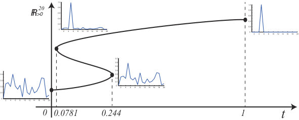 Figure 1
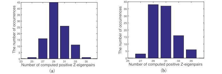 Figure 4
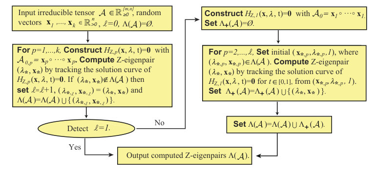 Figure 3