Harmonic Grammar, Optimality Theory, and Syntax Learnability: An Empirical Exploration of Czech Word Order
Ann Irvine, Mark Dredze
TL;DR
This paper empirically compares Harmonic Grammar and Optimality Theory learning algorithms, demonstrating that HG's greater expressivity leads to better Czech word order prediction, with the perceptron performing notably well.
Contribution
It provides a systematic comparison of HG and OT learning algorithms and shows HG's advantages in modeling Czech word order and variation.
Findings
HG outperforms OT in Czech word order prediction
Perceptron learns HG models approaching upper bound accuracy
HG models effectively capture observed variation
Abstract
This work presents a systematic theoretical and empirical comparison of the major algorithms that have been proposed for learning Harmonic and Optimality Theory grammars (HG and OT, respectively). By comparing learning algorithms, we are also able to compare the closely related OT and HG frameworks themselves. Experimental results show that the additional expressivity of the HG framework over OT affords performance gains in the task of predicting the surface word order of Czech sentences. We compare the perceptron with the classic Gradual Learning Algorithm (GLA), which learns OT grammars, as well as the popular Maximum Entropy model. In addition to showing that the perceptron is theoretically appealing, our work shows that the performance of the HG model it learns approaches that of the upper bound in prediction accuracy on a held out test set and that it is capable of accurately…
Click any figure to enlarge with its caption.
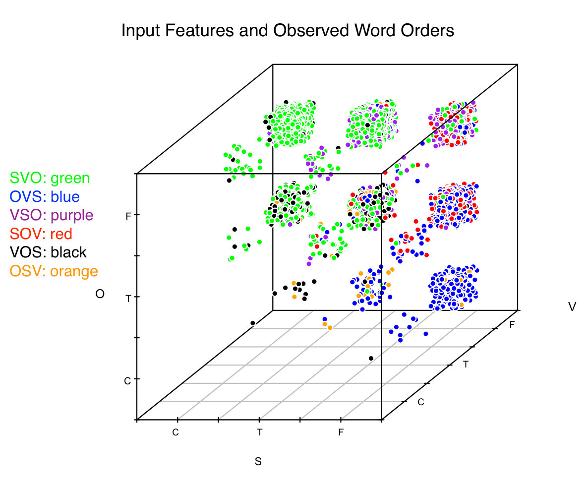 Figure 1
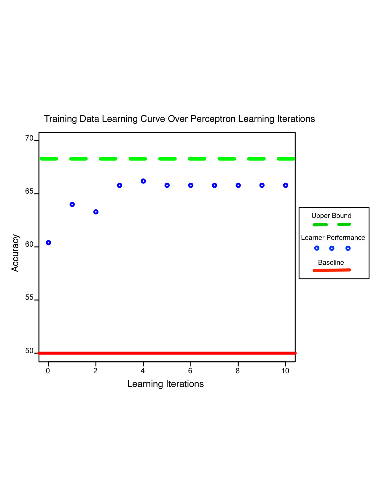 Figure 2
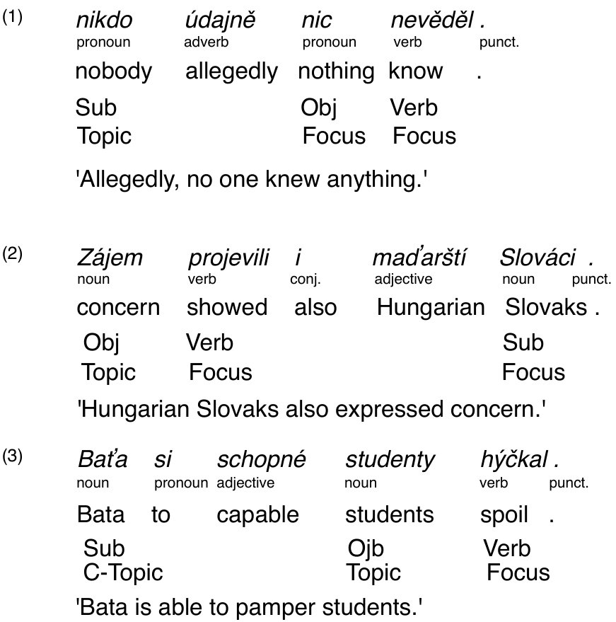 Figure 3
| Word | Percent of |
| Order | Corpus Sentences |
| SVO | 50.0% |
| OVS | 18.3% |
| VSO | 10.9% |
| SOV | 10.1% |
| VOS | 8.3% |
| OSV | 2.5% |
| Disc Func | Counts of Sentences with Basic Word Orders | % with Most | ||||||||
| S | V | O | SVO | OVS | VSO | SOV | VOS | OSV | Sum | Likely Order |
| T | T | T | 23 | 4 | 4 | 3 | 3 | 3 | 40 | 58% |
| T | T | C | 0 | 1 | 0 | 0 | 0 | 2 | 3 | 67% |
| T | T | F | 22 | 0 | 11 | 0 | 1 | 0 | 34 | 65% |
| T | C | T | 0 | 0 | 0 | 0 | 0 | 0 | 0 | - |
| T | C | C | 0 | 0 | 0 | 0 | 0 | 0 | 0 | - |
| T | C | F | 0 | 0 | 0 | 0 | 0 | 0 | 0 | - |
| T | F | T | 97 | 26 | 28 | 12 | 80 | 32 | 275 | 35% |
| T | F | C | 2 | 43 | 0 | 0 | 1 | 20 | 66 | 65% |
| T | F | F | 519 | 7 | 145 | 17 | 28 | 4 | 720 | 72% |
| C | T | T | 7 | 0 | 0 | 0 | 3 | 0 | 10 | 70% |
| C | T | C | 0 | 0 | 0 | 0 | 1 | 0 | 1 | 100% |
| C | T | F | 26 | 0 | 1 | 0 | 3 | 0 | 30 | 87% |
| C | C | T | 0 | 0 | 0 | 0 | 0 | 0 | 0 | - |
| C | C | C | 0 | 0 | 0 | 0 | 0 | 0 | 0 | - |
| C | C | F | 0 | 0 | 0 | 0 | 0 | 0 | 0 | - |
| C | F | T | 111 | 0 | 2 | 0 | 76 | 4 | 193 | 58% |
| C | F | C | 0 | 0 | 0 | 0 | 9 | 2 | 11 | 82% |
| C | F | F | 610 | 0 | 3 | 0 | 34 | 2 | 649 | 94% |
| F | T | T | 1 | 17 | 1 | 14 | 0 | 0 | 33 | 52% |
| F | T | C | 0 | 9 | 0 | 0 | 0 | 0 | 9 | 100% |
| F | T | F | 4 | 3 | 5 | 2 | 0 | 0 | 14 | 36% |
| F | C | T | 0 | 0 | 0 | 0 | 0 | 0 | 0 | - |
| F | C | C | 0 | 0 | 0 | 0 | 1 | 0 | 1 | 100% |
| F | C | F | 0 | 0 | 0 | 0 | 0 | 0 | 0 | - |
| F | F | T | 7 | 222 | 16 | 153 | 4 | 2 | 404 | 55% |
| F | F | C | 0 | 184 | 0 | 1 | 0 | 4 | 189 | 97% |
| F | F | F | 48 | 24 | 105 | 95 | 1 | 0 | 273 | 38% |
| Totals | 1477 | 540 | 321 | 297 | 245 | 75 | 2955 | 2013 | ||
| 50.0% | 18.3% | 10.9% | 10.1% | 8.3% | 2.5% | 68.1% | ||||
| Learner | OT/HG-Specific | Online | Prob Dist Output |
|---|---|---|---|
| Constraint Demotion | Yes | Yes | No |
| Gradual Learning Alg. | Yes | Yes | No |
| Perceptron | No | Yes | No |
| Maximum Entropy | No | No | Yes |
| Accuracy | |
|---|---|
| Baseline | 50.3% |
| Perceptron Performance | 67.0% |
| Upper Bound | 69.4% |
| Constraint | Learned Weight | Learned Ranking | ||||
|---|---|---|---|---|---|---|
| Run 1 | Run 2 | Run 3 | Run 1 | Run 2 | Run 3 | |
| C-Topic Left | 15.60 | 12.28 | 12.95 | 1 | 2 | 1 |
| Topic Left | 11.26 | 8.79 | 10.33 | 2 | 5 | 3 |
| Focus Right | 10.39 | 10.12 | 9.57 | 3 | 4 | 4 |
| Topic Right | 9.36 | 8.40 | 8.42 | 4 | 6 | 7 |
| Object Right | 8.63 | 13.29 | 10.41 | 5 | 1 | 2 |
| Focus Left | 8.36 | 7.79 | 7.98 | 6 | 8 | 8 |
| C-Topic Right | 7.21 | 7.34 | 8.69 | 7 | 9 | 6 |
| Subject Right | 7.18 | 12.01 | 9.01 | 8 | 3 | 5 |
| Object Left | 6.99 | 4.30 | 5.49 | 9 | 10 | 11 |
| Subject Left | 5.96 | 4.21 | 5.64 | 10 | 11 | 10 |
| Verb Left | 5.68 | 3.52 | 4.88 | 11 | 12 | 12 |
| Verb Right | 3.40 | 7.95 | 6.62 | 12 | 7 | 9 |
| Accuracy | 67.0% | 67.0% | 67.0% | |||
| Element | Difference Between Left and Right Aligned Constraint Weights, | |||
| Run 1 | Run 2 | Run 3 | Average | |
| C-Topic | 8.39 | 4.94 | 4.26 | 5.86 |
| Object | -1.64 | -8.99 | -4.92 | -5.18 |
| Subject | -1.22 | -7.80 | -3.37 | -4.13 |
| Focus | -2.03 | -2.33 | -1.59 | -1.98 |
| Topic | 1.90 | 0.39 | 1.91 | 1.40 |
| Verb | 2.28 | -4.43 | -1.74 | -1.30 |
| Training Prediction | Testing Prediction | Accuracy |
| Baseline | 50.3% | |
| Upper Bound | 69.4% | |
| ML prediction | ML prediction | 59.7% |
| ML prediction | SOT prediction | 47.4% |
| SOT prediction | ML prediction | 59.7% |
| SOT prediction | SOT prediction | 16.9% |
| Perceptron | 67.0% | |
| Constraint | Ranking Value | Ranking Value |
|---|---|---|
| Weights normalized | Spreading Value Normalized | |
| C-Topic Left | 8.82 | 51.88 |
| Focus Right | 8.63 | 50.76 |
| Object Right | 8.55 | 50.29 |
| C-Topic Right | 8.53 | 50.18 |
| Subject Right | 8.49 | 49.94 |
| Topic Left | 8.42 | 49.53 |
| Subject Left | 8.40 | 49.41 |
| Verb Left | 8.35 | 49.12 |
| Object Left | 8.26 | 48.59 |
| Verb Right | 7.96 | 46.82 |
| Topic Right | 7.85 | 46.18 |
| Focus Left | 7.76 | 45.65 |
| Focus Right | Obj. Right | Subj. Right | Topic Left | Subj. Left | ||
| SVO | x | x | ||||
| OVS | x | x | x | |||
| VSO | x | x | x | x | ||
| SOV | x | x | ||||
| VOS | x | x | x | x | ||
| OSV | x | x | x |
| Constraint | Weight | SOV | SVO | SOV | SVO |
| C-Topic Left | 15.60 | 0 | 0 | ||
| Topic Left | 11.26 | + | + | ||
| Focus Right | 10.39 | + | – | + 10.39 | – 10.39 |
| Topic Right | 9.36 | – | + | – 9.36 | + 9.36 |
| Object Right | 8.63 | – | + | – 8.63 | + 8.63 |
| Focus Left | 8.36 | – | – | ||
| C-Topic Right | 7.21 | 0 | 0 | ||
| Subject Right | 7.18 | – | – | ||
| Object Left | 6.99 | – | – | ||
| Subject Left | 5.96 | + | + | ||
| Verb Left | 5.68 | – | – | ||
| Verb Right | 3.40 | + | – | + 3.40 | – 3.40 |
| Sum of Differing Elements | – 4.2 | + 4.2 | |||
| Accuracy | |
|---|---|
| Baseline | 50.3% |
| GLA - ML Prediction | 59.7% |
| MaxEnt | 66.5% |
| Perceptron | 67.0% |
| Upper Bound | 69.4% |
| Constraint | Ranking Value |
|---|---|
| C-Topic Left | 2.30 |
| Subject Left | 0.53 |
| C-Topic Right | 0.39 |
| Object Right | 0.30 |
| Subject Right | 0.27 |
| Focus Right | 0.26 |
| Topic Left | 0.24 |
| Focus Left | 0.14 |
| Object Left | -0.04 |
| Verb Left | -0.18 |
| Topic Right | -1.00 |
| Verb Right | -1.33 |
| Algorithm | Weighted |
|---|---|
| GLA | 0.92 |
| Perceptron | 0.80 |
| MaxEnt | 0.53 |
| True | GLA | Perceptron | MaxEnt | |
|---|---|---|---|---|
| SVO | 16% | 44% | 39% | 43% |
| OVS | 5% | 11% | 26% | 19% |
| VSO | 31% | 25% | 19% | 16% |
| SOV | 47% | 0% | 2% | 4% |
| VOS | 1% | 20% | 14% | 16% |
| OSV | 1% | 0% | 1% | 2% |
| - | 5.56 | 2.00 | 1.59 |
| True | GLA | Perceptron | MaxEnt | |
|---|---|---|---|---|
| SVO | 67% | 65% | 64% | 62% |
| OVS | 0% | 5% | 16% | 4% |
| VSO | 25% | 17% | 11% | 21% |
| SOV | 3% | 0% | 2% | 6% |
| VOS | 5% | 10% | 6% | 3% |
| OSV | 0% | 3% | 1% | 3% |
| - | 0.36 | 0.34 | 0.14 |
| True | GLA | Perceptron | MaxEnt | |
|---|---|---|---|---|
| SVO | 0% | 11% | 8% | 10% |
| OVS | 96% | 82% | 79% | 74% |
| VSO | 0% | 5% | 3% | 4% |
| SOV | 0% | 1% | 1% | 1% |
| VOS | 1% | 1% | 4% | 3% |
| OSV | 3% | 1% | 5% | 8% |
| - | 0.26 | 0.23 | 0.30 |
| Predictor | Accuracy | |
|---|---|---|
| Uniform distribution over word order labels | 1.53 | 16.7% |
| Predict most likely single word order for input | 5.54 | 69.4% |
| GLA prediction | 0.92 | 59.7% |
| MaxEnt | 0.53 | 66.5% |
| Perceptron prediction | 0.80 | 67.0% |
| S-L | S-R | V-L | V-R | O-L | O-R | T-L | T-R | C-L | C-R | F-L | F-R |
|---|---|---|---|---|---|---|---|---|---|---|---|
| 9 | 3 | 2 | 4 | 8 | 1 | 5 | 6 | 4 | 1 | 3 | 8 |
| S-L | S-R | V-L | V-R | O-L | O-R | T-L | T-R | C-L | C-R | F-L | F-R | |
| 1 | -1 | -1 | -1 | -1 | 1 | 0 | 0 | 1 | -1 | -1 | 1 | |
| 9 | 3 | 2 | 4 | 8 | 1 | 5 | 6 | 4 | 1 | 3 | 8 |
| S-L | S-R | V-L | V-R | O-L | O-R | T-L | T-R | C-L | C-R | F-L | F-R | |
| -1 | 1 | -1 | -1 | 1 | -1 | 0 | 0 | -1 | 1 | 1 | -1 | |
| 9 | 3 | 2 | 4 | 8 | 1 | 5 | 6 | 4 | 1 | 3 | 8 |
| S-L | S-R | V-L | V-R | O-L | O-R | T-L | T-R | C-L | C-R | F-L | F-R | |
| -1 | -1 | 1 | -1 | -1 | 1 | 0 | 0 | -1 | -1 | 1 | 1 | |
| 9 | 3 | 2 | 4 | 8 | 1 | 5 | 6 | 4 | 1 | 3 | 8 |
| S-L | S-R | V-L | V-R | O-L | O-R | T-L | T-R | C-L | C-R | F-L | F-R | |
| 1 | -1 | -1 | 1 | -1 | -1 | 0 | 0 | 1 | -1 | -1 | 1 | |
| 9 | 3 | 2 | 4 | 8 | 1 | 5 | 6 | 4 | 1 | 3 | 8 |
| S-L | S-R | V-L | V-R | O-L | O-R | T-L | T-R | C-L | C-R | F-L | F-R | |
| -1 | 1 | 1 | -1 | -1 | -1 | 0 | 0 | -1 | 1 | 1 | -1 | |
| 9 | 3 | 2 | 4 | 8 | 1 | 5 | 6 | 4 | 1 | 3 | 8 |
| S-L | S-R | V-L | V-R | O-L | O-R | T-L | T-R | C-L | C-R | F-L | F-R | |
| -1 | -1 | -1 | 1 | 1 | -1 | 0 | 0 | -1 | -1 | 1 | 1 | |
| 9 | 3 | 2 | 4 | 8 | 1 | 5 | 6 | 4 | 1 | 3 | 8 |
| S-L | S-R | V-L | V-R | O-L | O-R | T-L | T-R | C-L | C-R | F-L | F-R | |
| SVO | 1 | -1 | -1 | -1 | -1 | 1 | 0 | 0 | 1 | -1 | -1 | 1 |
| SOV | 1 | -1 | -1 | 1 | -1 | -1 | 0 | 0 | 1 | -1 | -1 | 1 |
| SVO-SOV | 0 | 0 | 0 | - | 0 | + | 0 | 0 | 0 | 0 | 0 | 0 |
| 9 | 3 | 2 | 4 | 8 | 1 | 5 | 6 | 4 | 1 | 3 | 8 | |
| 9 | 3 | 2 | 3 | 8 | 2 | 5 | 6 | 4 | 1 | 3 | 8 |
Peer Reviews
No public reviews on file for this paper yet. If you reviewed it on a platform where reviews are public (OpenReview, ICLR, NeurIPS, ICML), you can paste yours below so the community can read it here.
Videos
No videos yet. Explain this paper in a talk, walkthrough, or lecture? Add one.
Taxonomy
TopicsNatural Language Processing Techniques · Speech Recognition and Synthesis · Speech and dialogue systems
∎
11institutetext: Ann Irvine and Mark Dredze 22institutetext: Department of Computer Science, Johns Hopkins University
3400 N. Charles St.
Baltimore, MD 21218
Tel.: 1-540-460-3663
22email: [email protected], [email protected]
Harmonic Grammar, Optimality Theory, and Syntax Learnability:
Ann Irvine
Mark Dredze
Abstract
This work presents a systematic theoretical and empirical comparison of the major algorithms that have been proposed for learning Harmonic and Optimality Theory grammars (HG and OT, respectively). By comparing learning algorithms, we are also able to compare the closely related OT and HG frameworks themselves. Experimental results show that the additional expressivity of the HG framework over OT affords performance gains in the task of predicting the surface word order of Czech sentences. We compare the perceptron with the classic Gradual Learning Algorithm (GLA), which learns OT grammars, as well as the popular Maximum Entropy model. In addition to showing that the perceptron is theoretically appealing, our work shows that the performance of the HG model it learns approaches that of the upper bound in prediction accuracy on a held out test set and that it is capable of accurately modeling observed variation.
Keywords: Optimality Theory, Harmonic Grammar, Learnability, Czech
1 Introduction
A complete theory of grammar must explain not only the structure of linguistic representations and the principles that govern them but also how those grammars are learned. Most of the work in Optimality Theory (OT) (Prince and Smolensky, 1993, 2004) has focused on discovering the constraint rankings that speakers use to produce and understand a given language, and how such rankings vary across languages. However, there have been several threads of research on modeling how speakers learn the constraint rankings in the first place. The earliest of the learnability research focused on OT grammars (Tesar and Smolensky, 1993; Tesar, 1995; Tesar and Smolensky, 1998, 2000; Boersma, 1997; Boersma and Hayes, 2001). However, recently there has been a resurgence of interest in the Harmonic Grammar (HG) framework (Legendre et al, 1990a, b, c, 2006a, 2006b; Coetzee and Pater, 2008; Pater, 2009; Jesney and Tessier, 2009; Potts et al, 2010), which is closely related to OT. In this work, we theoretically and empirically compare learning algorithms for each and, by doing so, are able to compare the frameworks themselves.
As noted in recent work, including Pater (2008), Boersma and Pater (2008), and Magri (2010), the perceptron learning algorithm is well-established in the Machine Learning field and is a natural choice for modeling human grammar acquisition. The algorithm learns from one observation at a time, and it is capable of learning from a noisy corpus of observed natural language. In this work, we make a case for the perceptron, which we use to learn a model that specifies a set of constraint weights relevant to one syntax phenomenon, Czech word order. We extract training data (sentences annotated with grammatical and information structure and their surface word orders) from the Prague Dependency Treebank (Hajic et al, 2001) and use basic alignment (edge-most) constraints on grammatical and information structure to predict the surface order of the subject, verb, and object. The perceptron algorithm learns how to numerically weight a set of constraints – a Harmonic Grammar.
Ordering HG constraints by the magnitude of their weights may specify a hierarchical constraint ranking, an OT Grammar, and doing so is the essence of the classic Gradual Learning Algorithm (GLA) (Boersma, 1997). Recent work (Magri, 2011) has pointed out that any HG learning algorithm can be adapted to learn an OT grammar and, thus, OT learnability is no more computationally complex than HG learnability. However, HG is a more expressive grammar framework. That is, all OT grammars can be expressed as HG grammars but not vice-versa. In this work, we automatically learn both types of grammars and show that the additional expressiveness of Harmonic Grammars results in gains in surface form prediction accuracies. That is, we use a held out set of empirical data to quantitatively evaluate each and find that allowing for so-called ganging-up-effects, the more expressive Harmonic Grammar models Czech Word Order more accurately than the OT grammar learned by the GLA. Furthermore, the performance of the HG grammar learned by the perceptron approaches that of the upper bound, which is defined in terms of the information available to any learner.
We compare the perceptron and GLA and the prediction accuracies of the grammars they learn with a Maximum Entropy model, another popular model of HG/OT learnability (Jaeger and Rosenbach, 2003; Goldwater and Johnson, 2003; Hayes and Wilson, 2008). Crucially, we show that, relative to the other two algorithms and our baseline strategies, the perceptron-learned grammars capture variation in production well.
All previous research on OT/HG learnability has focused on the phonological component of a grammar. To date there have been no thorough studies that explore the learnability of the syntax component of an OT grammar. In this work we contribute to the ongoing research comparing HG and OT and learning algorithms for each from the perspective of learning the syntax grammar component. In particular, our work:
- •
Explores the learnability of OT/HG syntax.
- •
Relies on observed data to empirically learn, evaluate, and directly compare grammars and learning algorithms.
- •
Uses the online perceptron algorithm to learn a Harmonic Grammar (HG).
- •
Demonstrates that ganging-up-effects provide HG an empirical advantage over OT in terms of modeling syntax.
- •
Directly compares the perceptron, the GLA, and a Maximum Entropy (MaxEnt) learner in terms of:
- –
Their theoretical applicability to the learnability problem,
- –
How accurately each learned model predicts the word order corresponding to a particular input,
- –
How accurately each models word order variation observed over a large corpus.
Our work shows that the perceptron is both theoretically and empirically attractive for modeling learnability and that Harmonic Grammars provide necessary additional power over OT grammars. Furthermore, we show that it is possible to empirically explore the learnability of the syntax component of HG/OT grammars.
2 Background
2.1 Optimality Theory and Harmonic Grammars
We assume that our readers are familiar with the Optimality Theory (OT) framework proposed in Prince and Smolensky (1993) and Harmonic Grammar (HG) proposed in Legendre et al (1990a), and we only briefly review each here. In OT, candidate surface forms are evaluated based on a hierarchical constraint ranking. Constraints are indicators on some element of a hypothesis surface form and, in some cases, also the input. In comparing a pair of candidates, the optimal candidate makes fewer violations of the highest-ranked constraints which distinguish the two. Importantly, constraints are violable. That is, the optimal surface form may violate some constraints. In iterating down through the hierarchy, once a candidate makes a violation that at least one other remaining candidate does not, it is immediately eliminated. If all remaining candidates violate a constraint, the process continues. The optimal surface form is the most harmonic.
In OT, harmony is defined by a total ordering over all candidate surface forms. In contrast, in HG, harmony is defined by a score associated with each candidate. In HG, a candidate’s harmony is determined by the sum of weights associated with each constraint that it violates. Low ranked constraints contribute to the harmony of candidates and, thus, may impact the choice of optimal surface form, including in cases where using strictly dominated constraints would have rendered them inconsequential. In other words, lower ranked constraints have the potential to gang-up on higher ranked constraints. A harmonic grammar which uses numeric weights can always express a hierarchical OT grammar. Weights would just need to be different enough that lower weighted constraints could never overpower higher ranked constraints, even cumulatively. The power of two series is one example of a series of weights that have this property: 1, 2, 4, 8, 16, 32, 64, 128, etc.
Although OT was proposed after HG, recently HG has regained research momentum in the community, e.g. Pater et al (2007); Coetzee and Pater (2008); Boersma and Pater (2008); Pater (2009); Potts et al (2010). However, it remains to be seen empirically if it offers advantages over OT to justify its additional complexity. Jesney and Tessier (2009) provide some evidence that ganging-up effects can be empirically observed. We further this claim and give a detailed discussion in Section 6.4.
2.2 Learnability
As pointed out in Johnson (2009), there are two, potentially separate, grammar learning problems. The first challenge is to define the structure of the learned grammar itself. This learning problem is also referred to as learnability. The second challenge is to explain the particular algorithm or process involved in learning. Much of this work is done under the name language acquisition. To date, linguists have addressed both facets of learning, usually focusing on one or the other.
The research literature on the learnability of an OT model of speakers’ knowledge of grammar and their production patterns, including variation, is extensive and includes the influential papers by Jaeger and Rosenbach (2003) and Goldwater and Johnson (2003). In contrast to the plethora of work on learning phonological grammars given both underlying and surface word forms, Jarosz (2006) learns phonological production patterns from surface forms alone. There is also some work in modeling, more specifically, a learner’s production patterns from the perspective of stages of language acquisition (Wilson, 2006; Legendre et al, 2004). The majority of work in this line of research models grammar using Maximum Entropy models, which are naturally capable of producing expected probability distributions over possible surface forms.
Somewhat separate are the efforts to model the particular learning algorithm that allows humans to acquire the grammar of a language. Since humans learn incrementally, from individual words and sentences in sequence, this line of research has focused on computational learning models that also learn from a sequence of individual words and sentences. The machine learning community refers to these algorithms that only look at one training example at a time as online. Algorithms that consider all of the training data available to them at once are, in contrast, called batch algorithms.
Tesar and Smolensky (1998, 2000) present the first set of algorithmic discussions. They propose an algorithm called Constraint Demotion (CD) and provide manual simulations of the process of learning a variety of phonological constraint rankings. Eisner (2000) discusses the computational complexity of the CD algorithm and extensions of it. Boersma (1997) and Boersma and Hayes (2001) present the Gradual Learning Algorithm (GLA), which learns an Optimality Theory grammar and is an alternative to the CD algorithm. In contrast to CD, the GLA may learn a Stochastic Optimality Theory (SOT) grammar, which can account for noisy input data and was proposed as way to learn production variation. Pater (2008) points out a flaw in the GLA algorithm and gives a high level discussion of the perceptron learning algorithm as a possible alternative. Boersma and Pater (2008) extend this idea and propose a Harmonic Grammar version of the GLA algorithm (HG-GLA), which is similar to the perceptron algorithm. The HG-GLA work provides a detailed theoretical exploration of the learning algorithm, including some learning computer simulations. Coetzee and Pater (2008, to appear) use the HG-GLA learner to model phonological variation. We explore each of these algorithms in more detail in Section 5.2.
3 Motivation
This work brings together the two threads of work on grammar learning described above. It follows the major intuition of the work done on the second, algorithmic challenge: the algorithms that model human learning should learn online, from one sentence at a time. It follows directly from recent theoretical discussions of such algorithms (Pater, 2008; Magri, 2010; Boersma and Pater, 2008) as well as a plethora of work on the properties of the perceptron algorithm (Rosenblatt, 1958). Additionally, like much of the previous work, it empirically evaluates the models learned by the algorithms, which should accurately predict observed surface forms, including patterns of variation over possible surface forms. Sections 5 and 6, below, give systematic theoretical and empirical comparisons of standard algorithms explored in the OT and HG literature including Constraint Demotion (CD), the Gradual Learning Algorithm (GLA), the perceptron, and the Maximum Entropy (MaxEnt) model. Throughout this work, we focus on learning from an observed, noisy corpus, and model a challenging grammatical phenomenon, Czech word order. Our major claim is that the perceptron is a good learner for the following reasons:
- •
It is an online (learns from one sentence at a time) learner.
- •
It is a simple learning algorithm, so it does not require complex models of broader cognition.
- •
It is well-studied and its properties are well-understood.
- •
It is accurate because it can allow for ganging-up effects.
- •
The model it learns does a good job of predicting observed variation.
Along the way, we show empirically that the additional complexity of Harmonic Grammars over Optimality Theory grammars yield higher prediction accuracies.
4 Czech Word Order
4.1 Phenomenon
Czech is a language with a relatively free word order (Naughton, 2012). That is, it is common to see all orders of subject, verb, and object in grammatical sentences. However, the basic order is SVO, and the surface word order is strongly influenced by the information structure, or discourse, notions of topic and focus. Topic is old information with respect to the current discourse, and it is usually aligned left in the surface order. Focus, on the other hand, is new information and is usually aligned right in the surface order (Hajičová et al, 1995). In this work, we automatically learn the ranking of constraints that dictate the Czech word order phenomenon.
The relationship between syntax, phonology, and discourse is complex and the subject of much prior work in linguistics, including Lambrecht (1994) and Kiss (1995). Using Russian as an example language, King (1995) discusses the interaction between these levels of structural encoding and, in particular, the implications for the scope of information structure elements. Like Russian, surfacing Czech word orders demonstrate the interaction between information structure and syntax structure.
In this work, we assume that information structure elements play a role in determining the surface word order of Czech sentences. We take one set of annotations, described below, as given, and do not explore the degree to which they are complete and correct. It is important to keep in mind, however, that the learning frameworks that we describe could incorporate any additional or different sets of similar annotations.
4.2 Data
Our dataset comes from the Prague Dependency Treebank (PDT) (Hajic et al, 2001). The PDT provides a very rich set of annotations, both automatically and manually created. It annotates dependency structure as well as part of speech, morphology, semantic relations, information structure, and more.
We selected a subset of the sentences in the PDT from which to learn and evaluate a grammar of Czech Word Order. We limited the set to those sentences that are declarative; have only a single, transitive predicate; and which do not contain commas (which often indicate dependent clauses, relative clauses, or information structure functions). Additionally, we trim prepositional phrases from these sentences, which allows us to focus on the subject, verb, and object elements, and their order. The sentences are simple and, thus, simple to learn from. Table 1 shows the frequency of different word order patterns found in a set of 2955 simple, fully annotated, transitive sentences in the PDT.
Each word in each sentence in the PDT is annotated with one of the following (Hajičová et al, 1998; Buráňová et al, 2000):
- •
t=non-contrastively contextually bound [topic, or old information]
- •
c=contrastive contextually bound expression [contrastive topic, or contrastive old information]
- •
f=contextually non-bound expression [focus, or new information]
f, or focus, is the default annotation. Along with grammatical function (S, O, V), these annotations on unordered words form the input to the grammar. Three example sentences are given in Figure 2.
4.3 Constraint Set
Choi (1999) gives a full discussion of word order variation from an Optimality Theory perspective. That work explores German and Korean and suggests OT constraints that place elements with certain salient information structure properties (e.g. newness, prominence) in particular positions in the sentence (e.g. preverbal, sentence initial). We refer readers to Choi’s detailed review of the interaction between constituents and their information and discourse structure properties. The algorithms that we discuss in this work could learn rankings of any proposed, violable OT constraints.
We use a very simple set of 12 alignment constraints, which are also sometimes called edge-most constraints (Prince and Smolensky, 1993, 2004; McCarthy, 2003). In this work, the alignment constraints are a binary, not distance-based, indication of whether or not an element is aligned to the edge of a sentence. Our constraints are similar to those used by Costa (1997, 2001), who used an OT framework to explain variation in unmarked word orders over many languages. Unlike that work, we use alignment constraints on grammatical structures in addition to information structure markers. Six of our constraints are grammatical structure alignment constraints corresponding to the left and right alignment of the subject, verb, and object (e.g. subject left). Similarly, six are information structure alignment constraints corresponding to the left and right alignment of each of the information structure markers enumerated in Section 4.2. All alignment constraints are evaluated with respect to entire sentences, not, for example, with respect to the verb phrase only. Specifically, these universal alignment constraints are:
- •
Grammatical structure alignment constraints:
- –
Align Subject Left
- –
Align Subject Right
- –
Align Verb Left
- –
Align Verb Right
- –
Align Object Left
- –
Align Object Right
- •
Information structure alignment constraints:
- –
Align C-Topic Left
- –
Align C-Topic Right
- –
Align Topic Left
- –
Align Topic Right
- –
Align Focus Left
- –
Align Focus Right
Formally, the Align C-Topic Left constraint is given by:
Align C-Topic Left: Contrastive topics are sentence initial. Failed when a contrastive topic exists in the sentence and a contrastive topic is not sentence initial. Vacuously satisfied if a contrastive topic is not present in the sentence.
The formal definitions of the other alignment-based constraints follow directly from this.
Each of the 12 constraints is violated when the surface word order does not obey the stated left or right alignment. For example, an SVO surface word order violates the constraints align subject right, align verb left, align verb right, and align object left. Also for an SVO surface word order, if the subject is marked as a contrastive topic and the verb and object are both marked as focused elements, then the constraints align c-topic right and align focus left are violated. The constraints align topic left and align topic right are vacuously satisfied as there is no topicalized element in the example sentence.
4.4 Data Variation
The sentences and corresponding annotations that we extract from the PDT include variation due to optionality and also variation due to incomplete information, or sentence representations. The machine learning community refers to this type of variation, legitimate or not, as noise in the data. The learning algorithms that we use to automatically make sense of the data must be tolerant of these types of variation, or noise.
First, the data includes evidence of true variation, or grammatical word order optionality. That is, for some meaningful content situated in a particular discourse context, there may be more than one grammatical word order (e.g. speakers may have the option of using SVO or SOV order). Second, some of the observed variation in the data may be due to grammar or information structure that we do not consider. That is, if we considered additional properties of a given sentence, it may be possible to explain away why one word order is observed instead of another. Teasing apart true variation and variation due to incomplete information would require having native Czech speakers closely examine each sentence in our dataset as well as their discourse context (preceding sentences) and give detailed additional annotations, possibly beyond those represented in the PDT. In this section, we present the data and a discussion of the variation that we observe in it. Furthermore, we describe lower and upper bounds on word order prediction accuracy, given the input to the learners, which determine what we expect and hope for our learning algorithms to achieve on similarly behaved data.
Table 2 shows input feature patterns (all combinations of subject, verb, and object marked by topic, contrastive topic, or focus) and the frequencies of observed surface word orders. This data provides an upper bound on how well we can expect learning algorithms to be able to predict word order, given only the information structure of the subject, verb, and object. There are 27 input patterns (each of S, V, and O marked with either T, C, or F). Given only this information, the best any learner can do is to produce the most likely word order for each input pattern, which would achieve 68.1% accuracy on the training data. In Section 6.1, we will say that the prediction strategy of memorizing the single best word order for each of the 27 input patterns is the upper limit in model performance for predicting the word order of a sentence. This strategy is the upper bound because no additional information about the sentence will be available to the learner.
Table 2 also shows that, given no information about the information structure of the elements in a sentence, the best strategy for predicting word order is to, simply, always predict SVO. This approach would correctly predict the word order of 50.0% of the sentences represented in the table. In Section 6.1, we will refer to this as the baseline strategy for predicting the word order of a sentence.
Figure 2 is a visualization of the data in Table 2. The 27 input patterns are shown in clusters on a three dimensional plot. The axes correspond to grammatical structure (S, V, and O) and values along each axis correspond to the information structure associated with each for a particular sentence in the training data. Colors indicate the word order of the observed sentences. It is easy to see that most clusters are dominated by one or two word orders and that some input patterns (like V-C) rarely, if ever, occur in the data. Finally, many of the clusters are dominated by either SVO or OVS word orders, but there is little overlap of the two within a single input pattern. SVO more often occurs with input patterns that also yield VOS while OVS more often occurs with input patterns that also yield VSO and SOV.
It is important to recall here that the input information shown in Table 2 and Figure 2 (e.g. the verb is focused, or the subject is topicalized) is not directly used in learning. Rather, this information, in combination with a hypothesis (a word order), determine which constraints are violated. The input to the grammar consists of the constraint violations for a given candidate word order. In Section 5, we show how weights corresponding to constraints are learned and then used to predict labels on new data.
In addition to predicting the single most likely word order for a given pattern of input, we would like the grammars that our algorithms learn to be able to predict the observed variation in word order outputs (Bresnan, 2007; Doyle and Levy, 2008). That is, for example, we would like learned grammars to output SVO as the most likely word order for a topicalized subject and a focused verb and object and, additionally, output some probability distribution over the output word orders that indicates that VSO also has a fairly high probability, though it is not as high as that of SVO (see Table 2).
5 Learning
5.1 Perceptron Algorithm
The perceptron algorithm was introduced by Rosenblatt (1958) as a theory of the way a hypothetical biological nervous system stores and learns information. Since then, the algorithm has become a popular method in machine learning for doing supervised, discriminative classification (Littlestone, 1988) and there is considerable research expanding Rosenblatt’s original proposal (e.g., Collins (2002); Khardon et al (2005)).
Supervised learning algorithms like the perceptron learn to make predictions, such as a label in the case of discriminative classification, about input data given training examples that contain both input data and the true value of some underlying form, such as a label. In this work, we train a perceptron discriminative classifier, which chooses among the six possible sentential word orders (SVO, SOV, etc.). Training data takes the form of constraint violations determined by information structure markers on grammatical elements (e.g. subject is topicalized), the input data, and the corresponding observed word order pattern (the label). Using a supervised learning algorithm like the perceptron is a natural way to model human language learning since human learners also learn from observing labeled examples (individual sentences are supervised examples, and humans observe their word order).
The perceptron is an online algorithm, i.e. it updates its parameters based on one example (in this case, one sentence) at a time. Its only learned parameter is a single list of weights, each of which is associated with one attribute333The machine learning community refers to these as features. For clarity in this linguistic context, we refer to them as attributes.. Attributes indicate the value of some property of a single input example. In this work, attributes correspond to HG/OT constraints and the perceptron learns weights associated with each. A hypothesis (word order) is scored by computing a linear combination of attribute values (given the input and hypothesized label) and the corresponding weights.444For example, say the model only contains two attributes, A and B, and the current model weight vector gives A a weight of 3 and B a weight of 5, or . If some input and hypothesis has attribute values of and , and , then the resulting score would be , or . Following Boersma and Pater (2008), in this work, all attribute values are one of the following: , indicating that the input and hypothesis explicitly complies with a constraint; [math], indicating that a constraint is vacuously satisfied; or , indicating the input and hypothesis violate a constraint. That is, the harmony, or linear combination of weights, of a hypothesis is a function of the constraints that it complies with as well as those that it violates. Boersma and Pater (2008) point out that this setup is not explicitly disallowed by the original formulation of OT, which did not distinguish between overt constraint satisfaction and vacuous constraint satisfaction.
The perceptron’s learning is mistake-driven. That is, it only updates its parameters when it makes a mistake in predicting the label of an item in the training set. It iterates through the training data one example at a time, predicts the label of each example given its current parameters, and, finally, if its prediction doesn’t match the true label, it updates its weight vector accordingly.
Specifically, the prediction function is:
[TABLE]
where is the predicted label, for input , which has the highest score among all possible labels . Scores, or, in our case, harmonies, are calculated by multiplying the attribute vector, , by a vector of the current weights, . The indicates the dot product between the two vectors. As mentioned, in this work, each attribute has a value of (the constraint associated with the attribute is complied with, given the input and the hypothesis ), [math] (the constraint is vacuously satisfied), or (the constraint associated with the attribute is violated).555This setup could easily be translated into one where all attributes have a value of or [math] by doubling the attribute set to include one attribute for complying with each constraint and one attribute for violating each constraint. Appendix A explains the / attributes in detail. The update function for learning is as follows:
for each training example :
where is the true label, is the predicted label, is the current weight vector, is the updated weight vector, and is a learning rate parameter. The difference between the attribute values for the true label and for the predicted label () is the set of attributes (constraints) over which the true and predicted labels differ. If the true and the predicted labels are the same, the difference is zero and no update is made.
Appendix A gives a detailed example of how the perceptron algorithm learns a weight vector corresponding to the twelve constraints listed in Section 4.3 from the PDT data described by Table 2.
5.2 Comparison with Other OT Learners
In this section, we give intuitive, theoretical comparisons of the perceptron learner with algorithms used in previous OT/HG learnability research: the Constraint Demotion (CD) algorithm, the Gradual Learning Algorithm (GLA), and the Maximum Entropy (MaxEnt) classifier. Table 3 summarizes the discussion.
Constraint Demotion (CD) was the first OT learning algorithm to be proposed (Tesar and Smolensky, 1998, 2000). The CD algorithm assumes that there always exists a discrete, hierarchical constraint ranking, and the ranking is updated when the learner observes a piece of evidence for which she would not have produced the proper surface form, given the input data. Say the winner is the true, observed surface form and the loser is the surface form that the current model incorrectly predicted. The update function demotes all of the constraints that the winner violated which are currently ranked higher than the highest ranked loser’s constraint violation. At the end of the update, the learner is guaranteed to correctly predict the true, observed surface form. This algorithm, like the perceptron, is online and mistake-driven. However, it is not at all robust to data variation and will result in endless rank swapping if multiple surface forms for a single input are observed. Tesar and Smolensky (2000) discuss this limitation in detail, and it is the motivation for the Gradual Learning Algorithm, which was proposed soon after CD.
Boersma (1997) is the first presentation of the Gradual Learning Algorithm (GLA), which is an extension of the CD algorithm aimed at making it more robust to data variation. In the GLA, instead of aggressively demoting constraint rankings, numerical weights are associated with each and these are gradually updated666The size of the updates is a model parameter. In the perceptron formulation, this value is generally referred to as the learning rate. In the original GLA proposal, it is called the plasticity. when the learner makes mistakes. Thus, the GLA updates are similar to the perceptron algorithm’s updates. However, at the time of prediction, the GLA uses the magnitude of the weights to determine a discrete, non-numerical OT constraint ranking, and it uses the OT ranking to predict surface forms. Additionally, in order to account for data variation, the GLA may learn a Stochastic Optimality Theory (SOT) grammar rather than a traditional OT grammar. An SOT grammar adds some random noise777The noise is sampled from a zero mean, standard deviation one Gaussian and multiplied by a model parameter, called the spreading value in the original proposal of the GLA to the values of each constraint before extracting an OT constraint ranking and predicting the surface form. Like the perceptron and CD, the GLA is online and mistake-driven. However, it is different from the perceptron in that it uses an OT or SOT constraint ranking moel for predicting surface forms, not allowing for so-called ganging-up-effects.
Recently, Boersma and Pater (2008) proposed a Harmonic Grammar version of the GLA, HG-GLA. This algorithm learns just like the perceptron and the authors replicate perceptron proofs of convergence to explain some of the theoretical properties of the HG-GLA. Because that work is preliminary and only includes computer simulations, we do not adopt its terminology.
Maximum Entropy (MaxEnt) models, or log-linear models, are frequently used in the Machine Learning community for many classification tasks. Like the perceptron, MaxEnt models learn a vector of weights associated with each attribute function defined for the dataset (in our case, 12 constraints). However, MaxEnt learners seek to mimic training data distributions (while otherwise assuming as much variance, or uniformity, in the model as possible) and are designed to, by exponentiating and normalizing the linear combination of weights and attributes for a given input, produce a probability distribution over output labels, or surface word orders, in our case. Therefore, unlike the CD, perceptron, and GLA, the output of a MaxEnt classifier is a probability distribution over outputs. The most probable label, or surface form, is the maximum likelihood prediction for a given input. In contrast, the other three algorithms most naturally produce only a single maximum likelihood output prediction, and we must do some extra work888Such as inserting some random variation and sampling from outputs. to produce a distribution over output labels.
MaxEnt classifiers are typically learned in batch mode, not in an online setting like CD, the GLA, or the perceptron. That is, the model parameters are estimated by looking at all of the training data at once, not one sentence at a time. However, unlike CD and the GLA but like the perceptron, the MaxEnt model allows for violated low ranked constraints to collectively outrank a violation of a higher ranked constraint. Goldwater and Johnson (2003) use a MaxEnt model to learn probabilistic phonological grammars both with and without variation. That work uses a MaxEnt model to explain variation in Finnish genitive plural endings as accurately as the GLA model does and it claims that the model is more theoretically sound than the GLA. Jaeger and Rosenbach (2003) use a MaxEnt model to predict variation in the English genitive construction999e.g. the mother’s future vs. the future of the mother and provide some evidence that it is superior to the GLA model because of its ability to allow for ganging-up effects of low ranked constraints. Finally, Hayes and Wilson (2008) use a MaxEnt model to learn a model of phonotactic patterns and Pater et al (2010) explore the model’s convergence properties.
In this work, we claim that the perceptron has the benefit of being an online (one sentence at a time) learner, like CD and the GLA, but that it is able to outperform those algorithms because it uses the HG formalism and allows for ganging-up effects, like MaxEnt models. Although it does not naturally produce probability distributions over output labels, like MaxEnt models, we show in Section 7.1 that it does a good job of predicting variation. Additionally, it has the advantage of being a simple but well-established and well-studied learning algorithm.
5.3 Data Setup
For learning, the set of 4955 simple sentences extracted from the PDT are split into training, development, and test sets. The parameters (constraint weights) for a Harmonic Grammar are learned from the 2955 training data sentences. The 1000 development set sentences are used to choose a specific learning model (we explore several variants of the perceptron learning algorithm), and the remaining held-out 1000 test set sentences are used for evaluation after we identify a final model and parameters.
The subject, object, and predicate in each of the sentences is annotated as topicalized, contrastively topicalized, or focused. The attribute functions use these annotations and the hypothesis (a word order) to determine whether or not each constraint is violated (i.e. whether each of the 12 attributes has a value of , [math], or for some input and word order). As usual, a single weight vector is learned from the entire dataset. The constraint set and attribute functions are identical for learning GLA, perceptron, and MaxEnt models.
5.4 Perceptron Limitations and Modifications
The perceptron has several well-known limitations. These include slow convergence time and an inability to account for unbalanced data (in terms of attribute values and/or output labels). In order to overcome these limitations, we make some standard slight modifications to the algorithm and choose our final learning setup by measuring performance on the 1,000 sentence development set.
Learning iterations Because the perceptron converges slowly, we have it learn over many iterations over the training data. This is standard practice in the machine learning community, where the availability of supervised data is often an issue. It is also a reasonable strategy from the viewpoint of human learnability. Our data sample really contains sentence types, rather than sentence tokens. Our learner does not have access to the lexical items in a given instance in the training data (e.g. every sentence of type Subject-T, Verb-F, Object-T looks the same to the learner, no matter the actual words in the sentence). Therefore, as long as our sample of input types is representative and we can assume that a human learner would observe a constant distribution of input types over time (e.g. a child observes the same frequency of Subject-T, Verb-F, Object-T sentences in her first month as she does in the second month), then iterating over a single set of types is a reasonable approach. However, we do find that learning converges over just a few iterations over the training data, as shown in Figure 3.
Learning in the presence of noise Although the perceptron is fairly tolerant to noise (in our case, true variation in the data), it is not completely immune. In order to increase its resistance, we implement a slight modification to the original algorithm. The -trick, explained in Khardon et al (2005), allows the algorithm to ignore training examples that it repeatedly misclassifies, that is, those examples which look like they contain noise. In other words, it helps the algorithm learn to ignore sentences that look very different from the rest of the data. Predictions are made as follows:
[TABLE]
where is an indicator function that is 1 if is the correct label and 0 otherwise. is a counter that gives the total number of times example has been incorrectly classified and is a learning parameter. So, as increases, will eventually dominate the sum for the correct label , resulting in the correct prediction and no update. As before, is the predicted label, for input , which has the highest score among all possible labels . Scores, or, in our case, harmonies, are calculated by multiplying the attribute vector, by a vector of the current weights, . It is important to keep in mind that this ‘trick’ is only used in training, of course.
Again, this modification is reasonable from the perspective of human language acquisition; there may be factors that would enable a human learner to recognize which sentences are different from the rest (e.g. spoken emphasis) or, simply, a sentence may be different enough from the others that the listener assumes it is wrong.
Update normalization Finally, the perceptron is not good at learning when the training data is not well balanced with respect to attributes or output labels, and the PDT dataset has both types of unbalances. In order to account for this limitation, we normalize the update values using counts of the number of times a given attribute is either directly complied with or violated, but not vacuously satisfied, in the training data. For example, there are many sentences in the training data that have no contrastive-topical element. For those sentences, both align c-topic right and align c-topic left are vacuously satisfied. Therefore, the number of times that these attributes directly apply to a sentence is less than, for example, align subject left, which applies to all sentences because every sentence has a subject. When an update is made to an attribute, we divide by the normalization factor for the attribute. As a result, the size of the updates made to align c-topic right is greater than, for example, the size of the updates made to align subject left. This is a reasonable normalization technique since we want less frequent attributes to have the chance to achieve the same constraint weight magnitude as more frequent attributes.
6 Results
6.1 Perceptron Word Order Prediction Accuracy
In Section 4.4, we described the baseline prediction strategy (always predict SVO) as well as the upper bound (consider the complete input and predict the most probable label) for predicting the word order of a Czech sentence given the information available to our learning algorithm. Accuracy is defined as the percent of test set inputs for which a given model correctly predicts the surface word order. Table 4 shows these accuracies on a held out test set as well as the accuracy of the model learned by the perceptron algorithm. As the results show, the perceptron’s model drastically outperforms that baseline and its accuracy is within 2.5% of the upper bound.
6.2 Harmonic Grammar Weights
Three sets of constraint weights learned by three randomly initialized runs of the perceptron learning algorithm are shown in Table 5. It is interesting to see that the weights as well as the overall relative rankings do vary between the runs. However, the right/left preference for each information structure element (C-Topic, Topic, Focus) and two of the grammatical structure elements (Subject, Object) does not vary. Table 6 shows the difference between the learned weight for the left alignment constraint and the learned weight for the right alignment constraint for each element. All runs prefer C-Topic to be left, Topic to be left, and Focus to be right. Similarly, all runs prefer the object to be right and, perhaps contrary to expectations because the most common Czech word order is SVO, the subject to be right. The only element for which the learners do not learn a consistent alignment preference is the verb. However, all weights learned for the verb constraints are relatively small. In fact, this indicates that the model prefers the the verb to be neither left nor right but, rather, in the middle. That is, the when the verb is in the middle of a sentence, both of its alignment-based constraints are violated but neither penalty (constraint weight) is large. This is consistent with the fact that the two most frequent word orders are SVO and OVS.
Additionally, Tables 5 and 6 clearly show that the learned constraint weights have the same order of magnitude. That is, the weights of the lower ranked constraints are not so much less than those of the higher ranked constraints that we would never expect them to influence the word order output. In contrast, the relative magnitude of the lower ranked constraints indicate that so-called ganging-up-effects may be important and occur somewhat frequently. Below, in Section 6.3, we compare the perceptron with the GLA and empirically show that allowing for such effects leads to better word order prediction accuracies.
6.3 Empirical Comparison with the GLA
As explained in Section 2.1, a Harmonic Grammar (Legendre et al, 1990a) uses the particular numeric values of constraint weights to calculate scores, or harmonies, for input data and each possible word order, and the word order that scores the highest is chosen as the surface form. In contrast, the output from an Optimality Theory grammar is based only upon the relative, strict ranking of the set of constraints. As explained in Section 5.2, the Gradual Learning Algorithm learns numeric weights in a very similar way to the perceptron but the OT grammar that it learns makes word order predictions based upon a hierarchical OT ranking, which is inferred from the current weight vector. That is, the highest weighted constraint is the top ranked constraint, the second highest weighted is the second ranked constraint, and so on. In this Section, we empirically compare a model learned using the perceptron with a model learned using the GLA. The GLA and perceptron are very similar learning algorithms. Both make updates to weight vectors associated with constraints in the same way. However, they use different grammars (the GLA uses OT or SOT and the perceptron HG) to make predictions during training, which dictate which training examples are used to update the model. Because the learning algorithms are so similar, differences between prediction accuracies can be attributed to the difference between predicting word order using numeric (HG) constraint weights and using a hierarchical (OT) constraint ranking (see Section 6.4 for examples and further discussion).
We implemented the maximal GLA learning algorithm described by Boersma (1997). Like that implementation, we used a plasticity (learning rate) value of 0.01 and, using our development data, optimized the ranking spreading parameter, obtaining a value of 2.0.101010In our experiments, we found that the plasticity values between .001 and .5 did not affect performance much on the development data one way or the other and performance decreased with higher and lower values. Similarly, with plasticity at .01, we found that relative spreading values between 1.0 and 4.0 resulted in the best performance, with lower and higher values negatively impacting KL-divergence, see below. Plasticity is the magnitude of the weight added to or subtracted from constraint weights at each iteration of training. The relative spreading parameter is used in predicting surface forms. The product of the spreading parameter and some random noise111111Gaussian distribution with mean 0, standard deviation 1. is added to or subtracted from each constraint weight before the hierarchical OT relative rankings are inferred, which happens just before prediction. Like using the perceptron to learn a model, we iterated over the data several times before the GLA model converged.
In the formulation of Stochastic Optimality Theory given in Boersma (1997), noise is added to the current constraint ranking values (weights) before the learner predicts a surface form (in our case, a word order). Thus, in production, the learner chooses an expected word order from her current probability distribution over possible word orders rather than always predicting the most likely word order. Predicting the most likely word order, or using a maximum likelihood strategy, would minimize prediction errors, maximizing accuracy. In this section, we report results from using both the standard GLA strategy, henceforth SOT prediction, and the maximum likelihood strategy, henceforth ML prediction for both predicting test data surface forms and for predicting training data labels, which determines when updates to the ranking values are made. Table 7 shows the results.
Tables 4 and 7 show that even the best performing model learned by the GLA, which uses the ML strategy for prediction, does not perform nearly as well as the HG model learned by the perceptron. As mentioned above, this difference should be attributed to the difference between predicting word order using numeric (HG) constraint weights and using a hierarchical (OT or SOT) constraint ranking.
Table 8 shows the ranking values learned by the GLA when the SOT prediction strategy is used for predicting labels during training. For each grammatical and information structure element, the relative order of the left and right alignment constraints (e.g. Focus Right and Focus Left) is the same as the relative order between the two constraints in the first run of the learned perceptron weights in Table 5. In comparison with Table 5, the range of the GLA weight values is very small. However, the two are not easily comparable since the HG weights are cumulative and the GLA weights are used to infer a hierarchical ranking. It is interesting to note, however, the differences between the ranking values compared with the spreading value, which is normalized to 1.0 in the second columns of weights. That is, for example, it is likely that enough noise will be added to the Object Right, C-Topic Right, or Subject Right constraints such that their relative order will change. In contrast, it is unlikely the Focus Right and Focus Left constraint values would change enough for their relative orders to swap. It should also be noted that in ten runs, the relative ranking of the GLA-learned constraints did not vary at all. The ranking values shown in Table 8 are from one randomly chosen run.
6.4 Ganging-Up Effects
As mentioned in Section 6.3, the differences between the GLA-learned OT word order prediction accuracy and the perceptron-learned HG word order prediction accuracy can be attributed to the fact that the GLA uses a hierarchical set of constraints (an OT or SOT grammar) and the perceptron uses numeric constraints (an HG grammar). Since numeric weights can always express a hierarchical grammar, it is important to question whether or not the additional expressivity of an HG grammar allows us to account for actual, observed grammar phenomena.
Indeed, the model learned by the perceptron does outperform the GLA ML model in terms of accuracy, and in this section we closely examine some observed so-called ganging-up effects which cause this increase in performance. That is, we present a concrete example of when the inferred hierarchical prediction (GLA) doesn’t make the right prediction but allowing lower ranked constraints to gang-up on higher ranked constraints (perceptron) does result in the correct prediction.
One clear illustration of ganging-up effects is in predicting the input pattern of a topicalized subject and object and focused verb (line 7 of Table 2). Given the GLA rankings shown in Table 8 and the perceptron weights shown in Table 5, the GLA makes the maximum likelihood prediction (not inserting noise into the ranking values before prediction) of an SOV word order. In contrast, the perceptron weights predict SVO. In fact, as shown in Table 2, SVO is the most likely word order for this input pattern in the training data. The same is true for the test data, making SVO the better prediction. Note that the weights learned in all of our perceptron runs predict SVO for this input, and we will use the weights given in the first run of Table 5 for illustration.
First, we show the GLA ML prediction in the tableau in Table 9. For convenience, we leave out C-Topic Left, the highest ranked constraint, and C-Topic Right, the fourth highest constraint, because, since there is no contrastively topicalized element, all word orders vacuously satisfy those two constraints. The OT tableau shows that all word orders except SOV and OSV are eliminated by the high ranked Focus Right constraint and both SOV and OSV have the same violations on the Object Right, Subject Right, and Topic Left constraints. OSV violates the Subject Left constraint, leaving SOV as the predicted surface form. Note that we do not display the lower-ranked constraints, which are inconsequential to this analysis.
Next, we show the perceptron-learned model’s prediction for this input pattern. For simplicity, we only show the cumulative weights for SOV, predicted by the GLA-learned grammar, and SVO, which is the most harmonic word order under the perceptron-learned constraint weights. Table 10 shows how the perceptron-learned harmonic grammar scores each word order. The four constraints for which the possible word orders have differing violation patterns are highlighted in bold. Like the GLA OT predictor, the Focus Right constraint is the highest weighted constraint to discriminate between SOV and SVO. However, the table also shows that both Topic Right and Object Right have relatively high weights and also discriminate between the two surface word orders. Therefore, even though SVO violates Focus Right and SOV does not, its final score is higher than that of SOV because it does not violate Topic Right and Object Right, and those constraints gang-up on the higher weighted Focus Right.
This example of ganging-up effects shows how the expressivity of a Harmonic Grammar, which is beyond that of the hierarchical constraints in an Optimality Theory grammar, can result in a model which is capable of predicting correct surface forms that an OT model cannot predict. There are several additional input patterns in our small dataset and set of constraints that illustrate the same thing. These examples account for all of the over 7% surface form prediction accuracy discrepancy between the perceptron learner and the GLA learner.
6.5 Empirical Comparison with a MaxEnt Model
We know in advance that the Constraint Demotion (CD) algorithm is incapable of learning a grammar from data that includes variation like ours, and we have shown empirically that the perceptron learner outperforms the GLA since the models it uses allow for ganging-up effects. In this section, we briefly compare the perceptron with a Maximum Entropy (MaxEnt) model, which also uses numerical weights and allows for the same effects.
Table 11 shows the prediction accuracies of the GLA (maximum likelihood predictions) OT grammar and perceptron HG grammar, both reported above, in addition to the accuracy of a MaxEnt model. We used the Natural Language Toolkit (Bird et al, 2009) implementation of a MaxEnt model and a conjugate gradient based algorithm to learn the grammar. The relatively small difference between the perceptron and MaxEnt accuracies is statistically significant.121212Using a one sample Student t-test to compare the MaxEnt model’s accuracy with the distribution of perceptron accuracies, estimated by sampling the performance of twenty perceptron-learned models. The difference is significant to the .0001 level.
Table 12 shows the weights associated with each attribute that are learned by the MaxEnt learner. Although it is somewhat difficult to interpret these weights, which are exponentiated in the model, we can compare their relative ranking with that of the weights learned by the perceptron. In comparison with the first run reported in Table 5, the relative order of the left and right alignment constraints is the same for every grammatical and information structure element except for the subject.
7 Predicting Variation
The attribute weights that the perceptron algorithm learns are intended to predict the single best word order in the set of possible orders. However, in this section we would like to predict a distribution over word orders and compare that distribution with the one observed for each input pattern (see Table 2).131313For example, we would like the learner to predict both VSO and SOV with high probability and SVO with lower probability when the S, V, and O are all focused elements, the last line in Table 2.
In order to use the perceptron’s learned weights to predict such probability distributions, we use Noisy HG, which was proposed by Boersma and Pater (2008). That is, for each constraint, we take a noise sample from a zero-mean Gaussian141414Similar to our tuning for the GLA algorithm, we used our development set to tune a single parameter, the Gaussian variance, to .001 and add it to the current weight value. For each input pattern, we repeatedly sample and predict, keeping up with how many times each label is predicted. The sample predictions define a probability distribution over output labels. For both the GLA and the perceptron, we take 1,000 samples of the predicted word order for each input pattern.
Inserting noise into the perceptron-learned weights and the GLA-learned ranking values allows us to directly compare how well each predicts variation in our observed, held-out test data. As explained in Section 5.2, the MaxEnt model naturally produces distributions over outputs, or surface word orders.
7.1 Results
KL-divergence is a measure of the difference between probability distributions (Kullback and Leibler, 1951). In order to compare the GLA-learned SOT grammar, perceptron-learned HG grammar, and the conjugate gradient learned MaxEnt grammar in terms of predicting data variation, we compute the KL-divergence between the true, empirically observed distribution over output labels in our test set and the distribution predicted by a given grammar. We compute this distance metric for each of the 27 input patterns for which there is some observed data. We then take a weighted average over the 27 inputs and output distributions based on the number of observed sentences in the test data. Table 13 presents these aggregate results. The GLA and perceptron algorithms are trained on 50 iterations over the training data and with the model parameters optimized as described above. The KL-divergence is averaged over ten runs. Smaller KL-divergence values indicate better estimates of the probability distributions. The perceptron HG grammar’s average KL-divergence is lower than that of the GLA SOT grammar. The MaxEnt grammar has the smallest KL-divergence with the true distribution, meaning that it most accurately models variation in the data.
In order to give some illustration of the probability distributions over surface word orders predicted by each algorithm, we show them for a few representative input patterns. Tables 14, 15, and 16 show the true distribution over word orders as well as the distributions predicted by each model for different input patterns. It is interesting to see that all three algorithms seem to struggle to predict the same input patterns and easily predict the distribution over word orders for others. When all elements are focused, Table 14, none of the three models does a good job of estimating the word order distribution. In particular, all three grossly underestimate the frequency of the SOV order. In contrast, when the subject and verb are focused and the object is contrastively topicalized, Table 16, all three models correctly predict that OVS is the most frequent surface form.
The systematic errors exemplified in Table 14 indicate that the models may lack access to some type of important knowledge. That is, the models may benefit from additional constraints (attributes). Zikánová (2006) makes a similar observation and concludes that we need to expand our theories of the relationship between information structure and sentence word orders in Czech in order to fully explain the data in the PDT. One benefit of the learning algorithms discussed here is that they can easily incorporate additional constraints and empirically test their effectiveness.
Table 17 gives the accuracy and the KL-divergence of each of the models discussed in this work, as well as two baseline strategies. The first baseline strategy always predicts a uniform distribution over word order labels, and the second baseline strategy only predicts the single most likely word order for each input pattern, which gives an upper bound on accuracy. All three of the learners perform well in terms of accuracy and predicting variation over output patterns in comparison with these two baselines. The perceptron HG model outperforms the GLA SOT model in both measures, which, as discussed at length in Section 6.4, indicates that the ganging-up effects are an important part of modeling this syntax phenomenon. The performance of the MaxEnt and perceptron models is similar. The perceptron grammar outperforms the MaxEnt model slightly with respect to accuracy and the MaxEnt model outperforms the perceptron grammar by a fair amount in predicting variation. The overall performance of the grammar learned by the perceptron is solid. Because of its simplicity and because it is an online learner, we conclude that it is an effective and elegant way to model grammar learning.
8 Conclusion
In this work, we used a real dataset of annotated Czech sentences to explore the learnability of Czech word order. In particular, we explored the learnability of Optimality Theory and Harmonic Grammar models. We used basic ideas about the nature of Czech word order and corresponding alignment-based constraints on grammatical and information structure elements. By examining our dataset closely, we were able to define baseline and upper bound models for predicting word order and compared the models learned by several algorithms with them and each other. Given sufficient annotations, any additional theories of the nature of Czech word order could be incorporated into all of the learning models that we explored in the form of additional constraints. We could not only re-evaluate the models in light of different constraints, but we could evaluate the constraints and, thus, the theories themselves in terms of their contribution to the performance of the learning models.
By comparing several learning algorithms, including CD, GLA, perceptron, and a MaxEnt learner, we brought together two threads of research on OT/HG learnability. The first is learnability work that aims to model speaker and learner production. That is, the work in this area attempts to automatically learn models that mimic observed speaker production patterns, including variation. The computational modeling in this area is dominated by MaxEnt models. The second line of research aims to model the particular algorithms that speakers employ to learn a grammar. Because humans learn from one example sentence at a time, previous research in this area has used online models such as CD and the GLA. In this work, we performed the first empirical analysis of the perceptron as an HG learner. We showed that not only does the perceptron perform well in terms of modeling speaker production, including variation, but it is an attractive way to model the actual learning process since it is online and very simple. The perceptron has the added benefit of being a well-established algorithm in many fields, and its properties are well studied and understood.
In comparing the perceptron to the GLA, in particular, we showed empirically that using a Harmonic Grammar and allowing for ganging-up-effects results in a model that is more accurate than a similar OT model in terms of predicting surface forms. We showed one clear example of this effect in comparing a GLA-learned OT model and a perceptron-learned HG model. Three relatively high ranked constraints discriminated between two hypotheses. The OT model predicted the word order that did not violate the highest ranked constraint. However, this word order did violate the other two constraints, which both had relatively large HG weights. The HG model correctly predicted the word order which violated the highest ranked constraint but not the other two. That is, we saw that the two lower ranked constraints were able to effectively gang-up on the higher ranked constraint.
Finally, in addition to proposing, testing, and advocating for the perceptron as a model of HG learnability and, along the way, empirically showing that the additional complexity of HG models over OT models is necessary, we have shown that it is possible to computationally explore the learnability of syntax, not just phonology. This work opens the door for syntacticians to participate in the learnability discussion.
Appendix A Learning Example
This section gives a concrete example of how the perceptron algorithm is used to learn a predictor of Czech word order from the input data and the constraints described above.
- •
Randomly initialize weights:
- –
The weight vector has elements corresponding to each of the 12 constraints:
Where S stands for subject, V for verb or predicate, O for object, T for topic, C for contrastive topic, F for focus, L for aligned left, and R for aligned right.
- •
Input item 1:
x = Subj-Contrastive Topic, Verb-Focus, Obj-Focus, or SC-VF-OF
y = SVO
- –
For each word order label, determine attribute values and calculate score under the current model parameters
SVO:
Attribute Vector SC-VF-OF, SVO:
- SC-VF-OF, SVO
-
OVS:
Attribute Vector SC-VF-OF, OVS:
- SC-VF-OF, OVS
-
VSO:
Attribute Vector SC-VF-OF, VSO:
- SC-VF-OF, VSO
-
SOV:
Attribute Vector SC-VF-OF, SOV:
- SC-VF-OF, SOV
-
VOS:
Attribute Vector SC-VF-OF, VOS:
- SC-VF-OF, VOS
-
OSV:
Attribute Vector SC-VF-OF, OSV:
- SC-VF-OF, OSV
- –
Predict the label with the highest score: SOV
- –
Update the weights on attributes with differing values:
SC-VF-OF, SVOSC-VF-OF, SOV
The reference list from the paper itself. Each links out to its DOI / PubMed record.
- 1Bird et al (2009) Bird S, Klein E, Loper E (2009) Natural Language Processing with Python: Analyzing Text with the Natural Language Toolkit. O’Reilly, Beijing
- 2Boersma (1997) Boersma P (1997) How we learn variation, optionality, and probability. In: Proceedings of the Institute of Phonetic Studies, vol 21, pp 43–58
- 3Boersma and Hayes (2001) Boersma P, Hayes B (2001) Empirical tests of the gradual learning algorithm. Linguistic Inquiry 32(1):45–86
- 4Boersma and Pater (2008) Boersma P, Pater J (2008) Convergence properties of a gradual learning algorithm for harmonic grammar. Rutgers Optimality Archive 970
- 5Bresnan (2007) Bresnan J (2007) Is syntactic knowledge probabilistic? Experiments with the english dative alternation. Roots: Linguistics in Search of Its Evidential Base pp 77–96
- 6Buráňová et al (2000) Buráňová E, Hajičová E, Sgall P (2000) Tagging of very large corpora: topic-focus articulation. In: Proceedings of the 18th Conference on Computational Linguistics, pp 139–144
- 7Choi (1999) Choi HW (1999) Optimizing structure in context: Scrambling and information structure. CSLI Publ.
- 8Coetzee and Pater (2008) Coetzee A, Pater J (2008) Weighted constraints and gradient restrictions on place co-occurrence in Muna and Arabic. Natural Language & Linguistic Theory 26:289–337