An analytic approximation of the feasible space of metabolic networks
Alfredo Braunstein, Anna Paola Muntoni, Andrea Pagnani

TL;DR
This paper introduces an efficient analytic method based on Expectation Propagation for approximating the feasible flux space in metabolic networks, outperforming existing methods in accuracy and computational speed.
Contribution
The authors develop a novel Expectation Propagation-based analytic approach for estimating flux distributions in metabolic networks, eliminating the need for sampling.
Findings
The method provides more accurate flux distribution predictions than existing analytic techniques.
It significantly reduces computation time compared to Monte Carlo sampling.
The approach effectively incorporates empirical flux distribution data.
Abstract
Assuming a steady-state condition within a cell, metabolic fluxes satisfy an under-determined linear system of stoichiometric equations. Characterizing the space of fluxes that satisfy such equations along with given bounds (and possibly additional relevant constraints) is considered of utmost importance for the understanding of cellular metabolism. Extreme values for each individual flux can be computed with Linear Programming (as Flux Balance Analysis), and their marginal distributions can be approximately computed with Monte-Carlo sampling. Here we present an approximate analytic method for the latter task based on Expectation Propagation equations that does not involve sampling and can achieve much better predictions than other existing analytic methods. The method is iterative, and its computation time is dominated by one matrix inversion per iteration. With respect to sampling, we…
Click any figure to enlarge with its caption.
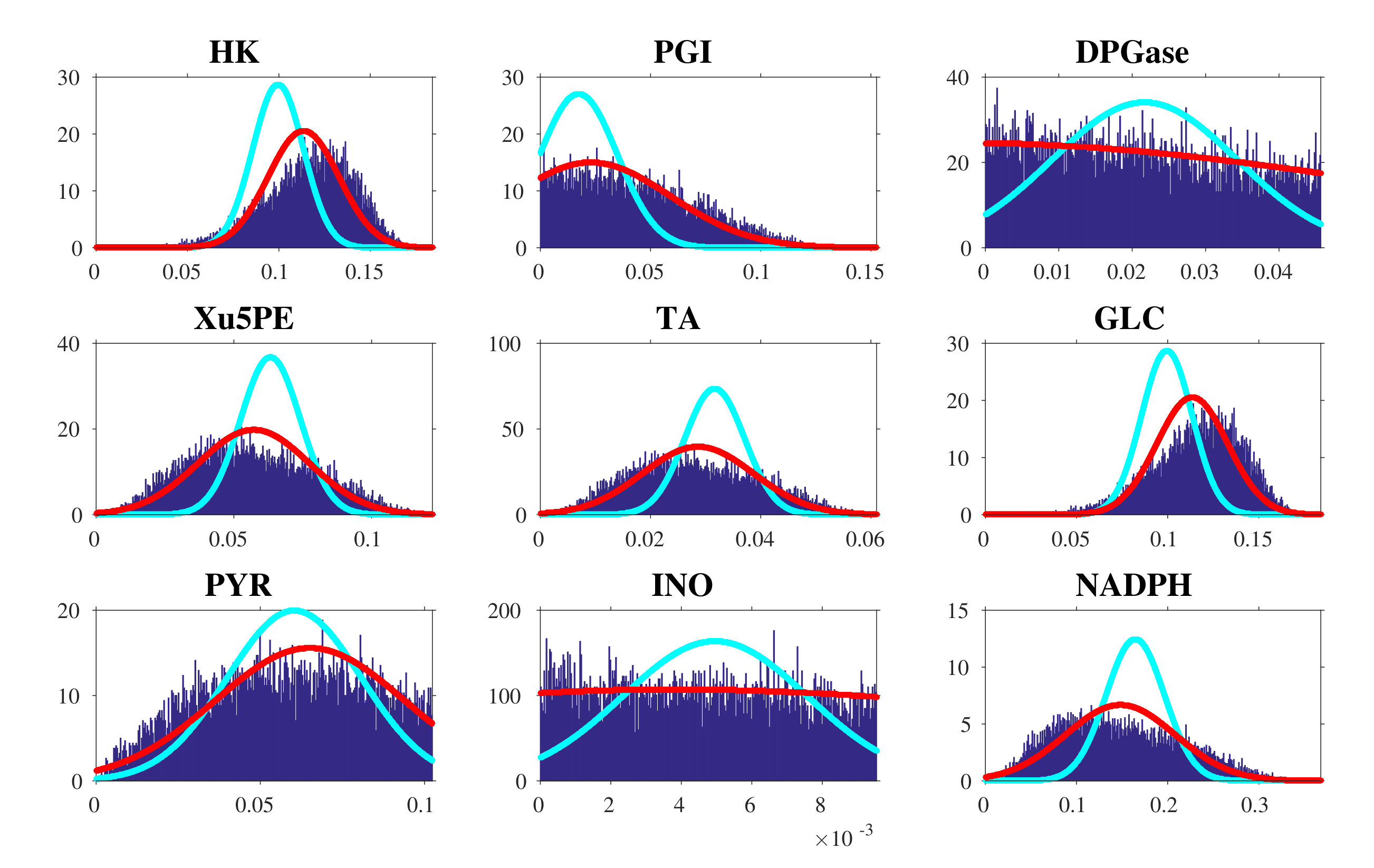 Figure 1
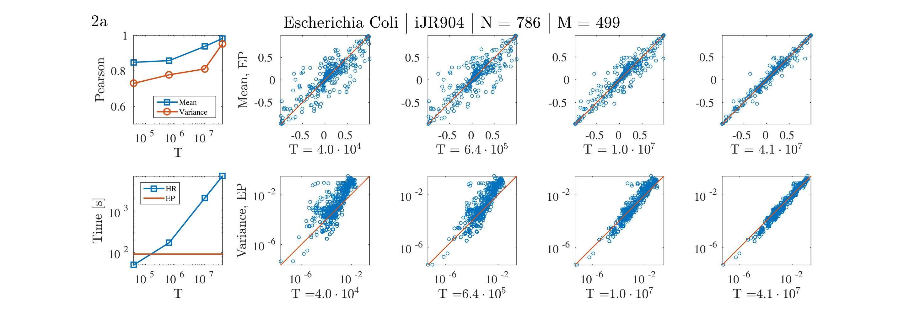 Figure 2
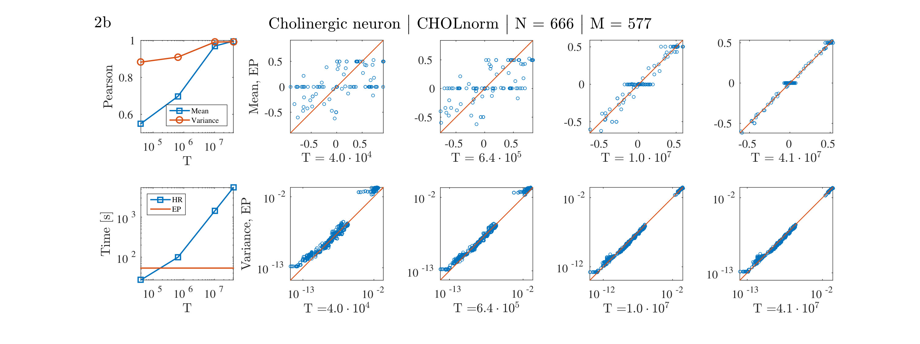 Figure 2
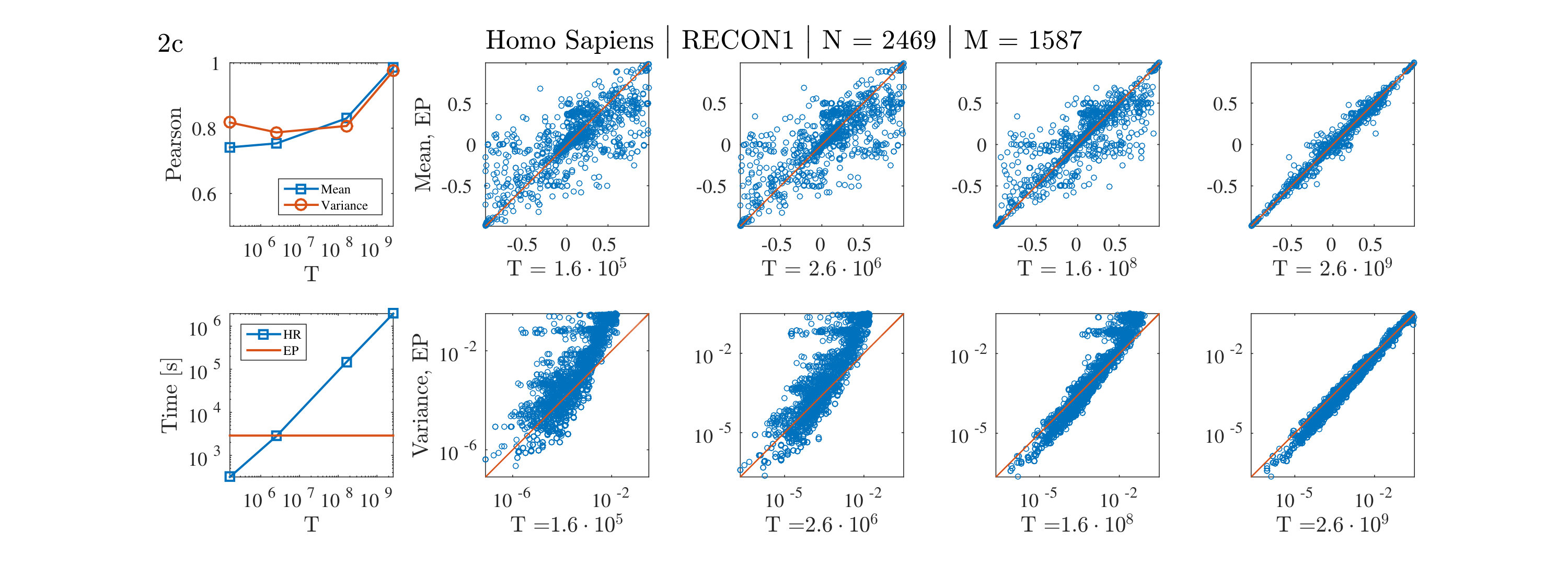 Figure 2
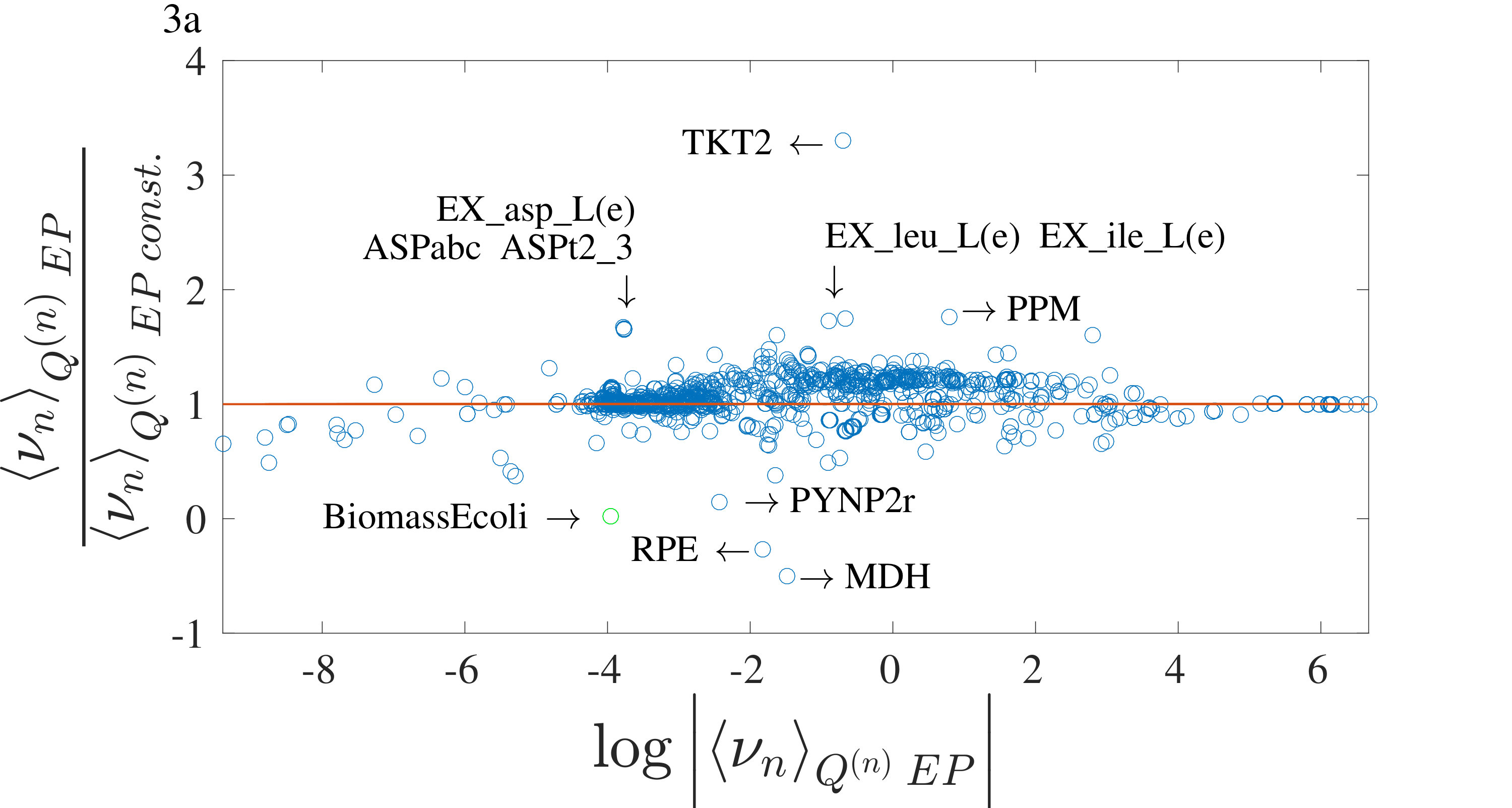 Figure 3
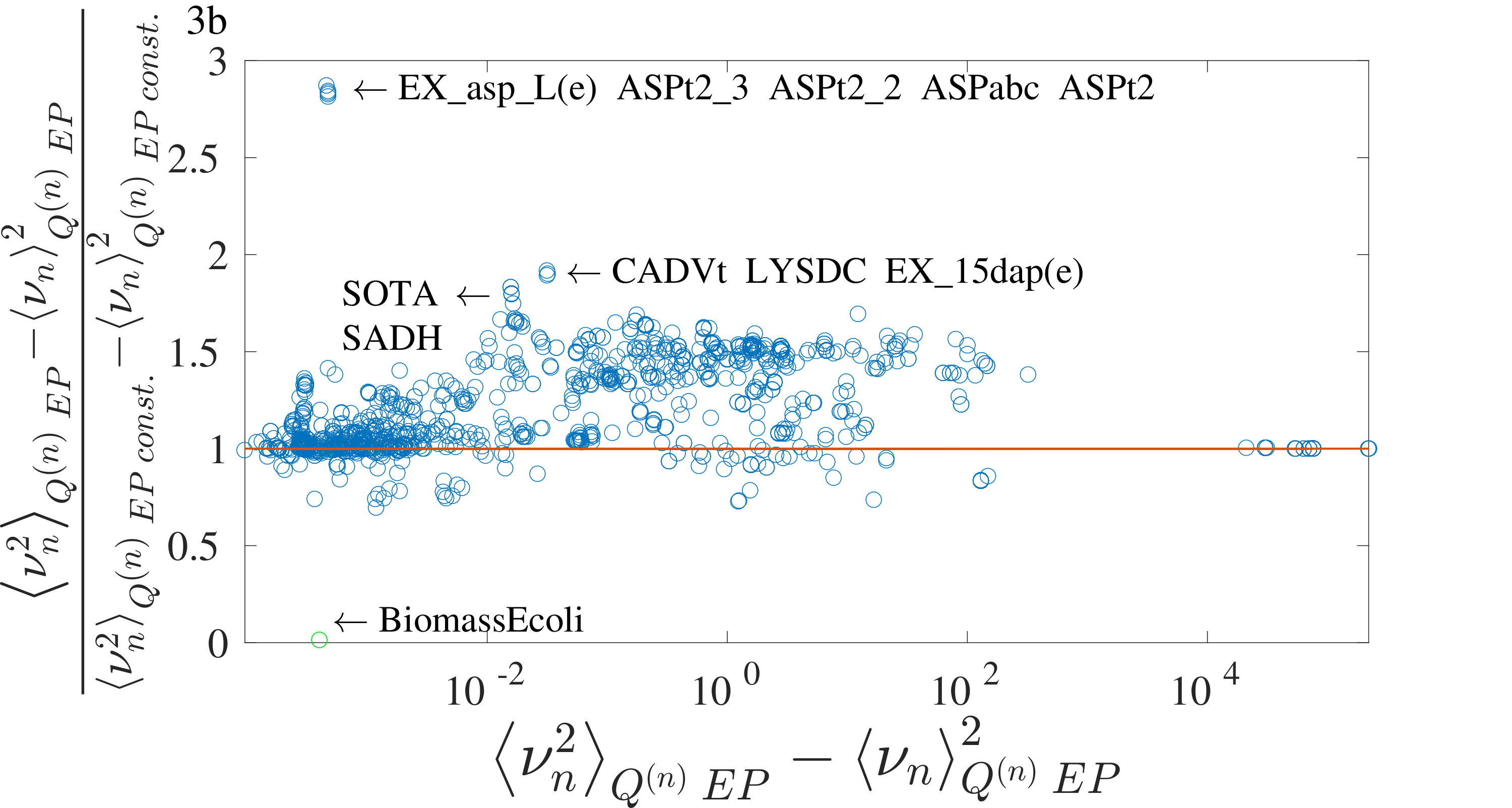 Figure 3
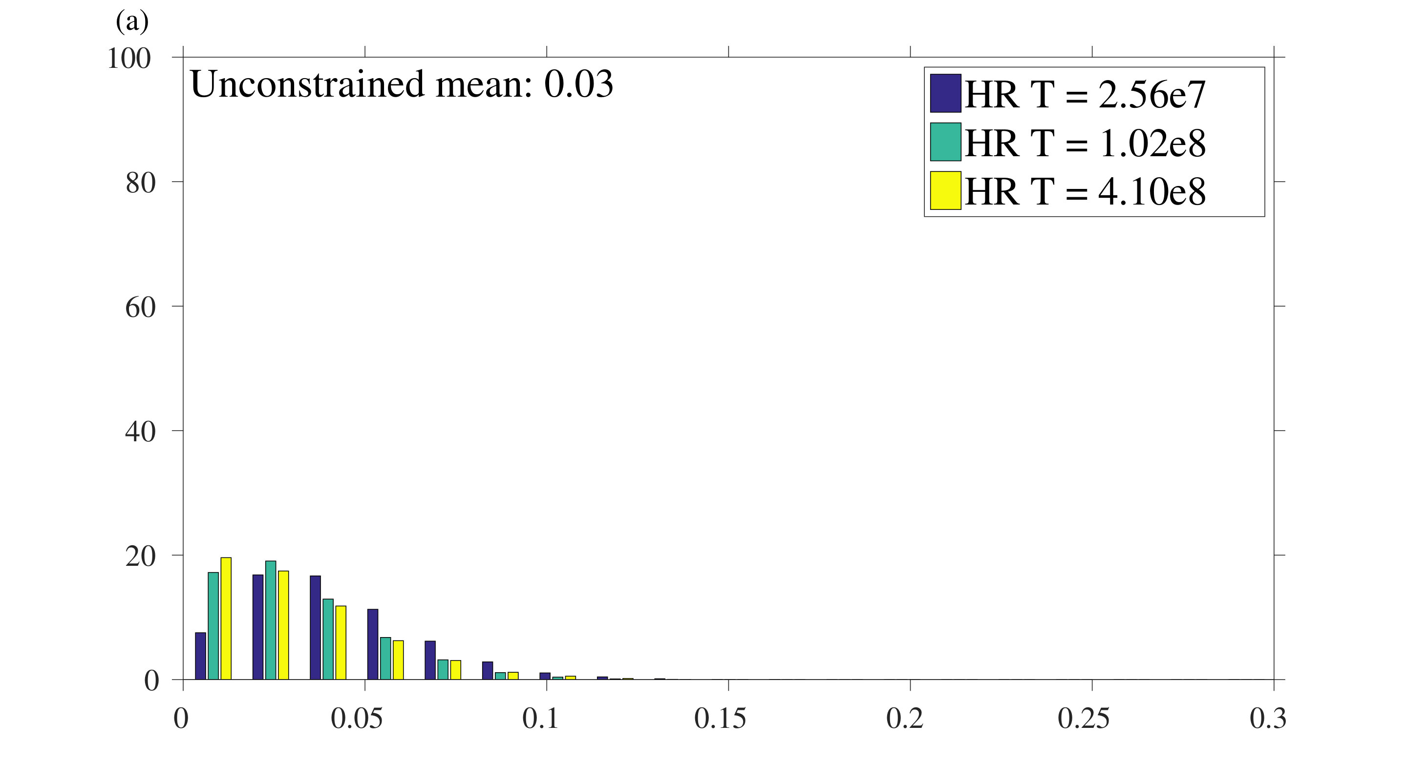 Figure 7
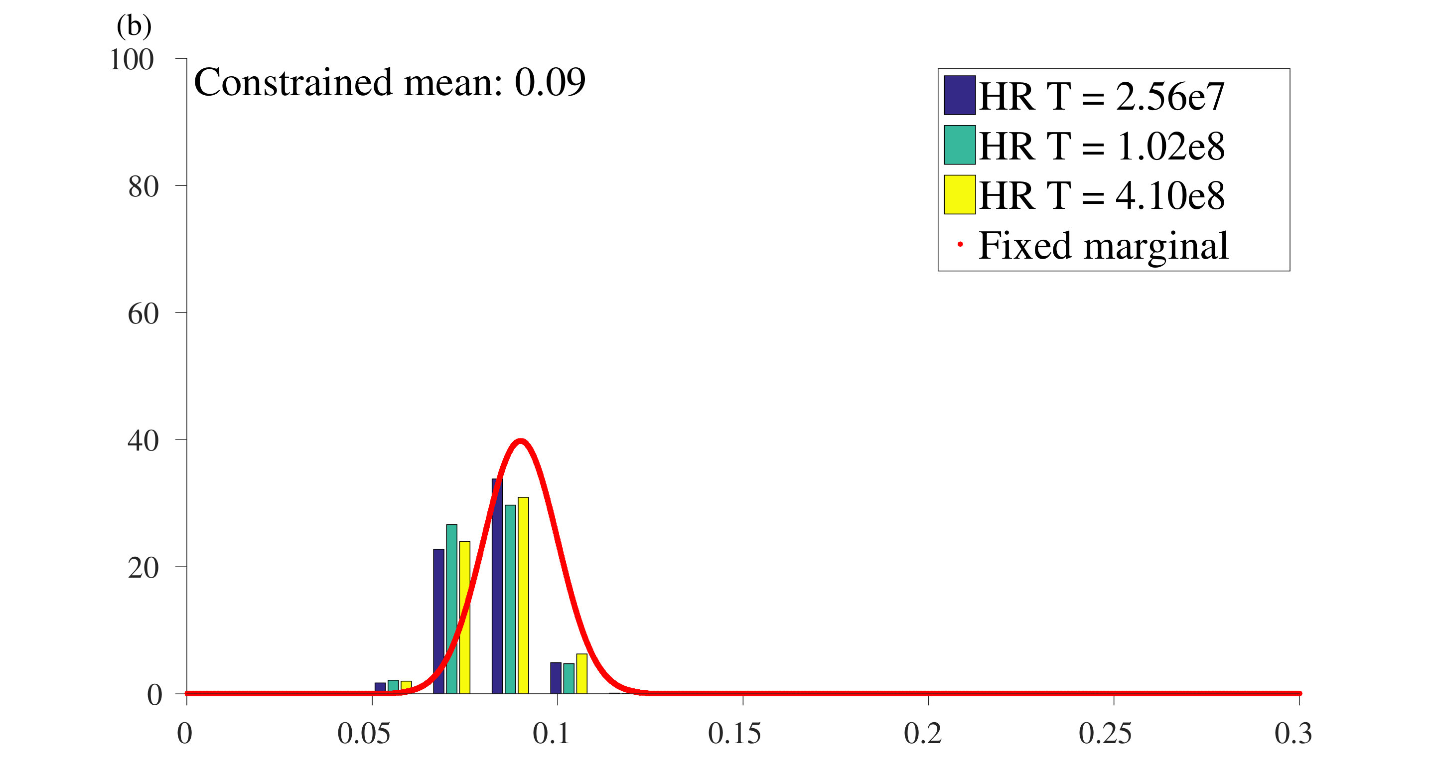 Figure 8
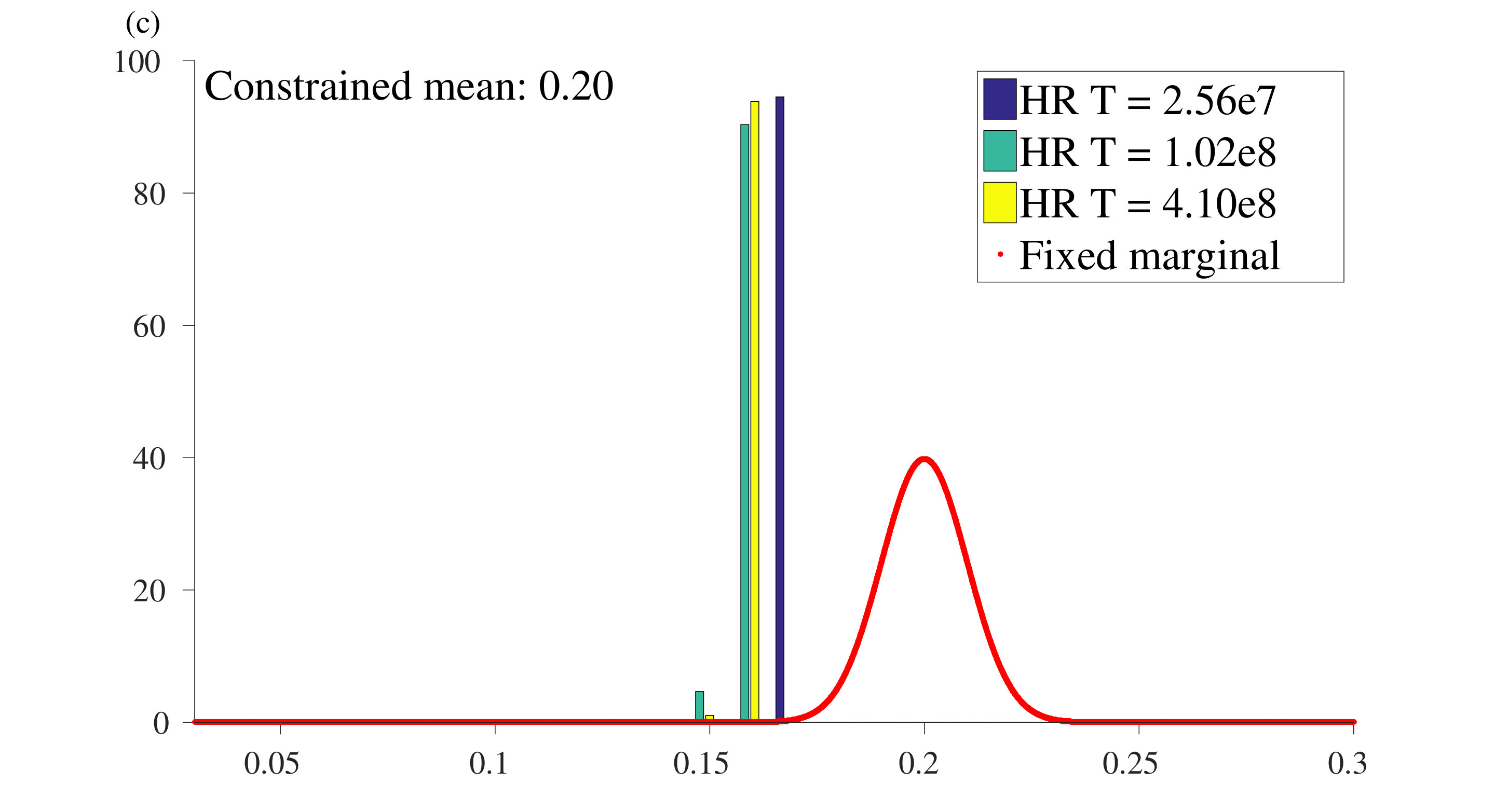 Figure 9
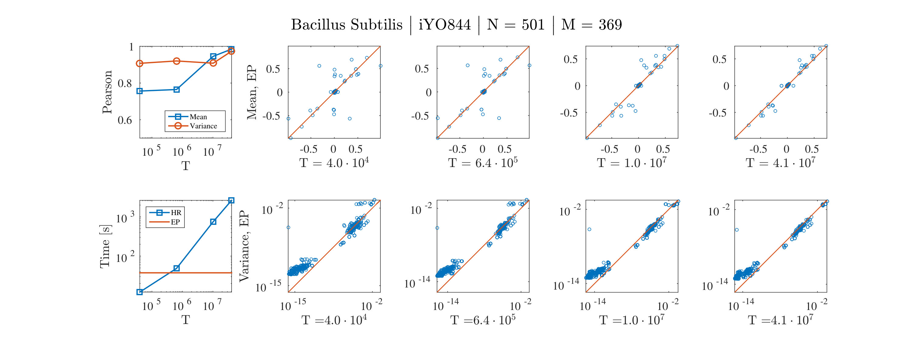 Figure 10
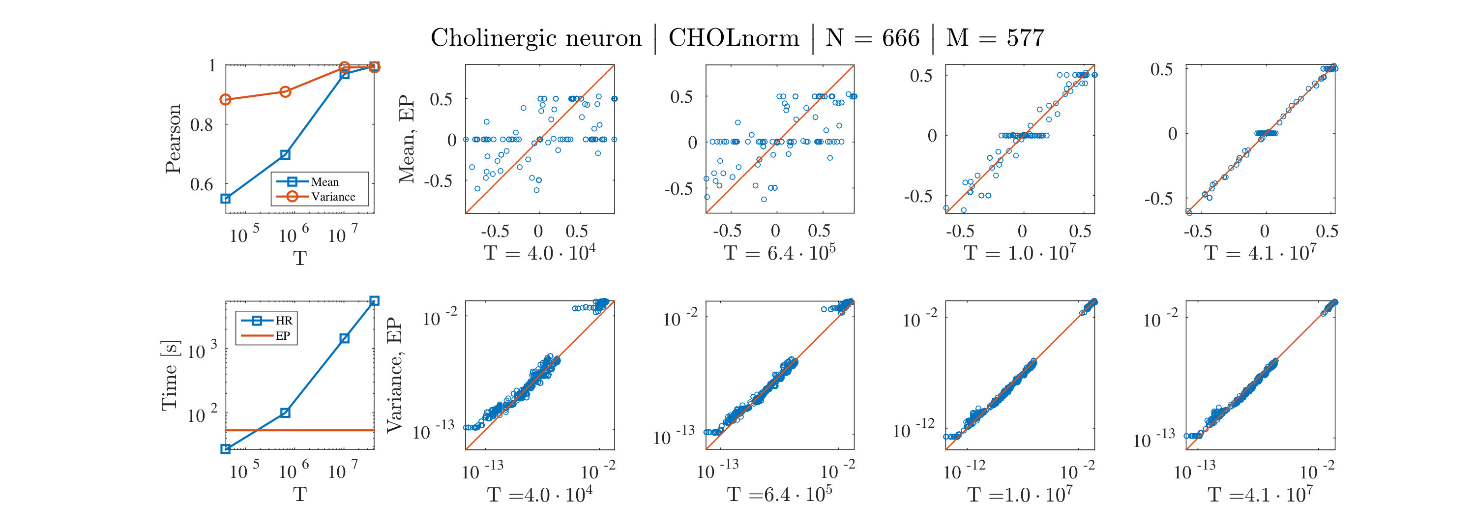 Figure 11
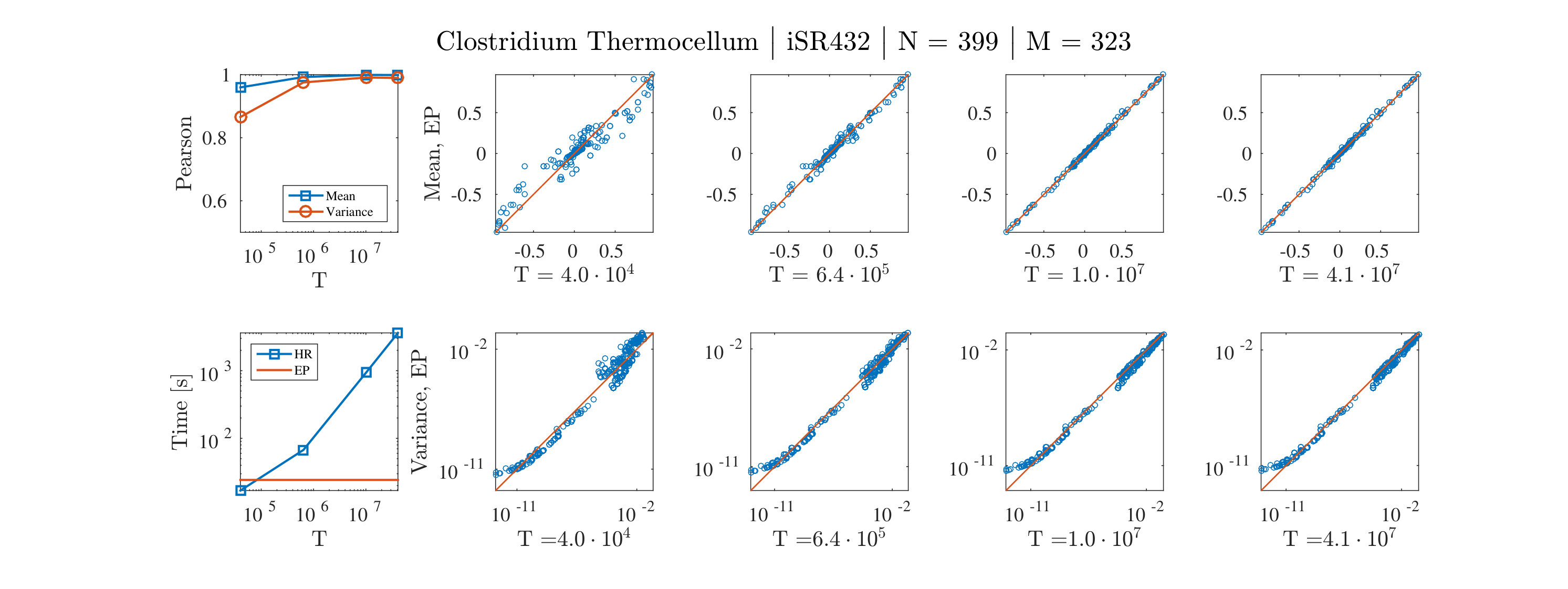 Figure 12
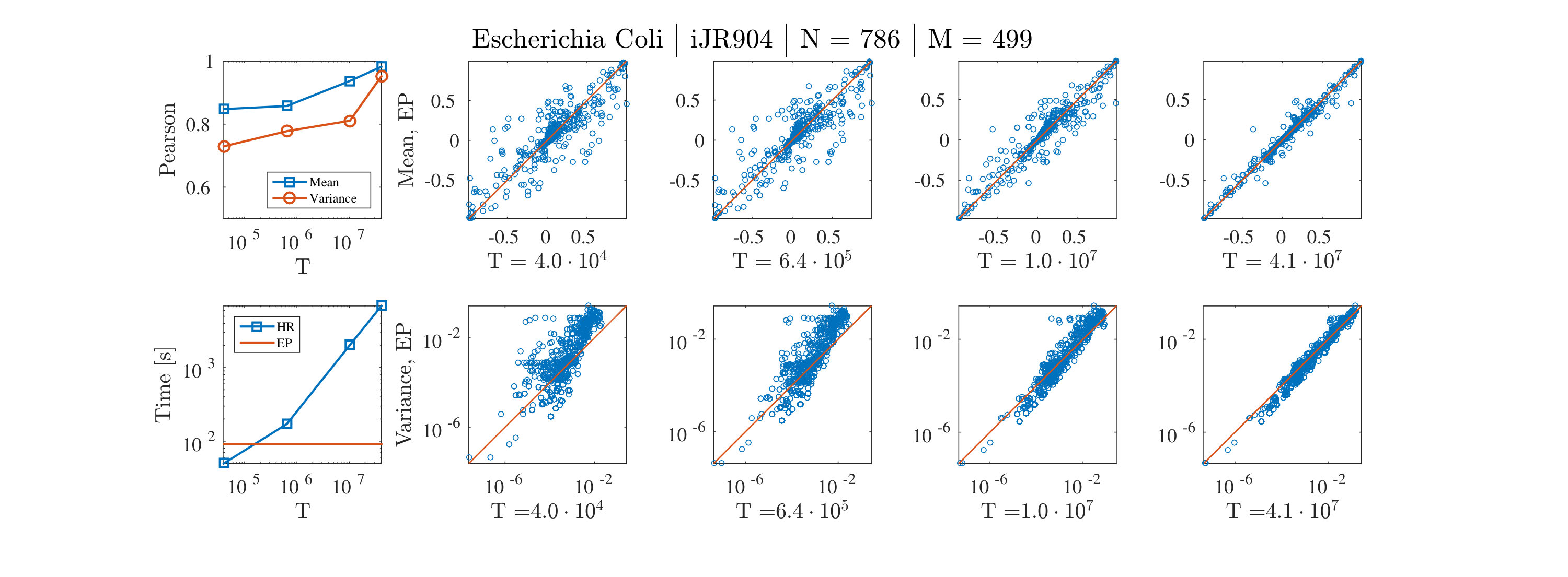 Figure 13
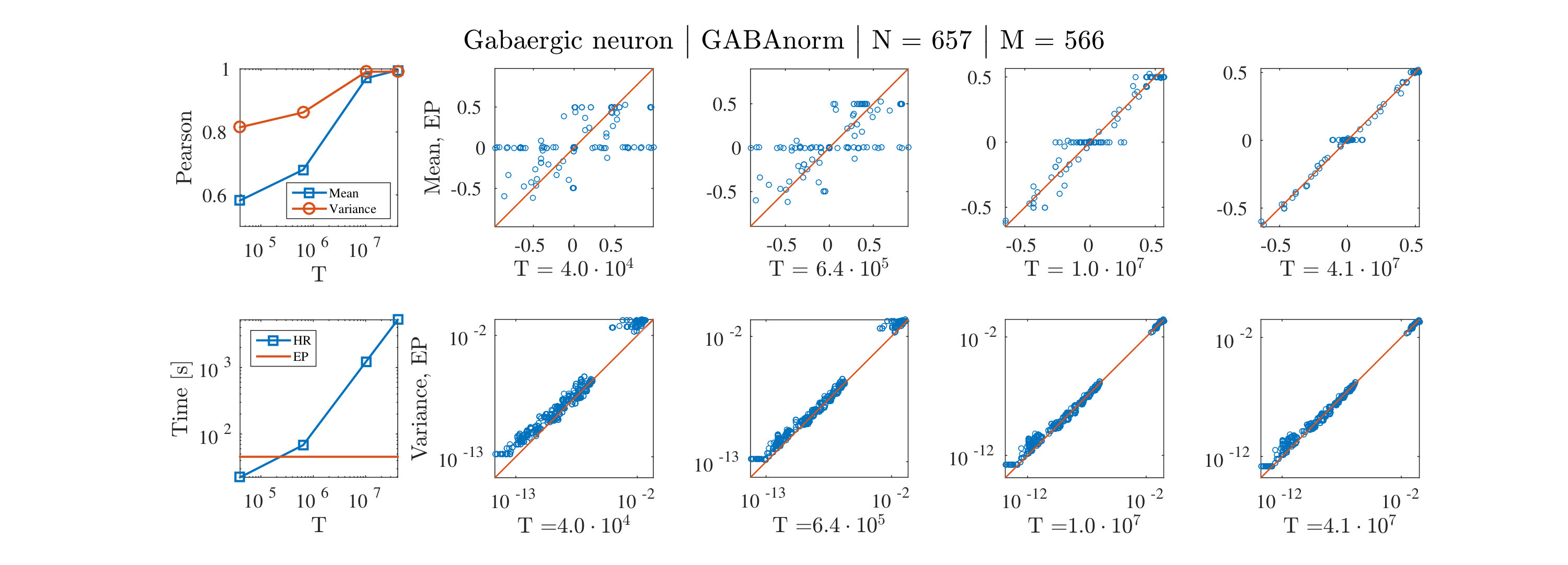 Figure 14
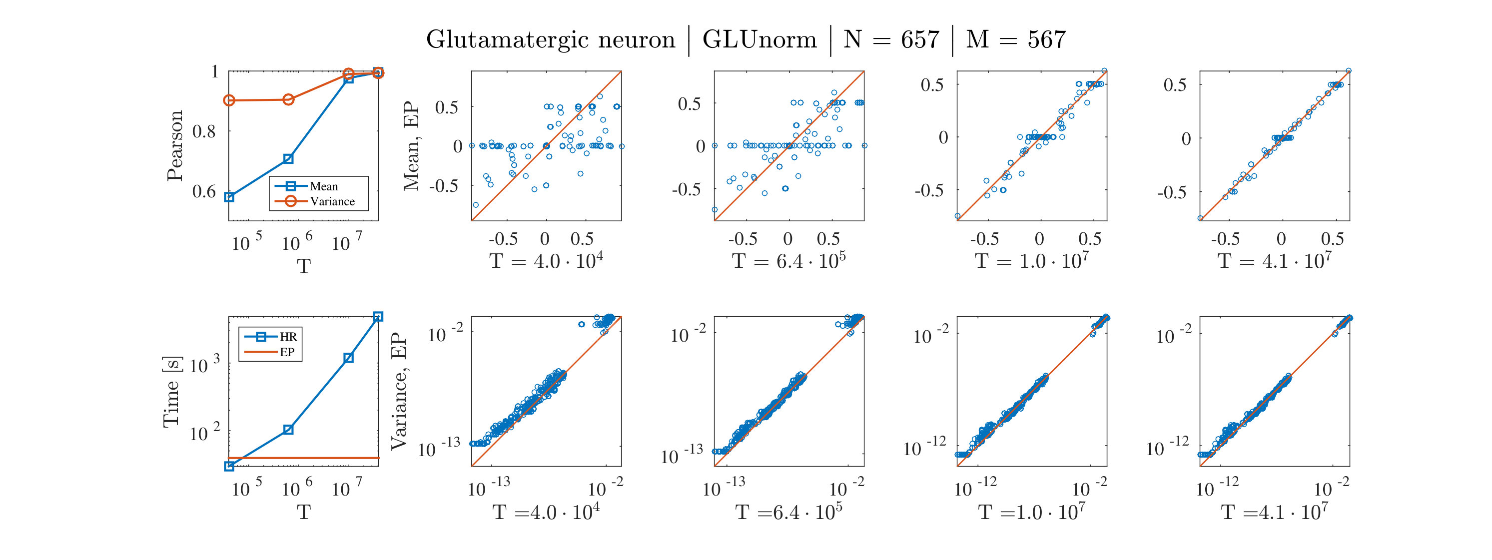 Figure 15
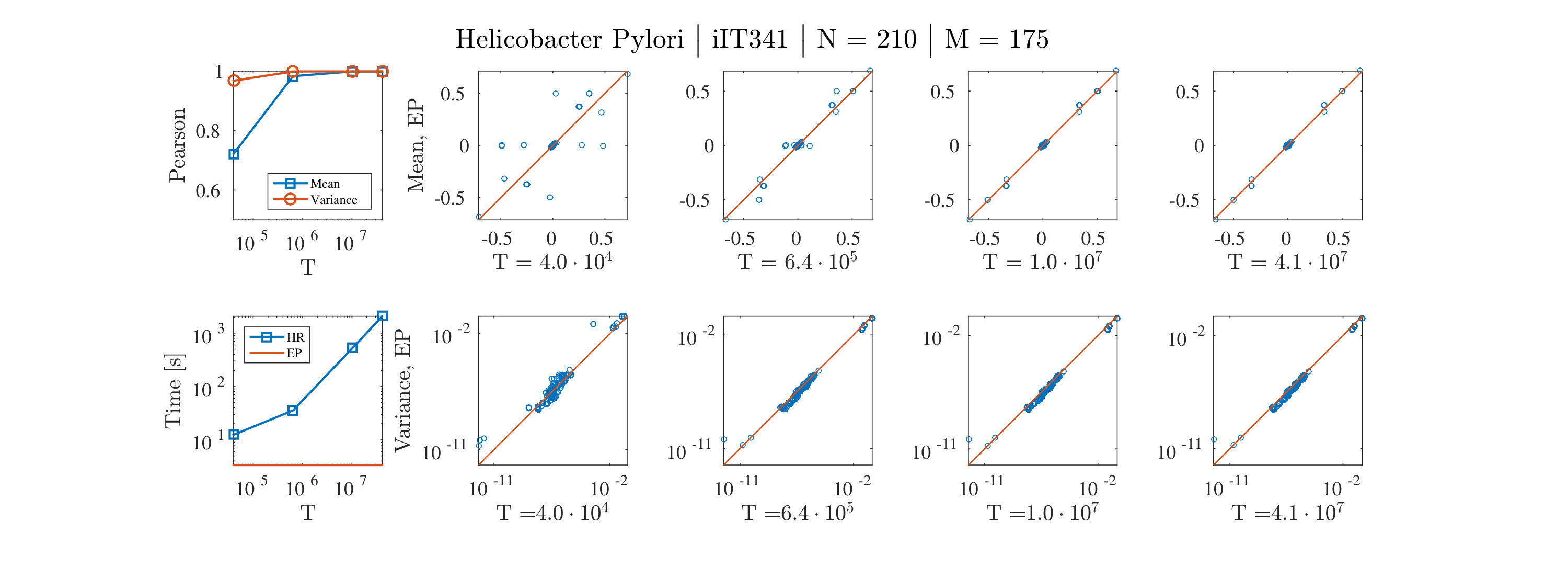 Figure 16
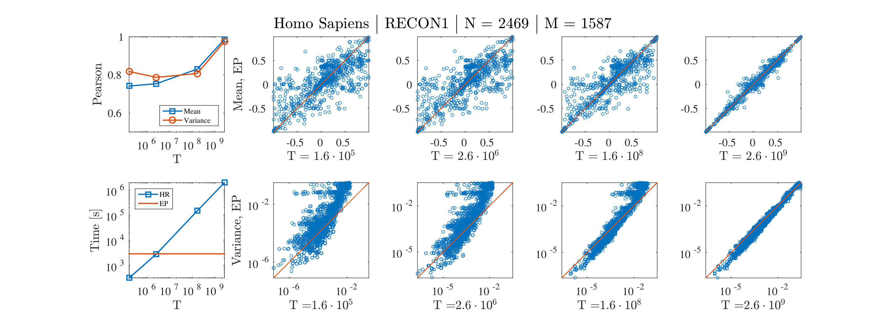 Figure 17
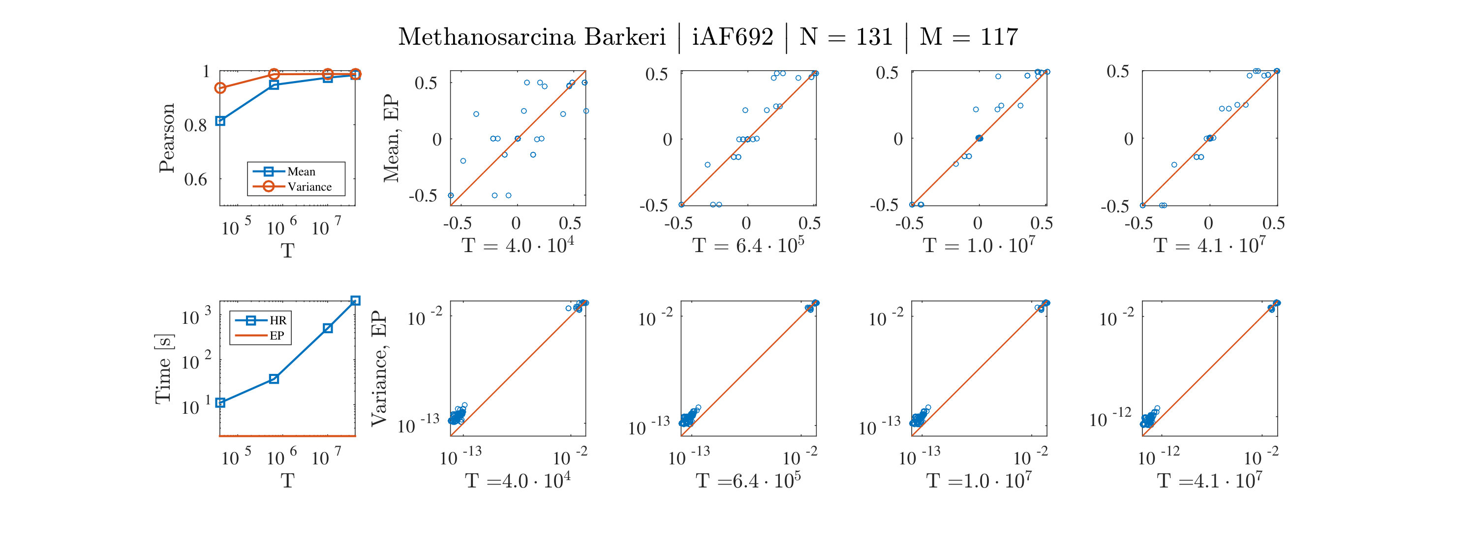 Figure 18
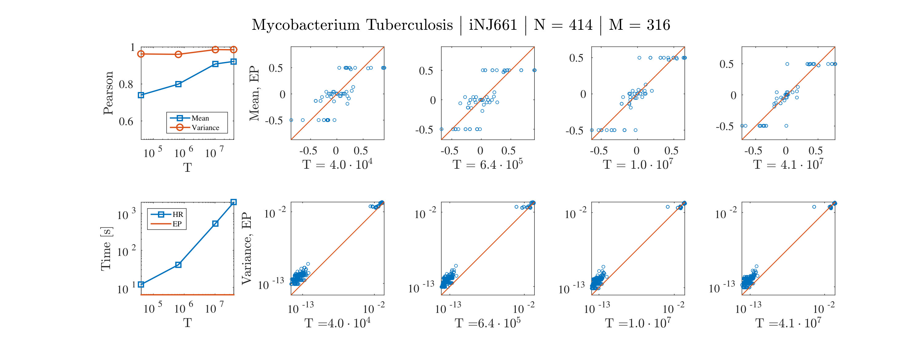 Figure 19
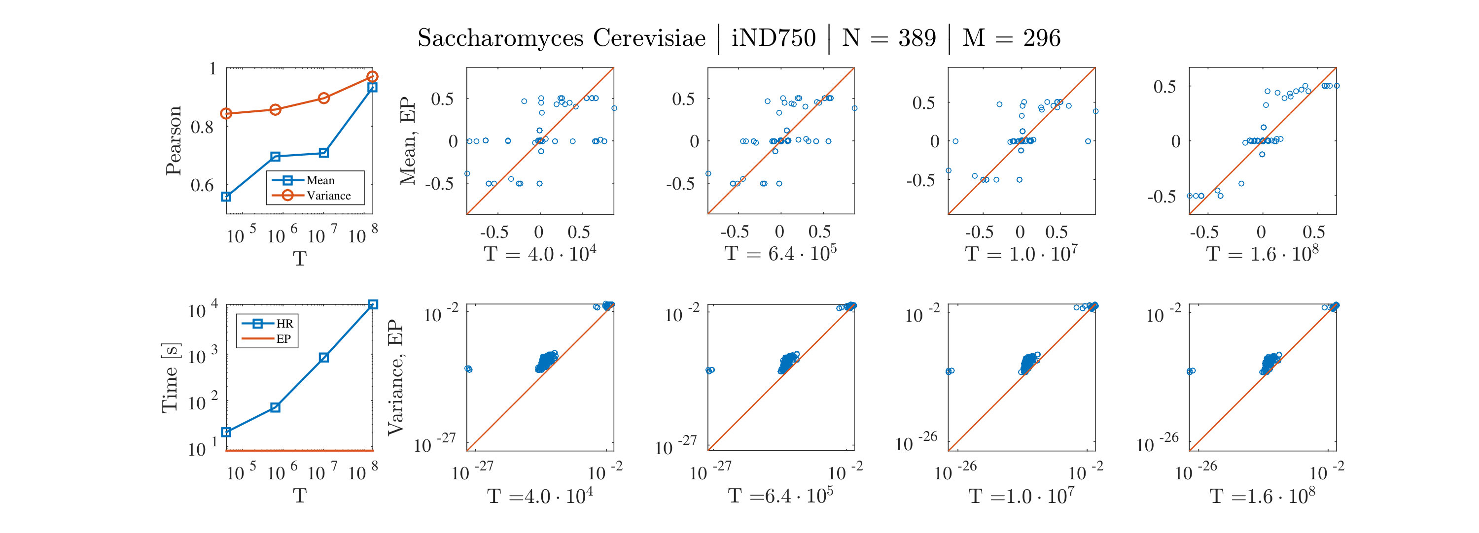 Figure 20
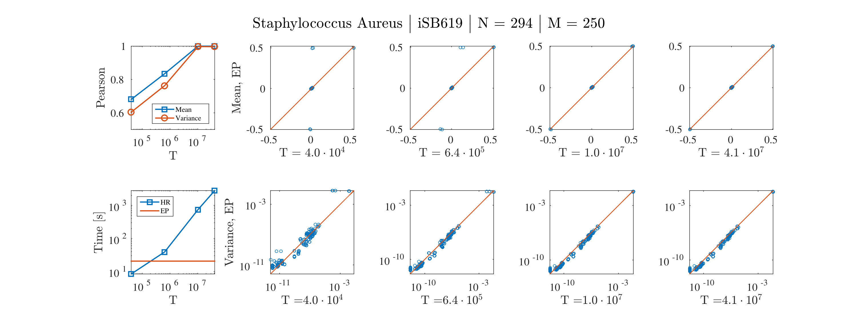 Figure 21
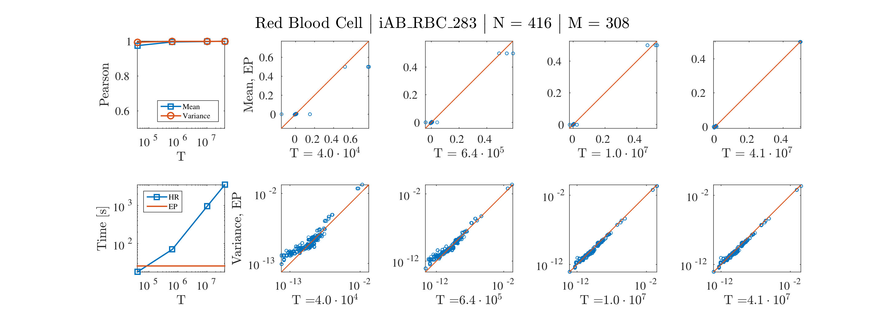 Figure 22
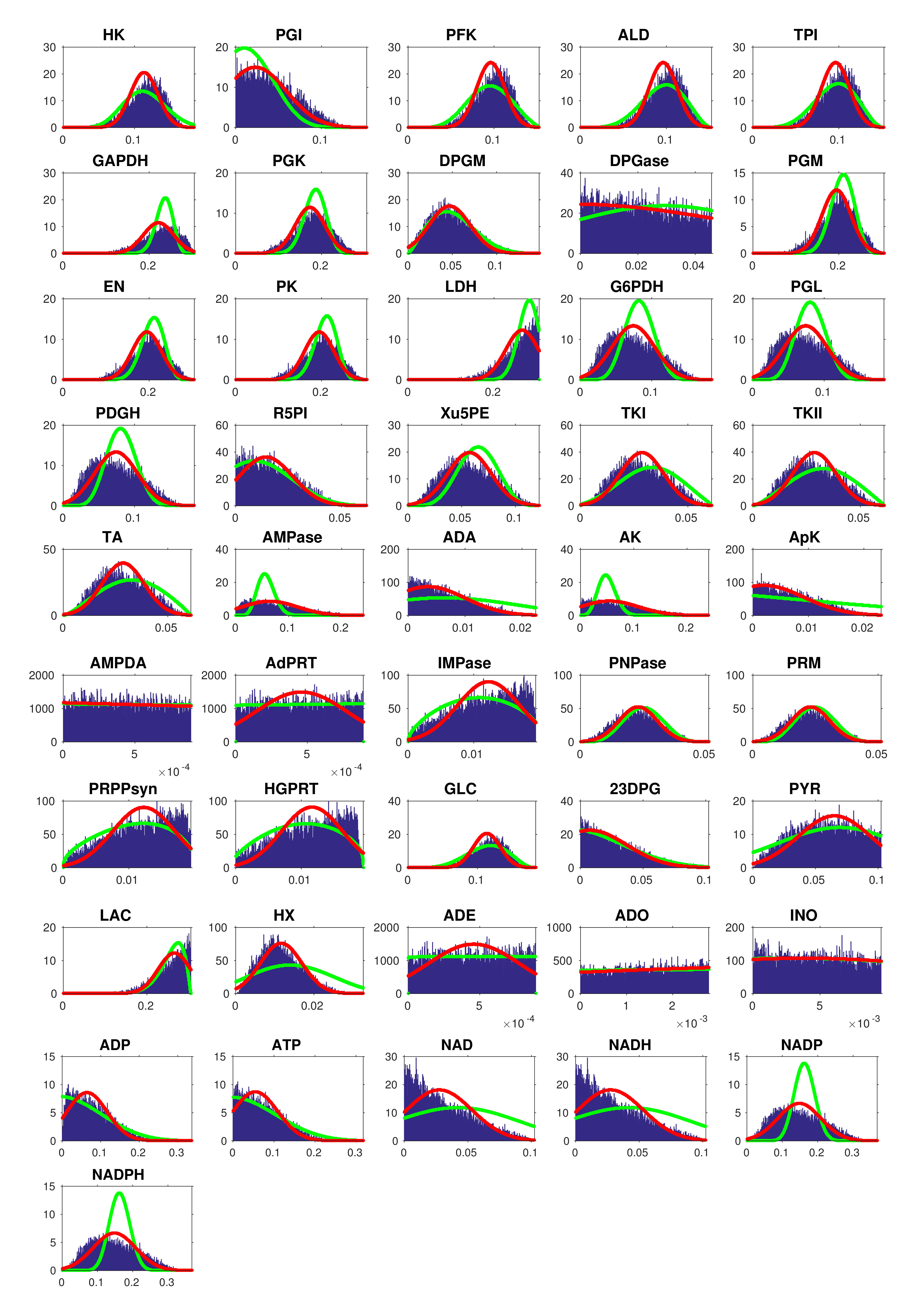 Figure 23
Peer Reviews
No public reviews on file for this paper yet. If you reviewed it on a platform where reviews are public (OpenReview, ICLR, NeurIPS, ICML), you can paste yours below so the community can read it here.
Videos
No videos yet. Explain this paper in a talk, walkthrough, or lecture? Add one.
An analytic approximation of the feasible space of metabolic networks
Alfredo Braunstein
DISAT, Politecnico di Torino, 10129 Torino, Italy
Human Genetics Foundation-Torino, 10126 Torino, Italy
Collegio Carlo Alberto, 10024 Moncalieri, Italy
Anna Paola Muntoni
DISAT, Politecnico di Torino, 10129 Torino, Italy
Andrea Pagnani
DISAT, Politecnico di Torino, 10129 Torino, Italy
Human Genetics Foundation-Torino, 10126 Torino, Italy
Istituto Nazionale di Fisica Nucleare (INFN) Via Pietro Giuria, 10125, Torino, Italy
Abstract
Assuming a steady-state condition within a cell, metabolic fluxes satisfy an under-determined linear system of stoichiometric* *equations. Characterizing the space of fluxes that satisfy such equations along with given bounds (and possibly additional relevant constraints) is considered of utmost importance for the understanding of cellular metabolism. Extreme values for each individual flux can be computed with Linear Programming (as Flux Balance Analysis), and their marginal distributions can be approximately computed with Monte-Carlo sampling. Here we present an approximate analytic method for the latter task based on Expectation Propagation equations that does not involve sampling and can achieve much better predictions than other existing analytic methods. The method is iterative, and its computation time is dominated by one matrix inversion per iteration. With respect to sampling, we show through extensive simulation that it has some advantages including computation time, and the ability to efficiently fix empirically estimated distributions of fluxes.
Introduction
The metabolism of a cell entails a complex network of chemical reactions performed by thousands of enzymes that continuously process intake nutrients to allow for growth, replication, defense and other cellular tasks nelson2008lehninger . Thanks to the new high-throughput techniques and comprehensive databases of chemical reactions, large scale reconstructions of organism-wide metabolic networks are nowadays available. Such reconstructions are believed to be accurate from a topological and stoichiometric viewpoint (e.g. the set of metabolites targeted by each enzyme, and their stoichiometric ratio). For the determination of reaction rates, large-scale constraint based approaches have been proposed palsson2015systems . Typically, such methods assume a steady-state regime in the system where metabolite concentrations remain constant over time (mass-balance condition). A second type of constraints limit the reaction velocities and their direction. In full generality the topology of a metabolic network is described in terms of the chemical relations between the metabolites and reactions. In mathematical terms we can define a stoichiometric matrix in which rows correspond to the stoichiometric coefficients of the corresponding metabolites in all reactions. A positive (resp. negative) term indicates that metabolite is created (resp. consumed) by reaction . Assuming mass-balance and limited interval of variation for the different reactions, we can cast the problem in terms of finding the set of fluxes compatible with the following linear system of constraints and inequalities:
[TABLE]
where is the known set of intakes/uptakes, and the pair represent the extremes of variability for the variables of our problem. Only in few cases the extremes are experimentally accessible, in the remaining ones they are fixed to arbitrarily large values. It turns out that , and the system is typically under-determined. As an example, the RECON1 model of Homo Sapiens has fluxes (*i.e. *variables) and metabolites (*i.e. *equations). The mass-balance constraints and the flux inequalities encoded in Eqs. (1)-(2) define a convex bounded polytope, which constitutes the space of all feasible solutions of our metabolic system.
The most widely used technique to analyze fluxes in large scale metabolic reconstruction is Flux Balance Analysis (FBA) varma_metabolic_1994 ; kauffman_advances_2003 where a linear objective function, typically the biomass or some biological proxy of it is introduced, and the problem reduces to find the subspace of the polytope which optimizes the objective function. If this subspace consists in only one point, the problem can be efficiently solved using linear programming. FBA has been successfully applied in many metabolic models to predict specific phenotypes under specific growth condition (e.g. bacteria in the exponential growth phase). However, if one is interested in describing more general growth conditions, or is interested in other fluxes than the biomass Suthers2007 , different computational strategies must be envisaged Marchiori_2014 ; fernandez-de-cossio-diaz_fast_2016 ; DeMartinoParisi2014 .
As long as no prior knowledge is considered, each point of the polytope is an equally viable metabolic phenotype of the biological system under investigation. Therefore, being able to sample high-dimensional polytopes becomes a theoretical problem with concrete practical applications. From a theoretical standpoint the problem is known to be #P-hard Dyer_Frieze1988 and thus an approximate solution to the problem must be sought. A first class of Monte Carlo Markov chain sampling techniques available to analyze large-dimensional polytopes was originally proposed three decades ago Smith1984 and falls under the name of Hit-and-Run (HR) turchin_computation_1971 . Basically, it consists on iteratively collecting samples by choosing random directions from a starting point belonging to the polytope. Unfortunately polytopes defined by large-scale metabolic reconstructions are typically ill-conditioned (i.e. some direction of the space are far more elongated than others), and improved HR techniques to overcome this problem have been proposed kaufman1998 and implemented in the context of metabolic modeling Schellenberger2011 ; Marchiori_2014 ; DeMartinoParisi2014 . Despite the fact that these dynamic sampling strategies are often referred as uniform random samplers, the uniformity of the sampling is guaranteed only in an asymptotic sense, and often establishing in practice how long a simulation should be run and how frequently the measurement should be taken for a given instance of the problem requires extensive preliminary simulations which make their use very difficult under general conditions. Note also that the problem of assessing how perturbations of network parameters affect the structure of the polytope is often of practical importance; e.g. changing extremal flux values for studying growth rate curves or enzymopaties Price2004 . In these situations in principle the convergence time of the algorithm should be established independently for each new value of the parameter. Another limitation of this class of sampling strategies is the difficulty of imposing other constraints schellenberger_use_2009 such as the experimentally measured distribution profiles of specific subset of fluxes (typically biomass and/or in-take/out-take of the network), a particularly timely issue given the recent breakthrough of metabolic measurements in single cell TaheriAraghi2015 , although recent attempts in this direction** **exist de_martino_scalable_2012 ; de_martino_growth_2016 .
Recently, alternative statistical methods based on message passing (MP) techniques (also known as cavity or Bethe approximation in the context of statistical mechanics) Mezard_Montanari_book have been proposed braunstein_estimating_2008 ; braunstein_space_2008 ; massucci2013 ; fernandez-de-cossio-diaz_fast_2016 ; font-clos_weighted_2012 , allowing for sampling of the polytope orders of magnitude faster than HR methods, under two main conditions: (i) the graphical structure of the graph must be a tree or, at least, locally tree-like (i.e. without short loops), (ii) the rows of the stoichiometric matrix should be statistically uncorrelated. Unfortunately, neither assumption is really fulfilled by large-scale metabolic reconstructions. To give an example, consider the rows of the stoichiometric matrix for ecoli-core model orth_reconstruction_2010 . The rows corresponding to the adenosine-diphosphate (ADP) and adenosine-triphosphate (ATP) appear strongly correlated as both metabolites commonly appear in 11 reactions; the same apply for the intracellular water and hydrogen ion that have 10 reactions in common. For these reasons MP methods suffer from all kind of convergence and accuracy problems.
In this work we propose a new Bayesian inference strategy to analyze with unprecedented efficiency large dimensional polytopes. The use of a Bayesian framework allows us to map the original problem of sampling the feasible space of solutions of Eqs. (1)-(2) into the inference problem of the joint distribution of metabolic fluxes. Linear and inequality constraints will be encoded within the likelihood and the prior probabilities that via Bayes theorem provide a model for the posterior . The goal of this work is to determine a tractable multivariate probability density able to accurately approximate the posterior even in the case of strongly row-correlated stoichiometric matrices. This strategy relies on an iterative and local refinement of the parameters of that falls into the class of Expectation Propagation (EP) algorithms. We report results of EP for representative state-of-the-art models of metabolic networks in comparison with HR estimate, showing that EP can be used to compute marginals in a fraction of the computing time needed by HR. We also show how the technique can be efficiently adapted to incorporate the estimated growth rate of a population of Escherichia Coli.
Results
Formulation of the problem
We are going to formulate an iterative strategy to solve the problem of finding a multivariate probability measure over the set of fluxes compatible with Eqs. (1)-(2). For a vector of fluxes satisfying bounds 2, we can define a quadratic energy function whose minimum(s) lies on the assignment of variables satisfying the stoichiometric constraints in Eq. (1):
[TABLE]
We define the likelihood of observing given a set of fluxes as a Boltzmann distribution:
[TABLE]
where is a positive parameter, the “inverse temperature” in statistical physics jargon, that governs the penalty of whose configurations of fluxes that are far from the minimum of the energy. In a Bayesian perspective one can consider the posterior probability of observing as:
[TABLE]
where the prior
[TABLE]
enforces the bounds over the allowed range of fluxes. The function is an indicator function that takes value if and [math] otherwise. We finally obtain the following relation for the posterior:
[TABLE]
and eventually we will investigate the limit. Neglecting terms that do not depend on , the posterior takes the form of
[TABLE]
where we have not explicitly reported the normalization constant. By marginalization of Eq. (7) one can determine the marginal posterior for each flux . However, performing this computation naively would require the calculation of a multiple integral that is in principle computationally very expensive and cannot be performed analytically in an efficient way.
A standard way of approximately computing is through sampling methods, such as the HR technique. The accuracy obtained with HR depends of course on the number of samples, and sampling accurately can be very time consuming. In the following we develop an analytic approach to approximately compute marginal posteriors which is able to achieve results as accurate as the HR sampling technique for a large number of sampled points in a fraction of the computing time. But first, we will describe as a warm-up a naive analytic method to approximately compute marginal distributions .
A non-adaptive approach
As a first approximation one can think of replacing each exact prior with a single Gaussian distribution whose statistics, i.e. the mean and the variance, are constrained to be equal to the one of . That is
[TABLE]
We estimate the marginal posteriors from the distribution
[TABLE]
Notice that in this approximation fluxes result unbounded. Marginals obtained by this strategy against the Hit-and-Run Monte Carlo estimate are shown is Figure 1 (cyan line) for 9 representative metabolic fluxes of one of the standard model for red blood cell wiback_monte_2004 . Marginals evaluated with this simple non-adaptive strategy differ significantly from the ones evaluated with the Montecarlo sampling technique. In the following we will show how we can overcome this limitation by choosing different values for the means and the variances in Eq. 10 making use of the Expectation Propagation algorithm.
Expectation Propagation
Expectation Propagation (EP) minka_expectation_2001 is an efficient technique to approximate intractable (i.e. impossible or impractical to compute analytically) posterior probabilities. EP was first introduced in the framework of statistical physics as an advanced mean-field method opper_gaussian_2000 ; opper_adaptive_2001 and further developed for Bayesian inference problems in the seminal work of Minka minka_expectation_2001 .
Let us consider the flux and its corresponding approximate prior . We define a tilted distribution as
[TABLE]
The important difference between the tilted distribution and the multivariate Gaussian is that all the intractable priors are approximated as Gaussian probability densities except for the prior which is treated exactly. For this reason we expect that this distribution will be more accurate than regarding the estimate of the statistics of flux without significantly affecting the computation of expectations. Bearing in mind that it is a large number of *exact *priors (i.e. the distributions ) that make the computation intractable and not a single one, we have introduced only one exact intractable prior in .
One way of determining the unknown parameters and of is to require that the multivariate Gaussian distribution is as close as possible to the auxiliary distribution . Intuitively, there are at least two possibilities to enforce this similarity: (i) matching the first and the second moments of the two distributions (ii) minimizing the Kullback-Leibler divergence ; these two methods coincide (see details in Supplementary Note 1). Thus, we aim at imposing the following moment matching conditions:
[TABLE]
from which we get a relation for the parameters , that is explicitly reported in Section Update rule.
EP consists in sequentially repeating this update step for all the other fluxes and iterate until we reach a numerical convergence. Further technical details about the convergence are reported in Subsection Numerical results for large scale metabolic networks. At the fixed point we directly estimate the marginal posteriors , for , from marginalization of the tilted distribution that turns out to be a truncated Gaussian density in the interval (see Supplementary Note 2).
At difference from the non-adaptive approach, the EP algorithm determines the approximated prior density by trying to reproduce the effect that the true prior density has on variable , including the interaction of this term with the rest of the system. First, the information encoded in the stoichiometric matrix is surely encompassed in the computation of the means and the variances of the approximation since both the distributions and contain the exact expression of the likelihood. Secondly, the refinement of each prior also depends on the parameters of all the other fluxes.
As an example of the accuracy of this technique we report in Figure 1 (red line) the nine best marginals estimated by EP of the red blood cell against the results of Hit-and-Run Monte Carlo sampling. Fig. 1 suggests that this technique leads to a significant improvement of the non-adaptive approximation as the plot shows a very good overlap between the distributions provided by HR and EP. The entire set of marginals and a comparison with a state-of-the-art message passing algorithm fernandez-de-cossio-diaz_fast_2016 is reported in the Supplementary Fig. 2.
Numerical results for large scale metabolic networks
This section is devoted to compare the results of our algorithm against the outcomes of a state-of-the-art Hit-and-Run Monte Carlo sampling technique on three representative models of metabolic networks, precisely the iJR904 reed_expanded_2003-1 , the CHOLnorm lewis_large-scale_2010 and the RECON1 duarte_global_2007 models for Escherichia Coli, the Cholinergic neuron and Homo Sapiens organisms respectively. In Supplementary Fig. 3 we report results for a larger set of models all selected from the Bigg Models database king2016bigg .
Experiments are performed as follows. First we preprocess the stoichiometric matrix of the model in order to remove all reactions involving metabolites that are only produced or only degradedhenry2010high .
After the pre-processing, we run HR and EP, both implemented on Matlab or as Matlab libraries, to the reduced model. Let us explain how the two methods work. Starting from a point lying on the polytope, HR iteratively chooses a random direction and collects new samples in that direction such that they also reside in the solution space. In this work we use an optimized implementation of HR, called optGpSampler Marchiori_2014 . Regarding the HR simulations we set the number of sampled points to be equal to for an increasing number of explored configurations from to in most of the cases; for some specific models, i.e. very large networks having reactions, we explore up to points. Concerning the EP algorithm we perform the same experiment setting the parameter to be equal to for almost all models. In only one case (the RECON1 model), we encountered convergence problems and thus we decreased it to . Numerical convergence of EP depends on the refinement of parameters and or, more precisely, on the estimate of the marginal distributions of fluxes. At each iteration we compute an error which measures how the approximate marginal distributions change in two consecutive iterations. Formally, we define the error as the maximum value of the sum of the differences (in absolute values) of the mean and second moment of the marginal distribution, that is
[TABLE]
If is smaller than a predetermined target precision (we used , the algorithm stops.
To quantitatively compare the two techniques we report here the scatter plots of variances and means of the approximate marginals computed via HR and EP. Moreover we estimate the degree of correlation among the two sets of parameters computing the Pearson product-moment correlation coefficient
Notice that we cannot have access to the exact marginals and that we assume that the results obtained by HR are exact only asymptotically. Thus our performances, both for the direct comparison of the means and variances and for the Pearson’s coefficient, should be considered accurate if they are approached by the Monte-Carlo ones for an increasing number of explored points.
The three large subplots in Fig. 2 show the results for Escherichia Coli, Cholinergic neuron and Homo Sapiens respectively. For each organism, we report on the top-left panel the time spent by EP (straight line) and by HR (cyan points) and on the bottom-left panel the Pearson correlation coefficients. Both measures of time and correlation, are plotted as functions of the number of configuration obtained from the HR algorithm. As shown in these plots, we can notice that to reach a high correlation regime a very large number of explored configurations, employing a computing time that is always several orders of magnitude larger than the EP running time. This is particularly strinking in the case of the RECON1 model, for which we needed to run HR for about 20 days in order to reach results similar to the outcomes of EP, that converges in less than one hour on the same machine.
To underline how EP seems to approach HR results in the asymptotic limit, we report in the rest of the sub-figures the scatter plots of the means (top) and the variances (bottom) of the marginals. On the -axis we plot the EP means (variances) against the HR means (variances) for an increasing number of explored configurations, as indicated in -axis. Results clearly show that as grows, the points (both means and variances) are more and more aligned to the identity line: not only these measures are highly correlated for large , but they assume very similar values. This is remarkably appreciable in the results for model: for the means of the scatter plots are quite unaligned but as reaches , they almost lie on the identity line. In fact, means are poorly correlated for while the Pearson correlation coefficient is close to 1 for .
Study of Escherichia Coli metabolism for a constrained growth rate
The EP formalism can efficiently deal with a slightly modified version of problem of sampling metabolic networks. Suppose to have access to experimental measurements of the distribution of some fluxes under specific environmental conditions. We would like to embed this empirical knowledge in our algorithm, by matching the posterior distribution of the measured fluxes with the empirical measurements. Within the EP scheme, this task corresponds to matching the first two moments (mean and variance) of the posteriors with the one defined by the empirical measurements. With the inclusion of empirically established prior knowledge, we want to investigate how the experimental evidence is related to the metabolism at the level of reactions or, in other words, we want to determine how fluxes modify in order to reproduce the experiments. In this perspective, the EP scheme can easily accommodate additional constraints on the posteriors by modifying the EP update equations as outlined in Methods.
We have tested this variant of EP algorithm on the iJR904 model of Escherichia Coli for a constrained growth rate. In fact, one of the few fluxes that are experimentally accessible is the biomass flux, often measured in terms of doubling per hour. As a matter of example we decide to extract one of the growth rates reported in Fig. 3(a) of PhysRevE.93.012408 ; the profile labeled as Glc (P5-ori) can be well fitted by a Gaussian probability density of mean and variance . This curve represent single-cell measures of a population of bacteria living in the so-called minimal substrate whose main characteristics are in principle well caught by the iJR904 model. We fixed the bound on the glucose exchange flux EX_glc(e) such that the maximum allowed growth rate (about ) contained all experimental values in the profile labeled as Glc (P5-ori) of Fig. 3(a) of PhysRevE.93.012408 . This was easily computed by fixing the biomass flux to the desired value and minimizing the glucose exchange flux using FBA, and gies a the lower bound of the exchanged glucose flux of .
We then apply EP algorithm to the modified iJR904 model in two different conditions. First, we do not impose any additional constraint and we run the original EP algorithm as described in the previous section. Then, as described in Methods, we fix the marginal posterior of the biomass. We can now compare the means and the variances of all the other fluxes in the two cases and single out those fluxes that have been more affected by the empirical constraints on the growth rate. We report in Fig. 3 the plot of the ratio between the means (Fig. 3 (a)) and the variances (Fig. 3 (b)) in the unconstrained case and in the constrained case. In Fig. 3 (a) these ratios are plotted against the logarithm of the absolute value of the unconstrained means to differentiate those fluxes having means close to zero and all the other cases. The ratios of the variances are instead plotted as a function of the unconstrained variances in semi-log scale. We can notice that apparently a large fraction of the fluxes have changed their marginal distribution in order to accommodate the fixed marginal for the biomass. We have reported the name of the reactions with the most significant changes; for instance, the marginal of the *TKT2 reaction has reduced its mean of more than one third, while many reactions involving aspartate *have significantly lowered their variances.
To underline the non-trivial results of EP algorithm in the constrained case, we apply again the standard EP algorithm to the iJR904 model when the lower bound and the upper bound of the biomass is fixed to the average value of the experimental profile. The comparison (not shown) between the two approaches suggests that the most relevant change concerns the EX_asp_L(e) flux as both the average value and the variance estimated in the second case are about two times the ones predicted by constrained EP. The distributions of most other fluxes remain do not considerably change. We underline that the different behavior of the marginals in the two cases, even if not significant for most of the fluxes, was in principle unpredictable without the use of constrained EP; and we do not exclude that fixing other empirical profiles can lead to very different results. Likewise, it seems unlikely that the results computed with constrained EP could be obtained using unbiased samples as provided by standard HR implementations (see a discussion in Supplementary Note 6).
Discussion
In this work we have shown how to study the space of feasible configurations of metabolic fluxes within a cell via an analytic description of the marginal probability distribution characterizing each flux. Such marginals are described as truncated Gaussian densities whose parameters are determined through an iterative and extremely efficient algorithm, the Expectation Propagation algorithm. We have compared our predictions against the estimates provided by HR sampling technique and results shown in Subsection Numerical results for large scale metabolic networks suggest a very good agreement between EP and HR for a large number of explored configurations, . First of all, the direct comparison of the means and variances of EP vs HR reported in the scatter plots shows that the more we increment the HR points, the more the scatter points are aligned. Secondly we see an increment of the correlation between EP and HR statistics for an increasing number of sampled points; correlations reach values very close to for large values of and for almost all the models we have considered. The most important point is that the computation times of EP, at high correlation regime, are always orders of magnitude lower than HR sampling times. This is extremely time-saving when we deal with very large networks, as the RECON1 model for Homo Sapiens where the running time (in seconds) of EP is three order of magnitude smaller then HR. We underline that exact marginals are generally inaccessible and we cannot compare our results against a ground-truth; our measures well approximate “true” distributions as long as the exactness of HR in the asymptotic limit is correct.
We have shown how to include empirical knowledge on distribution of fluxes on the EP algorithm without compromising the computing time. More precisely we have investigated how fixing an experimental profile of the growth rate into the iJR904 model of Escherichia Coli affect non-trivially all other fluxes. This is a remarkable advantage of the EP algorithm with respect to other methods.
EP provides an analytic estimate of each single flux marginal which relies on the optimization of two parameters, the mean and the variance of a Gaussian distribution. The formalism allows in principle more complicated parametrizations of posteriors to include other biological insights.
EP equations are extremely easy to derive and to implement, as the main loop can be written in few lines of Matlab code. The method is iterative, and the number of operations in each iteration scales as , rendering EP extremely convenient in terms of computation time with respect to existing alternatives.
An shown in Fig. 2 in real cases variances of the marginal distributions can span several orders of magnitude. This range of variability implies that also the variances of the approximation need to allow both very small and huge values. To cope with the numeric problems that may arise, we allow parameters to vary in a finite range of values with the drawback of limiting the set of allowed Gaussian densities of the approximation. For instance, a flat distribution cannot be perfectly approximated through a Gaussian whose variance cannot be arbitrary large; in the opposite extreme, imposing a lower bound on variances prevents the approximation of posteriors that are too concentrated on a single point. Thus this range needs to be reasonably designed in order to catch as many “true” variances as possible. In this work we have tried to impose a very large range of values, typically , to include as many distributions as possible without compromising the convergence of the algorithm. Moreover, the Gaussian profile itself is surely a limitation of the approximation as true marginals can have in principle arbitrary profiles.
EP performances are sensitive to the parameter and equations become numerically unstable for too large (e.g. ). On the other hand can be seen as the inverse-variance of a Gaussian noise affecting the conservation laws. The nature of this noise could depend on localization properties on the cell and real thermal noise. In this case, an optimization of the free energy with respect to can in principle lead to better predictions.
Methods
Update rule
The algorithm described in the Expectation Propagation section relies on local moves in which, at each step, we refine only the parameters of one single prior, minimizing the dissimilarity between the auxiliary distribution and . The values of the mean and of the variance of are iteratively tuned in a way that the first and second moments of the two distributions match. The update rule for the parameters and of the Gaussian prior will be derived in details in the following section.
Let us express the auxiliary density in Eq. 12 as a standard multivariate Gaussian distribution times the exact prior of the flux as
[TABLE]
where , is a diagonal matrix with components for and (and of course non-diagonal terms if ). The covariance matrix and the mean vector satisfy:
[TABLE]
Note that we are omitting for notational simplicity the dependence of on . Equivalently
[TABLE]
where . If we now exploit the moment matching condition in Eq. (13) (a detailed calculation of the moments of and expressed in standard form is reported in Supplementary Notes 2-3) we obtain an update equation for the mean and the variance:
[TABLE]
Notice that the sequential update scheme described in the Expectation Propagation section requires the inversion of the matrix each time that we have to refine the parameters of flux , leading to inversions per iteration amounting to operations per iteration. We propose in Supplementary Note 4 a parallel update, that needs only one matrix inversion per iteration, i.e. operations per iteration.
Update equations for a constrained posterior
Let us assume to have access to experimental measures of the (marginal) posterior for flux . We aim at determining how the posteriors of other fluxes would modify to fit with the experimental results compared, for instance, to the unconstrained case. The so-called maximum entropy principle jaynes1957information dictates that the most unconstrained distribution which is consistent with the experiment, prior distributions and flux conservation , is simply
[TABLE]
where and is the (exponential of the) function of unknown Lagrange multipliers that has to be determined in order for the constraint to be satisfied. In the particular case in which the posterior can be reasonably fitted by a Gaussian distribution , then it suffices to consider also a Gaussian with only two free parameters. The determination of can be achieved by slightly modifying the EP update for flux . Assuming as before that the prior of each flux can be approximated as a Gaussian profile of parameters and , also to be determined, we must impose that
[TABLE]
where the distribution is the one in Eq. (10). Since both the left-hand side and the right-hand side of Eq. (21) contain Gaussian distributions, the relations for and can be easily computed and take the form
[TABLE]
This expression is exactly the same in Eq. (18) if we replace the mean and the variance of the tilted distribution with the experimental ones.
Technical details
The computations were performed on a Dell Poweredge server with 128 Gb of memory and 48 AMD Opteron cpus clocked at 1.9Ghz. No constraint have been placed on the number of cpu threads, allowing both EP and HR to parallelize their processes. We observed that EP used 2-3 cores, exclusively in the matrix inversion phase (which was time-dominant), while HR employed a variable number of cores (around 6 or 7 at some times). For this reason only the order of magnitude of computing times of HR and EP are fairly comparable but they are sufficient to underline the differences between the two algorithms.
Data and code availability
All data generated or analysed during this study are included in this published article (and its Supplementary Information file).
An implementation of the algorithm presented in this work is publicly available at https://github.com/anna-pa-m/Metabolic-EP.
Authors declare no competing interest.
Acknowledgment
We warmly thank Andrea De Martino, Roberto Mulet, Jorge Fernández de Cossio, Eduardo Martinez Montes for interesting discussions. We acknowledge support from project SIBYL, financed by Fondazione CRT under the initiative “La ricerca dei Talenti” and project “From cellulose to biofuel through Clostridium cellulovorans: an alternative biorefinery approach” of University of Turin, financed by Compagnia di Sanpaolo.
Authors contribution
All authors contributed equally to this work.
Supplementary notes
Supplementary note 1. KL-divergence minimization of the full conditional
probabilities
Let us now rewrite the full probability distributions in Eq. (15) and Eq. (10) making explicit the dependency of the normalization factors with respect to the parameters , :
[TABLE]
where the partition functions are given by:
[TABLE]
Let us compute :
[TABLE]
where does not depend on and . We aim at minimizing with respect to :
[TABLE]
Since we can move the derivative inside the integration in and in we get:
[TABLE]
[TABLE]
Setting the derivatives in (S32) to [math] and assuming we finally get
[TABLE]
[TABLE]
and thus the moment matching condition in Eq. (13) turns out to be equivalent to the KL-divergence minimization condition.
Supplementary note 2. Moments of the tilted distribution
Let us compute and as
[TABLE]
Integrating out the multivariate Gaussian we obtain for the first moment
[TABLE]
where is the marginal probability function
[TABLE]
Let us rewrite the non-zero part of (S38) in standard notation:
[TABLE]
where the is the probability density function of the standard normal distribution and is its cumulative. In the following we will need the value of the first two moments of this distribution that are given by:
[TABLE]
Unfortunately when and thus several numeric issues occur when we compute (S41),(S43). We propose an expansion up to the order of these equations to overcome this problem (see details in Supplementary note 5).
Supplementary note 3. Moments of
Let us compute and as
[TABLE]
Integrating out the multivariate Gaussian we obtain
[TABLE]
where is the marginal probability function
[TABLE]
The proportional sign denotes that the normalization constant is missing. Remembering that the product of two Gaussian distributions satisfy
[TABLE]
where
[TABLE]
In our case, we obtain the following result for the first and second (connected) moment of (S48):
[TABLE]
Supplementary note 4. Fast computation of
and
Each time we update the parameters of one we need to build a new matrix and solve the system of equations in Eq. (16) which requires the inversion of a big matrix of dimension . Globally we need to invert times a large matrix per iteration which severely affects the computational time. Here we present a scheme by which we can invert one large matrix per iteration.
Let us define a diagonal matrix of elements and , the solutions of
[TABLE]
We aim at determining the values of and entering in the computation of and as functions of and that can be computed per each iteration. Let us write for each flux the respective matrix as that must satisfy
[TABLE]
Take the first equation in (S51) and subtract to the second:
[TABLE]
where it is possible to extract the component as
[TABLE]
Equivalently the diagonal elements of satisfying can be computed as follows. We define** ** the solution of equation such that is the column of ; thus . Now consider the homogeneous equation for which surely has solution . We write the system of equations:
[TABLE]
and we proceed with the same argument as before. Take the first equation and subtract the second
[TABLE]
Since , the component of will be:
[TABLE]
Finally
[TABLE]
Components of different from and all non-diagonal entries of can be computed following the same strategy; we do not report their expression here since the update rules of and in Eq. (18) only depends on terms in (S63).
Supplementary note 5. Asymptotic expansion of the first two moments
of the tilted distribution
As already remarked in Supplementary note 2, the computation of the first two moments of the tilted distribution defined in Eq. (15) turns out to be numerically difficult to compute in particular in cases when we need to evaluate integrals over the tails of the distributions. To overcome such difficulties, we resorted to an asymptotic expansion to the order which accounts for both accuracy and numerical stability in all conditions analyzed in our tests. The idea is to start by noting that up to the required precision, in the limit so that:
[TABLE]
[TABLE]
Taking in consideration the expressions above and defining , , , , and calling
[TABLE]
we can finally approximate the two first moments of the tilted distribution in the following manner:
[TABLE]
Note that the generating series for is of alternate signs and one can easily see that upon considering only the order, the variance might turn to be negative. To overcome this difficulty, only terms of order must be considered, and so the next useful approximation is of order .
Supplementary note 6. Weighted Hit-and-Run
Hit-and-Run is a Monte Carlo method that aims at uniformly sample the feasible configuration space of fluxes. To add a non-uniform prior such as in Eq. (19) , one should resort to an importance sampling generalization of HR (see e.g. [chen_general_1996]). However, the determination of the parameters and must be done by multiple HR convergences in some sort of gradient descent scheme (in a procedure similar to Boltzmann learning), which is deemed to be too time consuming.
A seemingly simpler alternative is to perform a re-weighting of the configurations explored by the uniform sampling in a way that the HR marginal of the flux fits the experimental data. Calling the experimentally known flux and defining the re-weighting function as , our scope is to tune and to reproduce the experimental marginal. More formally is the exponential function of the unknown Lagrange multipliers enforcing the constraint on the fixed marginal as the one introduced in Eq. (19). One way of determining the two parameters and of performing the sampling can be the following. The empirical first and second moments of the re-weighted distribution will read
[TABLE]
where the index runs over all sampled configurations and is the normalization constant. This is a system that needs to be solved for variables .
However, we will show in the following that the approximation in Eq. S68 is normally too rough to expect good results with a reasonable number of sample points in most cases. To give an example of the reliability of this procedure let us fix two marginals of our choice for the biomass of a population of Escherichia Coli described by the modified iJR904 model introduced in section “Results” of the main text. The distribution of the unconstrained biomass flux in this network is roughly a Gaussian distribution with standard deviation and mean as shown in Supplementary figure 1 (a). We will attempt to constraint the system to two different “observed” biomass fluxes, both with standard deviation and means and respectively.
We start by computing a uniformly weighted sampling set with standard HR. We performed this with three different sets sizes . In each of the two cases, we also apply constrained EP to fix the marginal distribution to the observed one, obtaining parameters and . Now we can perform the re-weighting of the configurations according to the functions and . We show in Supplementary figure 1 the re-weighted marginals of the biomass flux (blue, green and yellow bars) along with the Gaussian distributions with mean (Supplementary figure 1 (b)) and the one with mean (Supplementary figure 1 (c)) that we would like to retrieve (red line). In Supplementary figure 1 (b) we can notice that as we increase the number of sampled points, the re-weighted marginal very slowly approaches the desired one; differently in Supplementary figure 1 (c) HR estimate fails to retrieve the fixed profile, indicating that a much larger set of uniform sampling points would be needed.
The reason is that in the second case, being the mean in the unconstrained case equal to , for an exponentially overwhelming fraction of the HR points the value of the flux is far from the mean value of the experimental distribution (and thus the associated weight is exponentially small). As a consequence the number of sampling points needed to reasonably sample the constrained distribution becomes extremely large. This is what happens to the experimental growth rate described in the “Results” section that cannot be recovered by this method in a feasible time.
Supplementary figures
The reference list from the paper itself. Each links out to its DOI / PubMed record.
- 1[1] David L Nelson, Albert L Lehninger, and Michael M Cox. Lehninger principles of biochemistry . Macmillan, 2008.
- 2[2] Bernhard Ø Palsson. Systems biology: constraint-based reconstruction and analysis . Cambridge University Press, 2015.
- 3[3] Amit Varma and Bernhard O. Palsson. Metabolic Flux Balancing: Basic Concepts, Scientific and Practical Use. Nat Biotech , 12(10):994–998, October 1994.
- 4[4] Kenneth J Kauffman, Purusharth Prakash, and Jeremy S Edwards. Advances in flux balance analysis. Current Opinion in Biotechnology , 14(5):491–496, October 2003.
- 5[5] Patrick F. Suthers, Anthony P. Burgard, Madhukar S. Dasika, Farnaz Nowroozi, Stephen Van Dien, Jay D. Keasling, and Costas D. Maranas. Metabolic flux elucidation for large-scale models using 13c labeled isotopes. Metabolic Engineering , 9(5-6):387 – 405, 2007.
- 6[6] Wout Megchelenbrink, Martijn Huynen, and Elena Marchiori. opt Gp Sampler : An improved tool for uniformly sampling the solution-space of genome-scale metabolic networks. P Lo S ONE , 9(2):e 86587, 02 2014.
- 7[7] J. Fernandez-de Cossio-Diaz and R. Mulet. Fast inference of ill-posed problems within a convex space. Journal of Statistical Mechanics: Theory and Experiment , 2016(7):073207, 2016.
- 8[8] Daniele De Martino, Matteo Mori, and Valerio Parisi. Uniform sampling of steady states in metabolic networks: Heterogeneous scales and rounding. P Lo S ONE , 10(4):e 0122670, 04 2015.