Linearizability and critical period bifurcations of a generalized Riccati system
Valery G. Romanovski, Wilker Fernandes, Yilei Tang, Yun Tian

TL;DR
This paper studies when a generalized Riccati system exhibits isochronicity and linearizability, identifying conditions, global structures, and bifurcation behaviors of critical periods near centers.
Contribution
It provides new conditions for isochronicity and linearizability in a generalized Riccati system, and analyzes bifurcations of critical periods.
Findings
Conditions for isochronicity and linearizability are established.
Global structure of systems with an isochronous center is characterized.
Order of weak centers and bifurcation of critical periods are analyzed.
Abstract
In this paper we investigate the isochronicity and linearizability problem for a cubic polynomial differential system which can be considered as a generalization of the Riccati system. Conditions for isochronicity and linearizability are found. The global structure of systems of the family with an isochronous center is determined. Furthermore, we find the order of weak center and study the problem of local bifurcation of critical periods in a neighborhood of the center.
Click any figure to enlarge with its caption.
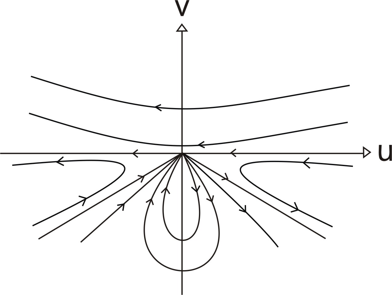 Figure 1
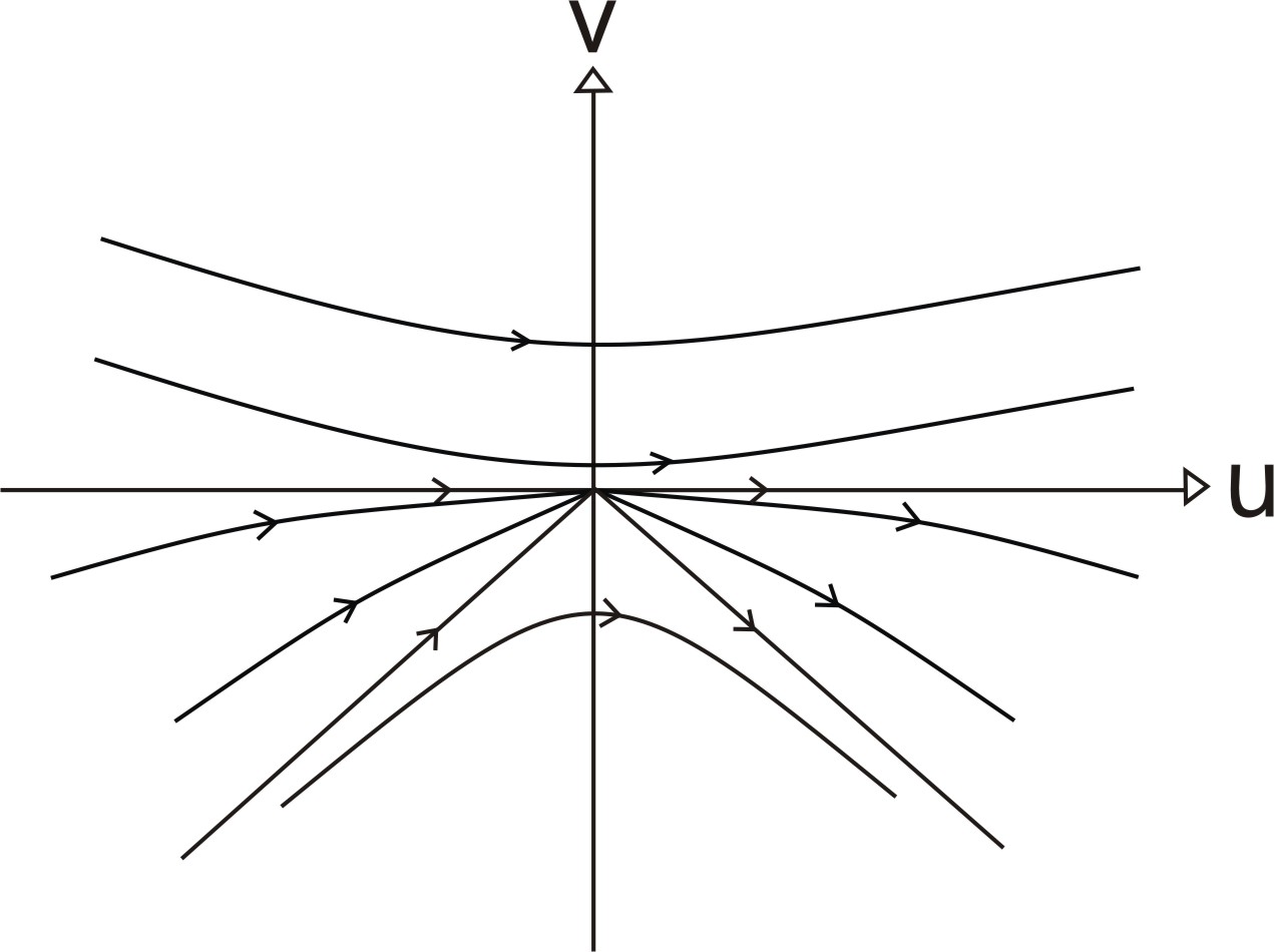 Figure 2
 Figure 3
Peer Reviews
No public reviews on file for this paper yet. If you reviewed it on a platform where reviews are public (OpenReview, ICLR, NeurIPS, ICML), you can paste yours below so the community can read it here.
Videos
No videos yet. Explain this paper in a talk, walkthrough, or lecture? Add one.
Taxonomy
TopicsAdvanced Differential Equations and Dynamical Systems · Quantum chaos and dynamical systems · Mathematical and Theoretical Epidemiology and Ecology Models
Linearizability and critical period bifurcations of
a generalized Riccati system
Valery G. Romanovski1,2,3,4, Wilker Fernandes5, Yilei Tang6,4 and Yun Tian1
1 Department of Mathematics, Shanghai Normal University, Shanghai, 200234, P.R. China
[email protected] (V.G. Romanovski), [email protected] (Y. Tian)
2 Faculty of Electrical Engineering and Computer Science, University of Maribor, Smetanova 17, Maribor, SI-2000 Maribor, Slovenia
3 Faculty of Natural Science and Mathematics, University of Maribor, Koroška c.160, Maribor, SI-2000 Maribor, Slovenia
4 Center for Applied Mathematics and Theoretical Physics, University of Maribor, Krekova 2, Maribor, SI-2000 Maribor, Slovenia
5 Instituto de Ciências Matemáticas e de Computação - USP, Avenida Trabalhador São-carlense, 400, 13566-590, São Carlos, Brazil
[email protected] (W. Fernandes)
6 School of Mathematical Science, Shanghai Jiao Tong University, Dongchuan Road 800, Shanghai, 200240, P.R. China
Corresponding author. [email protected] (Y. Tang)
Abstract.
In this paper we investigate the isochronicity and linearizability problem for a cubic polynomial differential system which can be considered as a generalization of the Riccati system. Conditions for isochronicity and linearizability are found. The global structure of systems of the family with an isochronous center is determined. Furthermore, we find the order of weak center and study the problem of local bifurcation of critical periods in a neighborhood of the center.
Key words and phrases:
Linearizability, isochronicity, global structure, weak center, local bifurcation of critical periods
1. Introduction
A classical problem in the qualitative theory of ordinary differential equations is to characterize the existence of centers and isochronous centers. A singular point of a planar autonomous differential system is called a center if all solutions sufficiently closed to it are periodic, that is, all trajectories in a small neighborhood of the singularity are ovals. If all periodic solutions inside the period annulus of the center have the same period it is said that the center is isochronous.
Poincaré and Lyapunov have shown that the existence of an isochronous center at the origin of a system of the form
[TABLE]
where and are real polynomials without constant and linear terms, is equivalent to the linearizability of the system. This equivalence has made the studies of the isochronicity problem simpler, since the linearizability problem can be extended to the complex field, where the computational methods are more efficient.
The investigation on isochronicity of oscillations started in the 17th century, when Huygens studied the cycloidal pendulum [27]. However, only in the second half of the last century the isochronicity problem began to be intensively studied. In 1964 Loud [34] found the necessary and sufficient conditions for isochronicity of system (1.1) with and being quadratic homegeneous polynomials. Later on, the isochronicity problem was solved for system (1.1) when and are homogeneous polynomials of degree three [40] (see also [29]) and degree five [41]. However in the case of the linear center perturbed by homogeneous polynomials of degree four the problem is still unsolved, although some partial results were obtained [7, 23]. The reason is that linearizability quantities (which are polynomials in the parameters of system (1.1) defined at the beginning of Section 2) have more complicate expressions in the case of homogeneous perturbations of degree four, than in the case of homogeneous perturbations of degree five. There are also many works devoted to the investigation of particular families of some other polynomial systems, see e.g. [1, 6, 9, 14, 35, 43] and references therein. Many works also deal with investigation of isochronicity of Hamiltonian systems, see e.g. [12, 15, 24, 28, 31] and references given there.
The problem of critical period bifurcations is tightly related to the isochronicity problem. In a neighborhood of a center the so-called period function gives the least period of the periodic solution passing through the point with coordinates inside the period annulus of the center. For a center that is not isochronous any value for which is called a critical period. The problem of critical period bifurcations is aimed on estimating of the number of critical periods that can arise near the center under small perturbations. In 1989, Chicone and Jacobs [11] introduced for the first time the theory of local bifurcations of critical periods and solved the problem for the quadratic system. Local bifurcations of critical periods have been investigated for cubic systems with homogeneous nonlinearities [45], the reduced Kukles system [46], the Kolmogorov system [10], the -equivariant systems [8] and some other families (see e.g. [16, 22, 49] and references therein). In [20] a general approach to studying bifurcations of critical periods based on a complexification of the system was described, and some upper bounds on the number of critical periods of several cubic systems were obtained.
In this paper we are interested in the family of Riccati systems. The classic Riccati system is written in the form
[TABLE]
where each is a function with respect to and . System (1.2) becomes a special case of Berouilli system if , and it obviously is a linear differential system if .
The Riccati equation has been invstigated by many authors, see for example [32, 33] and references therein. They are important since they can be used to solve second-order ordinary differential equations and can be applied in studying the third-order Schwarzian differential [37]. It also has many applications in both physics and mathematics. For instance, renormalization group equations for running coupling constants in quantum field theories [5], nonlinear physics [36], Newton’s laws of motion [39], thermodynamics [44] and variational calculus [50].
Recently Llibre and Valls [32, 33] investigated the planar differential system
[TABLE]
which is called the generalized Riccati system, since it becomes the classic Riccati system when . In this paper we study a subfamily of the generalized Riccati system, cubic systems of the form
[TABLE]
where are unknown real functions and are real parameters. Note that system (1.3) is the so-called reduced Kukles system when .
The aims of our study are to obtain conditions on parameters and for the linearizability of system (1.3), to study the global structures of trajectories when the system has an isochronous center, and to investigate the local bifurcations of critical periods at the origin. In Section 2 we present our main result on linearizability, Theorem 2.1, which gives conditions for the linearizability of system (1.3). We also describe an approach for deriving such conditions which is based on making use of modular computations which are performed in the systems of computer algebra Singular [17] and Mathematica [48]. The approach can be applied to investigate many problems involving solving systems of algebraic polynomials. In Section 3 we study the global dynamics of system (1.3) when the origin is an isochronous center. The last section is devoted to the investigation of local bifurcations of critical periods in a neighborhood of the center.
2. Linearizability of system (1.3)
We first briefly remind an approach for studying the isochronicity and linearizability problems for polynomial differential systems of the form
[TABLE]
where and are in .
System (2.1) is linearizable if there is an analytic change of coordinates
[TABLE]
which reduces (2.1) to the canonical linear system , .
Obstacles for existence of a transformation (2.2) are some polynomials in parameters of system (2.1) called the linearizability quantities and denoted by ().
Differentiating with respect to both sides of each equation of (2.2) we obtain
[TABLE]
Substituting in the above equations the expressions from (2.2) and (2.1), one computes the linearizability quantities step-by-step (see e.g. [21] for more details).
From (2.3) it is easy to see that the linearizability quantities are polynomials in parameters of system (2.1). We denote by the -tuple ( is the number of parameters in system (2.1)) of parameters of (2.1), so , and by and the rings of polynomials in with real and complex coefficients, respectively.
Thus, the simultaneous vanishing of all linearizability quantities provides conditions which characterize when a system of the form (2.1) is linearizable. The ideal defined by the linearizability quantities, , is called the linearizability ideal and its affine variety, is called the linearizability variety.
In order to find a linearizing change of coordinates explicitly one can look for Darboux linearization. To construct a Darboux linearization for system (2.1) it is convenient to complexify the system using the substitution
[TABLE]
Then, after a time rescaling by we obtain from (2.1) a system of the form
[TABLE]
System (2.1) is linearizable if and only if system (2.5) is linearizable.
A Darboux factor of system (2.5) is a polynomial satisfying
[TABLE]
where polynomial is called the cofactor of . A Darboux linearization of system (2.5) is an analytic change of coordinates , , such that
[TABLE]
which linearizes (2.5), where , , and and have neither constant terms nor linear terms.
It is easy to see that system (2.5) is Darboux linearizable if there exist Darboux factors with corresponding cofactors , and Darboux factors with corresponding cofactors with the following properties:
- (i)
; 2. (ii)
; and 3. (iii)
there are constants such that
[TABLE]
The Darboux linearization is then given by the transformations
[TABLE]
The readers can consult [13, 35, 43] for more details.
Before passing to the results of our paper we remind some fact about solutions of systems of nonlinear polynomial equations which we will need for our study.
Denote by the ring of polynomials with coefficients in a field and consider a system of polynomials of :
[TABLE]
We recall that the ideal in generated by polynomials , denoted by , is the set of all polynomials of expressed in the form , where are polynomials of . The variety of the ideal in , denoted by , is the zero set of all polynomials of ,
[TABLE]
The situation when the variety of a polynomial ideal consists of a finite number of points arises very rarely. In a generic case, the variety consists of infinitely many points, so generally speaking,“to solve” system (2) means to find a decomposition of the variety of the ideal into irreducible components. More precisely, an affine variety is irreducible if, whenever for affine varieties and , then either or . Let be an ideal and its variety. Then can be represented as a union of irreducible components, where each is irreducible. The radical of denoted by is the set of all polynomials of such that for some non-negative integer is in . Clearly, and have the same varieties. It is known that can be expressed as an intersection of prime ideals, Prime ideals are called the minimal associate primes of . Let () be the variety of . Since the variety of an intersection of some ideals is equal to the union of the varieties of the ideals, we have that . For example, if , then , that is, the variety of is the union of two irreducible components: the plane and the line . In the computer algebra system Singular [17] one can compute the minimal associate primes of a given polynomial ideal and, thus, the irreducible decomposition of its variety using the routine minAssGTZ.
Proceeding now to the results of our paper we first state the following theorem on the linearizability of system (1.3).
Theorem 2.1**.**
System (1.3) is linearizable at the origin if one of the following conditions holds:
- (1)
, 2. (2)
, 3. (3)
, 4. (4)
.
Proof.
Using the computer algebra system Mathematica and the standard procedure mentioned above for system (1.3) we have computed the first eight pairs of the linearizability quantities . Their expressions are very large, so we only present the first two pairs in the Appendix. The reader can easily compute the other quantities using any available computer algebra system 111 One can download linearizability quantities , , , , and the Singular code to perform the decomposition of the variety from http://teacher.shnu.edu.cn/_upload/article/files/79/14/ f36e87e342b8b0d6977e6debdeb3/3b818cf4-a6f7-4f07-8669-f4b78e48f733.txt..
The next computational step is to compute the irreducible decomposition of the variety .
Performing the computations by the routine minAssGTZ [18] of Singular [17] over the field of characteristic 32452843 we obtain that is equal to the union of the varieties of four ideals. After lifting these four ideals to the ring of polynomials with rational coefficients using the rational reconstruction algorithm of [47] we obtain the ideals
[TABLE]
The varieties of , , and provide conditions , , and of the theorem, respectively.
To check the correctness of the obtained conditions we use the procedure described in [42]. First, we computed the ideal , which defines the union of all four sets given in the statement of the theorem. Then we check that . According to the Radical Membership Test, to verify the inclusion it is sufficient to check that the Groebner bases of all ideals , (where and is a new variable) computed over are . The computations show that this is the case. To check the opposite inclusion, , it is sufficient to check that Groebner bases of the ideals (where the polynomials ’s are the polynomials of a basis of ) computed over are equal to . Unfortunately, we were not able to perform these computations over however we have checked that all the bases are over few fields of finite characteristic. It yields that the list of conditions in Theorem 2.1 is the complete list of linearizability conditions for system (1.3) with high probability [3].
We now prove that under each of conditions – of the theorem the system is linearizable.
In this case . We consider only the case , since when the proof is analogous. After the change of variables (2.4) system (1.3) becomes
[TABLE]
which is a quadratic system. By Theorem 3.1 of [13] and Theorem 4.5.1 of [43] system (2.8) is Darboux linearizable and, therefore, system (1.3) is linearizable if condition holds.
After substitution (2.4) system (1.3) becomes
[TABLE]
It has the Darboux factors
[TABLE]
with the respective cofactors
[TABLE]
It is easy to verify that (2.6) is satisfied with and . Hence the Darboux linearization for system (2.9) is given by the analytic change of coordinates
[TABLE]
Thus, system (2.9) is linearizable and therefore the corresponding system (1.3) is linearizable as well.
In this case after substitution (2.4) the corresponding system (1.3) is changed to
[TABLE]
System (2.10) has the Darboux factors
[TABLE]
which allow to construct the Darboux linearization
[TABLE]
where and .
For this condition it is easy to see that . We consider only the case , since when the proof is analogous. After transformation (2.4) system (1.3) becomes
[TABLE]
System (2.11) has the Darboux factors
[TABLE]
yielding the Darboux linearization
[TABLE]
where and . ∎
3. Global dynamics of system (1.3) having an isochronous center
Global phase portrait of a planar autonomous system is usually plotted on the Poincaré disc, which is obtained using the Poincaré compactification. We remind the procedure briefly, for more details see for instance [2, 19].
Consider the planar vector field
[TABLE]
where and are polynomials of degree . Let , be the equator of and be the Poincaré compactification of on . On there are two symmetric copies of , and once we know the behaviour of near , we know the behaviour of in a neighbourhood of the infinity. The Poincaré compactification has the property that is invariant under the flow of . The projection of the closed northern hemisphere of on under is called the Poincaré disc, and its boundary is .
Because is a differentiable manifold, we consider the six local charts and for computing the expression of where . The diffeomorphisms and for are the inverses of the central projections from the planes tangent at the points , and respectively. We denote by the value of or for any .
The expression for in the local chart is given by
[TABLE]
for is
[TABLE]
and for is
[TABLE]
The expressions for ’s are the same as that for ’s but multiplied by the factor . In these coordinates always denotes the points of . When we study the infinite singular points on the charts , we only need to verify if the origin of these charts are singular points.
It is said that two polynomial vector fields and on are topologically equivalent if there exists a homeomorphism on preserving the infinity carrying orbits of the flow induced by into orbits of the flow induced by , preserving or not the sense of all orbits.
In this section, we study the global structures of system (1.3) in Poincaré discs for the case when it has an isochronous center listed in Theorem 2.1.
Theorem 3.1**.**
The global phase portrait of system (1.3) possessing an isochronous center listed in Theorem 2.1 is topologically equivalent to one of phase portraits in Fig. 1. More precisely, there exists only one equilibrium of system (1.3) in the plane, which is an isochronous center at the origin. The neighborhood of equilibrium at infinity consists of one elliptic sector and three hyperbolic sectors (or two hyperbolic sectors and two parabolic sectors) under conditions and (or under conditions and ); otherwise, the isochronous center is global.
Proof.
From Theorem 2.1 we have that under conditions – system (1.3) is linearizable. Under conditions and real systems (1.3) becomes the linear system and its phase portrait is presented in Figure 1.A.
Under conditions and system (1.3) becomes
[TABLE]
and
[TABLE]
respectively.
Note that if in (3.1) and in (3.2), then both systems are the canonic linear systems and have a global center shown in Figure 1.A. Thus, we consider the cases when and . In both cases by a linear change of coordinates we can reduce systems (3.1) and (3.2) to systems
[TABLE]
and
[TABLE]
respectively.
System (3.3) has only the isochronous center at as a finite singular point. Now we analyze its singular points at infinity. In the local chart system (3.3) becomes
[TABLE]
This system has no real singular points. So the unique possible infinite singular point is the origin of the local chart . In the local chart system (3.3) becomes
[TABLE]
It is clear that is a singular point of (3.5) and the linear part of (3.5) at is the null matrix, i.e, \left(\begin{array}[]{cc}0&0\\ 0&0\end{array}\right). Applying the directional blow-up in the -axis twice we obtain that the behaviour of the orbits close to the origin of is as in Figure 3. Therefore, the global phase portrait of system (3.3) is topologically equivalent to the one in Figure 1.B.
Now we study system (3.4). This system has only the isochronous center at as a finite singular point. For the infinite singular points, in the local chart system (3.4) becomes
[TABLE]
This system has only as a singular point, and the linear part of (3.6) at is the null matrix. Applying the directional blow-up in the -axis twice we obtain that the behaviour of the orbits close to the origin of is as showing in Figure 3.
In the local chart system (3.4) becomes
[TABLE]
As it is mentioned above, we need to study only the origin of this chart, but ) is not a singular point for system (3.7). Thus, the global phase portrait of system (3.4) is topologically equivalent to the portrait in Figure 1.C. ∎
4. Weak center and local bifurcation of critical periods
Let be the string of parameters of real system (2.1) with a center at the origin. Changing the system to the polar coordinates , and eliminating , we obtain
[TABLE]
where and are polynomials of and . The solution of equation (4.1) satisfying the initial condition may be locally represented as a convergent power series in ,
[TABLE]
Substituting (4.2) into (4.1), one can find coefficients by successive integration.
Assuming that is the closed trajectory through , we can compute the period function as
[TABLE]
The period function is even and has the Taylor series expansion
[TABLE]
where and coefficients ’s are polynomials in parameters of system (2.1) (see e.g. [1, 11, 35, 43]).
If and , then the origin of system (2.1) is a weak center of order . If for each , then the origin is an isochronous center. For a center which is not isochronous, a local critical period is any value for which .
By classical results of local critical period bifurcations [11], at most local critical periods can bifurcate from the period function related to a weak center of order . In order to prove that there are perturbations with exactly local critical periods, we remind Theorem 2 of [49] as follows.
Theorem 4.1**.**
Assume that the period constants () of system (2.1) depend on independent parameters . Suppose that there exists such that
[TABLE]
and
[TABLE]
then critical periods bifurcate from the center at the origin of system (2.1) after small appropriate perturbations.
Remark. The proof that critical periods can bifurcate after perturbations of system (2.1) corresponding to parameters is derived using the Implicit Function Theorem, and the proof that the bound is sharp can be derived either using the Mean Values Theorem [26] or Rolle’s Theorem [4]. In practice critical periods can be obtained choosing perturbations such that for some system close to
[TABLE]
and the signs in the sequence alternate (see e.g. [25, 30, 43] for more details).
Because bifurcations of critical periods are bifurcations from centers, to study them for system (1.3) we need to know the center variety of the system. Due to computational difficulties the center variety of system (1.3) has been found only in the case when [51]. So, from now on we assume that in system (1.3) and consider the system
[TABLE]
The centers of system (4.4) are identified in the following theorem.
Theorem 4.2** ([51]).**
System (4.4) has a center at the origin if the 7-tuple of its parameters belongs to the variety of one of the following prime ideals:
- (1)
, 2. (2)
, 3. (3)
, 4. (4)
, 5. (5)
, 6. (6)
, 7. (7)
.
Remark. Like in the proof of our Theorem 2.1 modular computations were used in order to determine centers of system (4.4), so it can happen that the list of centers of the system given in Theorem 4.2 is incomplete. For this reason it stands in the theorem ”if” but not ”if and only if”.
We consider the local bifurcations of critical periods for system (4.4) when all parameters are real. Because in the variety of consists of one point which is the origin , we only need to consider varieties of first six ideals .
Theorem 4.3**.**
*Suppose that the origin of system (4.4) is a weak center of a finite order.
(1) Then the order is at most . More precisely, the order is at most (resp. ) when parameters belong to the variety of the ideal (resp. ).
(2) Moreover, at most (resp. ) critical periods can be bifurcated from the weak center of system (4.4) and there exists a perturbation with exactly (resp. ) critical periods bifurcated from when parameters belong to the variety of the ideal (resp. ).*
Proof.
When the parameter belongs to the variety of the ideal , we found that the first four period coefficients of (4.3) are
[TABLE]
We omit the expression of , since it is long and the number of its terms is .
We compute the decomposition of with minAssGTZ and obtain . That is, the condition yields that , showing that the origin is an isochronous center of system (4.4) in this case by Theorem 2.1.
Solving the equation we get
[TABLE]
Substituting (4.5) in , we obtain
[TABLE]
Thus, when the origin is a weak center of order . When , from we find that
[TABLE]
We now employ the procedure Reduce of computer algebra system Mathematica for the set of equalities and inequalities , and find that this semi-algebraic system is fulfilled if and only if and
[TABLE]
Assuming that , we can calculate one of solutions from above equation, which indicates the existence of solutions of above equation with respect to parameters and in real field. Moreover, computing with Mathematica the rank of the matrix
[TABLE]
we find that it is equal to when , and (4.6) holds. From Theorem 4.1 there exists a perturbation of system (4.4) with exactly critical periods bifurcated from weak center of order when belongs to the variety of .
When the parameter belongs to the variety of the ideal , we have the first period coefficient in (4.3):
[TABLE]
which cannot be equal to zero in the real field, since unless . That is, the center at the origin is of order [math] in this case.
When the parameter lies in the variety of the ideal , we compute the first period coefficient in (4.3):
[TABLE]
finding that unless all parameters vanish. Thus the center is of order [math] in this case.
When the parameter belongs to the variety of the ideal or , we can see that system (4.4) is a reduced Kukles system. The variety of ideal (resp. ) for center conditions corresponds to the center type (resp. or ) in [46]. Applying Theorems 3.3, 3.4 and 3.7 of [46] we obtain that the order at the origin is at most (resp. ), and there exists a perturbation with exactly (or ) critical periods bifurcated from when parameters belong to the variety of the ideal (resp. ).
When the parameter belongs to the variety of the ideal , we found that the first three period coefficients in (4.3) are
[TABLE]
Eliminating from we find
[TABLE]
Letting we obtain from that
[TABLE]
yielding
[TABLE]
Eliminating and by substituting and into , we obtain
[TABLE]
which does not vanish if . Therefore, the order of the weak center is at most , and there exists a perturbation with exactly critical periods bifurcated from when parameters belong to the variety of the ideal by Theorem 4.1, since the rank of the matrix
[TABLE]
is equal to when , and . Notice that when and the center is a weak center of order , and when the center is either the linear isochronous center or the order is [math]. ∎
5. Conclusion
For cubic generalized Riccati system (1.3), we derived conditions on parameters of the system for the linearizability of the origin, see conditions - of Theorem 2.1.
For the study we have used the approach based on the modular calculations of the set of solutions of polynomial systems, which was used for the first time in [41] and described in details in [42]. The approach can be considered as one between precise symbolic computations and numerical computations since it produces a result which is not completely correct, but correct with high probability – in the sense that it is easily verified if the obtained solutions of a given system of polynomials are correct, but it can happen, that some solutions are lost. Recently an efficient algorithm to verify if the list of solutions obtained with the approach is complete was proposed in [38] however it is not yet implemented in freely available computer algebra systems. The approach can be efficiently applied to study various mathematical models where arises the problem of solving polynomial equations.
When the origin is an isochronous center, we found that system (1.3) has at most three topologically equivalent global structures, which are the global center at the origin, the neighborhood of equilibrium at infinity consists of one elliptic sector and three hyperbolic sectors, and the neighborhood of equilibrium at infinity consists of two hyperbolic sectors and two parabolic sectors, as shown in Theorem 3.1. The last result is the investigation of local bifurcations of critical periods in a neighborhood of the center. We proved that the order of weak center at the origin is at most when parameters belong to the center variety and at most critical periods can be bifurcated from the weak center of system (4.4), as shown in Theorem 4.3.
Acknowledgements
The first author acknowledges the financial support from the Slovenian Research Agency (research core funding No. P1-0306). The second author is partially supported by a CAPES grant. The third author has received funding from the European Union’s Horizon 2020 research and innovation programme under the Marie Sklodowska-Curie grant agreement No 655212, and is partially supported by the National Natural Science Foundation of China (No. 11431008) and the RFDP of Higher Education of China grant (No. 20130073110074). The first, second and third authors are also supported by Marie Curie International Research Staff Exchange Scheme Fellowship within the 7th European Community Framework Programme, FP7-PEOPLE-2012-IRSES-316338. The forth author is partially supported by the National Natural Science Foundation of China (No. 11501370). The first author thanks Professor Maoan Han for fruitful discussions on the work.
Appendix
Here are listed the first two pairs of the linearizability quantities of system (1.3).
[TABLE]
The reference list from the paper itself. Each links out to its DOI / PubMed record.
- 1[1] V. V. Amel’kin, N. A. Lukashevich, A. P. Sadovskii, Nonlinear Oscillations in Second Order Systems (Russian), Belarusian State University, Minsk, 1982.
- 2[2] A. A. Andronov, E. A. Leontovitch, I. I. Gordon, A. G. Maier, Qualitative Theory of Second-Order Dynamic Systems , Israel Program for Scientific Translations, John Wiley and Sons, New York, 1973.
- 3[3] E. A. Arnold, Modular algorithms for computing Grobner bases, J. Symbolic Comput. 35 (2003) 403–419.
- 4[4] N. N. Bautin, On the number of limit cycles which appear with the variation of coefficients from an equilibrium position of focus or center type, Mat. Sb. 30 (1952) 181–196; Amer. Math. Soc. Transl. 100 (1954) 181–196.
- 5[5] I. L. Buchbinder, S. D. Odintsov, I. L. Shapiro, Effective Action in Quantum Gravity , p. 282, IOP Publishing Ltd, 1992.
- 6[6] J. Chavarriga, I. A. García, J. Giné, Isochronicity into a family of time-reversible cubic vector fields, Appl. Math. Comput. 121 (2001) 129-145.
- 7[7] J. Chavarriga, J. Giné, I. A. García, Isochronous centers of a linear center perturbed by fourth degree homogeneous polynomial, Bull. Sci. Math. 123 (1999) 77-96.
- 8[8] T. Chen, W. Huang, D. Ren, Weak centers and local critical periods for a 𝐙 2 subscript 𝐙 2 \mathbf{Z}_{2} -equivariant cubic system, Nonlinear Dyn. 78 (2014) 2319–2329.