Nonuniform currents and spins of relativistic electron vortices in a magnetic field
Koen van Kruining, Armen G. Hayrapetyan, J\"org B. G\"otte

TL;DR
This paper provides a relativistic quantum mechanical analysis of electron vortex beams in magnetic fields, revealing complex current structures, conditions for zero spin-orbit mixing, and nonuniform spin polarization.
Contribution
It introduces a detailed relativistic model of electron vortex beams, highlighting the conditions for zero spin-orbit mixing and analyzing spin polarization in magnetic fields.
Findings
Electron vortex beams exhibit complex azimuthal current structures.
Existence of vortex beams with zero spin-orbit mixing in relativistic regimes.
Spin polarization varies across the beam, making spin and orbital degrees inseparable.
Abstract
We present a relativistic description of electron vortex beams in a homogeneous magnetic field. Including spin from the beginning reveals that spin-polarized electron vortex beams have a complicated azimuthal current structure, containing small rings of counterrotating current between rings of stronger corotating current. Contrary to many other problems in relativistic quantum mechanics, there exists a set of vortex beams with exactly zero spin-orbit mixing in the highly relativistic and nonparaxial regime. The well defined phase structure of these beams is analogous to simpler scalar vortex beams, owing to the protection by the Zeeman effect. For states that do show spin-orbit mixing, the spin polarization across the beam is nonuniform rendering the spin and orbital degrees of freedom inherently inseparable.
Click any figure to enlarge with its caption.
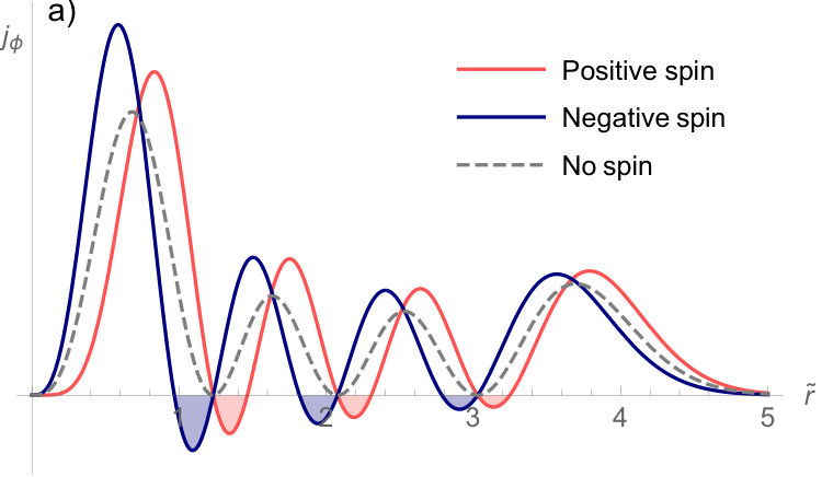 Figure 2
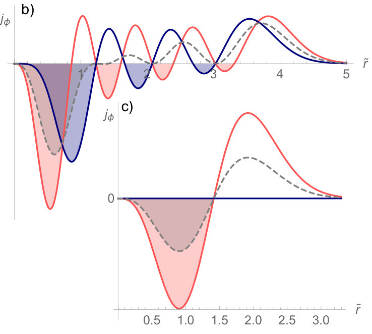 Figure 2
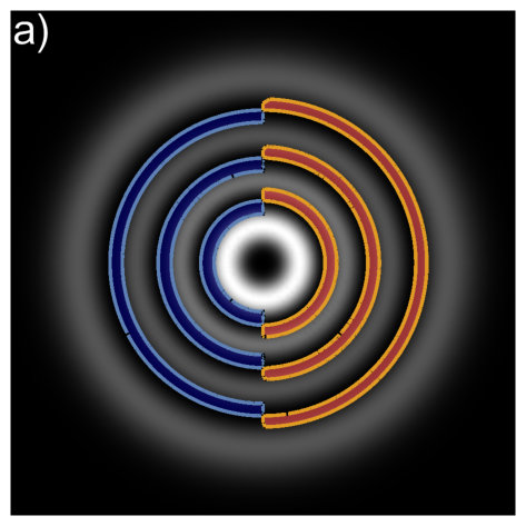 Figure 3
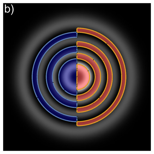 Figure 3
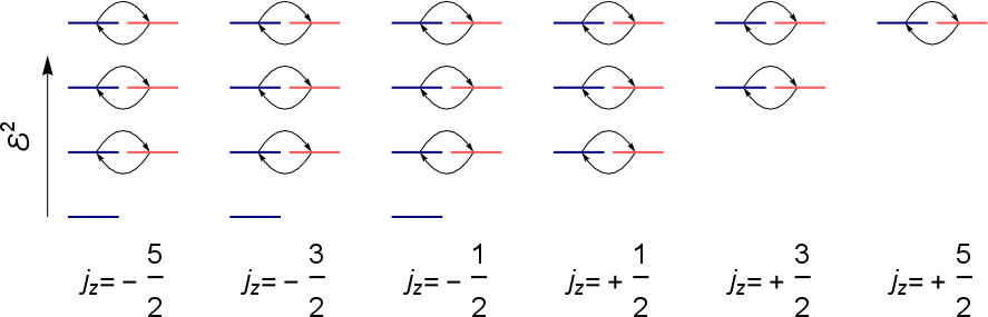 Figure 5
Peer Reviews
No public reviews on file for this paper yet. If you reviewed it on a platform where reviews are public (OpenReview, ICLR, NeurIPS, ICML), you can paste yours below so the community can read it here.
Videos
No videos yet. Explain this paper in a talk, walkthrough, or lecture? Add one.
Nonuniform currents and spins of relativistic electron vortices in a magnetic field.
Koen van Kruining
Armen G. Hayrapetyan
Max-Planck-Institut für Physik komplexer Systeme, 01187 Dresden, Germany
Jörg B. Götte
Nanjing University, Nanjing 210093, China
University of Glasgow, Glasgow G12 8QQ, United Kingdom
Abstract
We present a relativistic description of electron vortex beams in a homogeneous magnetic field. Including spin from the beginning reveals that spin-polarized electron vortex beams have a complicated azimuthal current structure, containing small rings of counterrotating current between rings of stronger corotating current. Contrary to many other problems in relativistic quantum mechanics, there exists a set of vortex beams with exactly zero spin-orbit mixing in the highly relativistic and nonparaxial regime. The well defined phase structure of these beams is analogous to simpler scalar vortex beams, owing to the protection by the Zeeman effect. For states that do show spin-orbit mixing, the spin polarization across the beam is nonuniform rendering the spin and orbital degrees of freedom inherently inseparable.
Introduction— The concept of light beams carrying orbital angular momentum along the propagation axis has been widely utilized in modern optics Allen et al. (1999); Molina-Terriza et al. (2007); Franke-Arnold et al. (2008). Based on analogies of the governing wave equations, vortex beams have also been predicted and generated for electrons Bliokh et al. (2007); *BliokhDennisNori11; *BliokhNori12b; Uchida and Tonomura (2010); Verbeeck et al. (2010); McMorran et al. (2011); Verbeeck et al. (2011); van Boxem et al. (2013); Grillo et al. (2014a); *GGMFKB15; *GrilloKarimiGFDennisBoyd14; Larocque et al. (2016); Thirunavukkarasu et al. (2017) and neutrons Clark et al. (2015), as well as proposed for atoms Hayrapetyan, Armen G. et al. (2013); Lembessis et al. (2014). This promises the ability to probe and manipulate matter on smaller length scales, but also opens up the possibility to consider the interaction of vortex beams with external fields Bliokh et al. (2012); Greenshields et al. (2012); *GreenshieldsFranke-ArnoldStamps15; Karlovets (2012); Hayrapetyan et al. (2014); Guzzinati et al. (2013); *SchattschneiderSS-PLofflerS-TBliokhNori14, other vortex beams Bialynicki-Birula (2004); *Bialynicki-BirulaChmura05; *Bialynicki-BirulaRadozycki06; Ivanov (2011); *IvanovSerbo11; *Ivanov12; *IvanofSSurzhykovFritzsche16 and atoms Matula et al. (2014); *Serboetal15; *ZaytsevSerboShabajev17.
In the simplest description these vortex beams are scalar and obey the paraxial Schrödinger equation. Going beyond the paraxial approximation reveals a linking between the spin and orbital degrees of freedom arising whenever the beam is tightly confined, complicating the vortex structure Barnett (2017); Bialynicki-Birula and Bialynicka-Birula (2017). And whereas light beams as solutions of Maxwell’s equation are naturally relativistic, for particles it is important to distinguish between the nonrelativisitic regime based on Schrödinger’s equation and the relativistic regime covered by the Dirac equation.
Whether or not a nonrelativistic description suffices depends not only on the energy of the electron beam involved, but also on the importance the spin of the particle in the interaction in question, as spin is naturally included in the Dirac equation Dirac (1928); Lifshitz et al. (1991). For electrons traveling through a magnetic field it is of particular importance to take the spin into account, because it interacts strongly with the field.
We analytically solve the Dirac equation for an electron in a homogeneous magnetic field, a problem first considered by Landau Landau and Lifshitz (1991); Lifshitz et al. (1991). The interaction with the magnetic field confines the beam and gives rise to a set of discrete energy levels (Landau levels) Landau and Lifshitz (1991); Bliokh et al. (2012). On top of that the Zeeman effect shifts the energy of the positive and negative spin states relative to each other. The quantized Landau and Zeeman contributions to the energy determine which states undergo spin-orbit mixing with each other and completely forbid spin-orbit mixing for some of them. The inclusion of spin also leads to a (for some states large) redistribution of the azimuthal current within the beam, revealing a pattern of concentric rings of clockwise and counterclockwise rotating current. Our results and conclusions are not only applicable to electrons propagating in beams, but also for electrons confined in Penning traps.
Throughout this letter we set , use the standard representation for the Dirac matrices, slashes to denote contraction with Dirac matrices, the positive z-axis as quantization axis for angular momentum and the metric signature diag( ).
Electron beams in a magnetic field and their spin-orbit structure— A magnetic field can be incorporated in the Dirac equation using the gauge covariant momentum operator , with the vector potential and the electron charge. Choosing the magnetic field in the positive z-direction we take the vector potential , with the magnitude of the magnetic field. Using cylindrical coordinates and first solving the ‘squared’ Dirac equation , we assume a solution of the form , with the total energy, a bispinor and positive. We rescale the radial coordinate as . At a field strength of one Tesla corresponds to 36 nanometer. The rescaled equation for the spin and radial parts becomes
[TABLE]
with , and the Pauli matrices. The interaction energy of the electrons spin magnetic moment is (=Zeeman energy, ). Is the sum of the electrons orbital kinetic energy and the interaction energy of the orbital magnetic moment (Landau energy). The radial differential equation has the well-known solution Landau and Lifshitz (1991); Bliokh et al. (2012)
[TABLE]
with an associated Laguerre polynomial. Here the -sign is the sign of the orbital angular momentum. For negative orbital angular momentum is independent of because the kinetic and magnetic contributions cancel (FIG. 1). These solutions are nondiffracting Laguerre-Gauss beams, with the radial quantum number indicating how many rings surround the central spot or ring. The solutions of the squared Dirac equation describe superpositions of positive and negative energy states. Applying to the wave functions projects out the positive energy part (the full calculation is in the supplementary material). The physical solutions are
[TABLE]
for each of the four combinations of positive and negative spin and orbital angular momentum. Whenever we derive an expression which is different for these four solutions, we put the corresponding expressions in the same order. The second term in the brackets is the spin-orbit mixing term, which appears because orbital angular momentum is not a good quantum number Dirac (1928).
Of particular interest is the last expression (negative spin and orbital angular momentum). Rewriting Riley et al. (2006), one sees that the spin-orbit term is zero for . The lack of spin-orbit mixing for these states stems from all states having a well defined angular momentum and squared energy. The Zeeman effect shifts the squared energy upwards by for the states with positive spin and downwards by the same amount for the states with negative spin. The Landau quantization generates a squared energy ladder with level spacing , twice the Zeeman shift. So the positive spin states are shifted upward one level compared to the negative spin states (FIG. 1) and for the lowest lying states with negative spin there is no positive spin state with equal squared energy they can spin-orbit mix with.
Without the spin-orbit mixing term, the wave function factorizes into a product state of a constant bispinor and a scalar function. Typically, both for light and electrons, such a simple separation in a spin part and a spatial part is not possible, making these negative angular momentum states quite special. This clean separation of spin and orbital angular momentum also makes the ground states perfectly spin polarized, a condition which otherwise has only been achieved with a more complicated combination of magnetic and electric fields Karimi et al. (2012); Nsofini et al. (2016) high loss of beam intensity Schattschneider et al. (2017) or extremely high laser intensities Dellweg and Müller (2017). That they are (for a given ) the lowest energy states suggests that there should be a way to selectively populate these ‘scalar like’ unperturbed nonparaxial vortex states.
Detailed analysis of the current structure— The detailed charge flow within the beam can be computed using the four current . Integrating its zeroth component over the entire transverse plane gives a useful normalization factor. Using , the integrated probability density is evaluated to be resp.
[TABLE]
The last term in the brackets is in each case . Using , the integrated probability density can in each case be written as . The total current in the z-direction through the transverse plane is
[TABLE]
so the electrons have the same speed as particles with mass . For the transverse current components one can transform the Dirac matrices into
[TABLE]
The radial component is always zero and the azimuthal component is
[TABLE]
where we have used the surface element . Rescaling back to gives a current proportional to . These expressions are quite different from the azimuthal currents for scalar vortex beams in a magnetic field Bliokh et al. (2012), because the spin contribution is included in them as well Ohanian (1986). As can be seen in FIG. 2 the inclusion of the spin current reveals complicated patterns of flows and counterflows, which are absent if spin is neglected. These keep their shape even for magnetic field strengths at which there is no appreciable spin-orbit induced change in the beam profile (FIG. 3)
Nonuniform spin— As a consequence of spin-orbit mixing, the spin polarization of an electron becomes nonuniform, similar to the nonuniform spin appearing in structured light Bliokh and Nori (2012b); *BliokhBekshaevNori14; *BekshaevBliokhNori15; Neugebauer et al. (2015); Antognozzi et al. (2016), which is used for direction sensitive optical switching Kien and Hakuta (2008); *KienRauschenbeutel14a; Junge et al. (2013); *Petersen67; *MSASRauschenbeutel14; *PhysRevX.5.041036; Ramos et al. (2014); *PhysRevA.91.042116; *PhysRevA.93.062104; *PhysRevA.93.063830; Söllner et al. (2015). Its existence can be inferred decomposing the probability current in a spin and an orbital part Gordon (1928); Ohanian (1986) and comparing the z-components of the orbital part and the total current, finding that . The difference has to be made up for by a spin current caused by a spin component perpendicular to 111Both Gordon and Ohanian only consider the free case, but because the probability current is gauge invariant, one can see that one must use the gauge covariant momentum operator if fields are present.. Using it can be shown that the radial spin is zero and the azimuthal spin is , where the sign is given by the sign of the total spin in the z-direction. The ground states’ spin polarization is uniform because their spin-orbit mixing is zero. This in contrast to structured light, where the nonuniformity inevitably appears in any finite width beam.
The difference between a uniformly and a nonuniformly spin polarized state is that for a uniformly polarized state one can always choose a direction along which a spin measurement will certainly give the outcome spin up whereas this is impossible for a nonuniformly polarized state, because spin and spatial degrees of freedom are entangled. For our electron beams this entanglement can be shown by taking their density matrices and tracing out everything except the spin. The remaining mixed spin state is for positive spin
[TABLE]
and the same with the spins interchanged for negative spin, showing that one cannot separate the spin and orbital degrees of freedom.
Gauge covariant angular momentum operator— With our choice of gauge, the exact solutions of the Dirac equation are eigenfunctions of the canonical angular momentum operator () with eigenvalues resp. and . The canonical momentum is not gauge covariant but can be made so by the usual minimal substitution, yielding: . This operator does not have any stationary solution of the Dirac equation or the ‘squared’ Dirac equation as its eigenstate, as can be verified by applying it to any (linear combination of degenerate) basis state. Its expectation value can be computed by adding to the canonical angular momentum, the result is (suppl. mat.)
[TABLE]
[TABLE]
If one would neglect the spin-orbit term, one would always get a half-integer expectation value for the gauge covariant angular momentum, although the states, even without spin-orbit term are not eigenstates of . This fortuitous coincidence has been overlooked in the literature until now, to the best of our knowledge. The reason that the expectation value of is not a half integer number is that the orbital contribution changes by two quanta when or is changed by one whereas the spin contribution changes by the usual one quantum upon spin flip. Therefore the main term and the spin orbit term have different expectation values for and one takes the probability weighted average of the both terms. Does have half-integer expectation values. This last quantity determines the z-component of the magnetic moment, , of the electron as can be verified by computing (details in suppl. mat.)
[TABLE]
showing that the gauge covariant operators are the ones determining the magnetic moment.
Apart from not having any stationary eigenfunctions, the gauge covariant angular momentum operators also do not generate a Lie group. These two properties can be proven more generally. Taking the commutator of two of these operators gives (suppl. mat.)
[TABLE]
showing that they violate the closure axiom for Lie algebras if there is any magnetic field present. For the existence of stationary solutions we change notation and write the components of the gauge covariant momenta and ‘boost’ operators as an antisymmetric tensor . The brackets on the indices indicate antisymmetrization, . With this notation, . Now the existence of physical states that are eigenstates of is only possible if the commutator vanishes. This commutator is (suppl. mat.)
[TABLE]
which vanishes only for an extremely restricted class of possible fields. Taking and writing out the field components explicitly, we have
[TABLE]
So the only possible field that would allow for physical eigenstates of , is a constant electric field in the z-direction.
Conclusion— We have shown that in a homogeneous magnetic field there exist electron vortex beams without spin-orbit mixing and thus with a very ‘clean’ vortex core. For these beams, spin-orbit mixing remains absent even for strong magnetic fields and relativistic speeds. Including the effect of spin reveals an internal rearrangement of the azimuthal current which is quite substantial if the orbital angular momentum and magnetic field point in opposite directions. For electron vortex beams the current scales linearly with the beam intensity and the spin rearrangement of the azimuthal current can be magnified by using a strong enough electron beam. If an electron vortex beam is wide enough, a suitable test particle can probe these current rearrangements similar to how a small dielectric particle can probe the local Poynting vector of a light beam He et al. (1995); O’Neil et al. (2002); Neugebauer et al. (2015); Antognozzi et al. (2016).
Acknowledgements— KvK thanks Valentin Walther for the useful discussion helping him clarify the nature of the nonuniform electron spin. This work was supported by the Engineering and Physical Sciences Research Council of the United Kingdom with grants Nos. EP/I012451/1 and EP/M01326X/1 and the the National Key Research and Development Program of China under contract number 2017YFA0303700.
Obtaining the exact solutions of the Dirac equation in a magnetic field
The solutions of te squared Dirac equation in a constant magnetic field (symmetric gauge) are, using the rescaled coordinate and taking positive
[TABLE]
The exact solutions pf the first order Dirac equation can be obtained by applying to the solutions of the squared Dirac equation. Using
[TABLE]
the de derivatives with respect to and are easy to compute and give resp. and . For the transverse derivatives, one can use the rescaled coordinates to rewrite them as
[TABLE]
The components and give rise to the spin-orbit mixing terms, whose explicit computation is rather lengthy. The following three identities will be of use
[TABLE]
The form of the spin-orbit term depends on the signs of the spin and orbital angular momentum. For spin and orbital angular momentum positive, one has
[TABLE]
Using the recurrence relations for Laguerre polynomials (prime denotes differentiation with respect to ) and , the Laguerre polynomials in the brackets become simply , thus the overall solution of the first order Dirac equation in this case becomes
[TABLE]
Now for positive orbital angular momentum and negative spin, the spin-orbit term is
[TABLE]
Using the recurrence relation
[TABLE]
to rewrite the derivatives of the Laguerre polynomial, one gets
[TABLE]
With the relation this expression simplifies to and the solution of the first order Dirac equation for positive orbital angular momentum and negative spin becomes
[TABLE]
For negative orbital angular momentum and positive spin, one has
[TABLE]
Using , where the prime denotes differentiation with respect to , one can rewrite the first Laguerre polynomial:
[TABLE]
Using again this expression becomes
[TABLE]
Because of , everything but the first term cancels and the solution for the first order Dirac equation for negative orbital angular momentum and positive spin becomes
[TABLE]
The case of negative orbital angular momentum and spin is simple, one has
[TABLE]
and using again , the overall solution of the first order Dirac equation becomes
[TABLE]
Explicit forms of the radial and azimuthal gamma and spin matrices
[TABLE]
Explicit evaluation of .
The quantity appears in the computation of the gauge covariant angular momentum of the electron vortex states. For the four different combinations of positive and negative orbital angular momentum and spin (order the same as in the main text) can be shown to be resp.
[TABLE]
Substituting turns these integrals to
[TABLE]
For Laguerre polynomials, we have the orthogonality relation . Using this relation and , we obtain the following integral identity
[TABLE]
which can be used to evaluate all the integals and obtain
[TABLE]
By noting that is times resp. , , and and rearranging, one gets
[TABLE]
Dividing by and adding the canonical angular momentum, resp. and , one gets for the gauge covariant angular momentum
[TABLE]
Computation of the magnetic moment
Using the explicit form of the azimuthal Dirac matrix, it is easy to see that only the crossterms between the main and spin-orbit parts contribute to the azimuthal current and these can be computed to be
[TABLE]
Now . Substituting the explicit currents into this integral, using and performing the angular integration yields
[TABLE]
Now one can again use and the orthogonality relation of associated Laguerre polynomials to evaluate these integrals
[TABLE]
Commutator identities for the gauge covariant angular momentum operators
For this section we write the angular omentum operators in antisymmetric tensor form. The gauge covariant angular momentum can be split in a spin and an orbital part like
[TABLE]
Because contains no Dirac matrices, one obviously has , so . Writing out the commutator for the -tensor gives
[TABLE]
One can check that if all four indices are different, this commutator is zero. If two indices are the same one can eliminate the identical Dirac matrices and obtain after some algebra
[TABLE]
For the orbital part, we need the commutation relations of the gauge covariant momentum . It is easy to check that
[TABLE]
To get the commutators for the gauge coveriant orbital angular momenta, we need to add (the vector potentias commute with each other). Using that both terms are the same up to the index swap , and using these terms can be evaluated to be
[TABLE]
Using , and putting things together gives
[TABLE]
Then using , and , one gets
[TABLE]
For the commutator , one can first note that commutes with any operator. Again using , one can compute the commutators of the spin and orbital parts seperately using :
[TABLE]
The reference list from the paper itself. Each links out to its DOI / PubMed record.
- 1Allen et al. (1999) L. Allen, M. J. Padgett, and M. Babiker, Prog. Opt. XXXIX , 291 (1999).
- 2Molina-Terriza et al. (2007) G. Molina-Terriza, J. P. Torres, and L. Torner, Nat. Phys. 3 , 305 (2007) . · doi ↗
- 3Franke-Arnold et al. (2008) S. Franke-Arnold, L. Allen, and M. J. Padgett, Laser & Phot. Rev. 2 , 299 (2008) . · doi ↗
- 4Bliokh et al. (2007) K. Y. Bliokh, Y. P. Bliokh, S. Savel’ev, and F. Nori, Phys. Rev. Lett. 99 , 190404 (2007) . · doi ↗
- 5Bliokh et al. (2011) K. Y. Bliokh, M. R. Dennis, and F. Nori, Phys. Rev Lett 107 , 174802 (2011) . · doi ↗
- 6Bliokh and Nori (2012 a) K. Y. Bliokh and F. Nori, Phys. Rev. A 86 , 033824 (2012 a) . · doi ↗
- 7Uchida and Tonomura (2010) M. Uchida and A. Tonomura, Nature 464 , 737 (2010) . · doi ↗
- 8Verbeeck et al. (2010) J. Verbeeck, H. Tian, and P. Schattschneider, Nature 467 , 301 (2010) . · doi ↗