Detection of low dimensionality and data denoising via set estimation techniques
Catherine Aaron, Alejandro Cholaquidis, Antonio Cuevas

TL;DR
This paper investigates set and manifold estimation from random samples, focusing on identifying lower-dimensional structures and denoising data, with theoretical guarantees and practical illustrations.
Contribution
It introduces methods for determining the dimensionality of sets, estimating lower-dimensional manifolds, and denoising data based on set estimation theories.
Findings
Proposes procedures to identify if a set is full-dimensional or lower-dimensional.
Develops algorithms to estimate lower-dimensional manifolds from noisy data.
Provides theoretical guarantees and simulation results demonstrating effectiveness.
Abstract
This work is closely related to the theories of set estimation and manifold estimation. Our object of interest is a, possibly lower-dimensional, compact set . The general aim is to identify (via stochastic procedures) some qualitative or quantitative features of , of geometric or topological character. The available information is just a random sample of points drawn on . The term "to identify" means here to achieve a correct answer almost surely (a.s.) when the sample size tends to infinity. More specifically the paper aims at giving some partial answers to the following questions: is full dimensional? Is "close to a lower dimensional set" ? If so, can we estimate or some functionals of (in particular, the Minkowski content of )? As an important auxiliary tool in the answers of these…
Click any figure to enlarge with its caption.
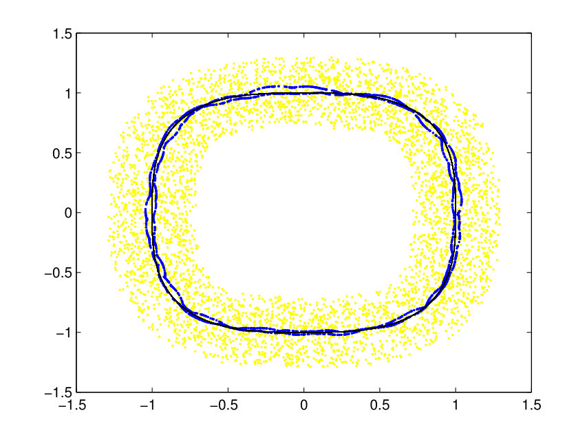 Figure 1
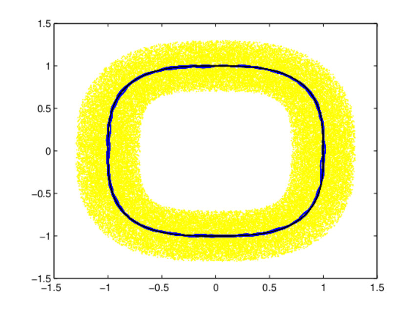 Figure 2
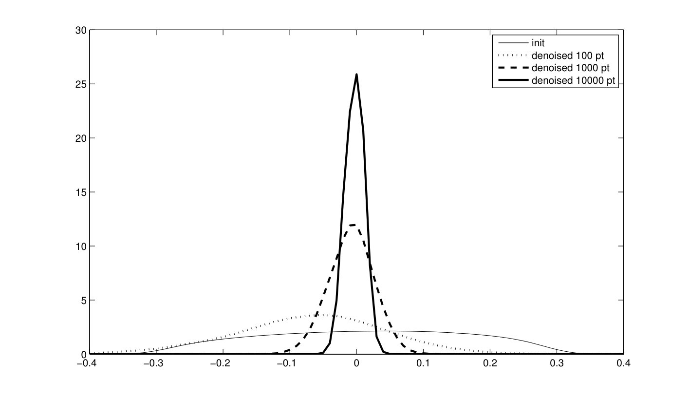 Figure 3
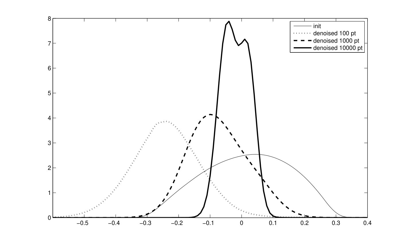 Figure 4
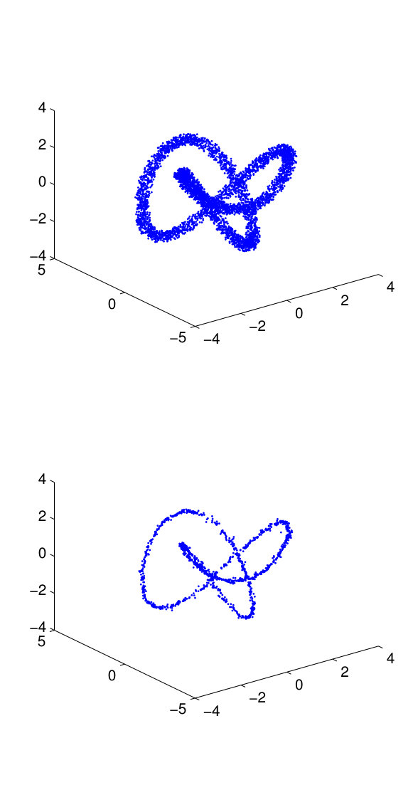 Figure 5
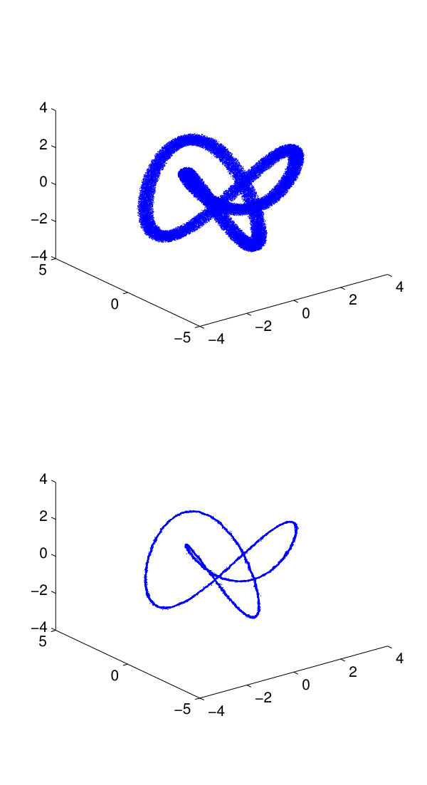 Figure 6
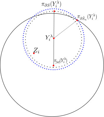 Figure 7
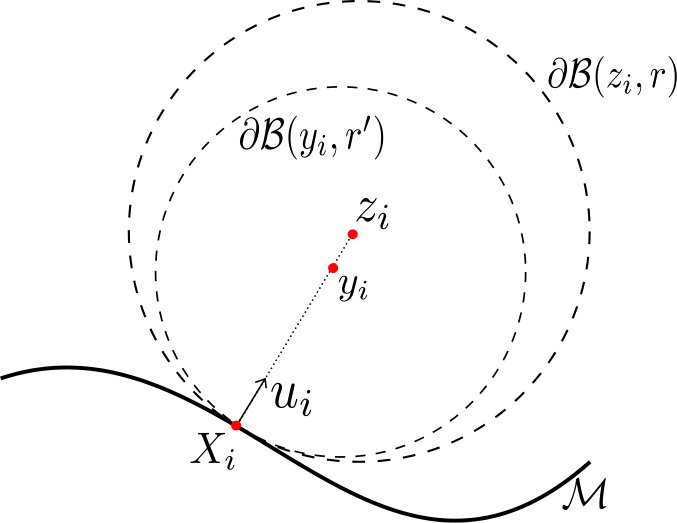 Figure 8
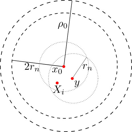 Figure 9
| 0 | |||
|---|---|---|---|
| 0.01 | |||
| 0.05 | |||
| 0.1 | |||
| 0.2 | |||
| 0.3 | |||
| 0.4 | |||
| 0.5 |
Peer Reviews
No public reviews on file for this paper yet. If you reviewed it on a platform where reviews are public (OpenReview, ICLR, NeurIPS, ICML), you can paste yours below so the community can read it here.
Videos
No videos yet. Explain this paper in a talk, walkthrough, or lecture? Add one.
Detection of low dimensionality and data denoising via set estimation techniques
Catherine Aarona, Alejandro Cholaquidisb and Antonio Cuevasc
a Université Blaise-Pascal Clermont II, France
b Centro de Matemática, Universidad de la República, Uruguay
c Departamento de Matemáticas, Universidad Autónoma de Madrid
Abstract
This work is closely related to the theories of set estimation and manifold estimation. Our object of interest is a, possibly lower-dimensional, compact set . The general aim is to identify (via stochastic procedures) some qualitative or quantitative features of , of geometric or topological character. The available information is just a random sample of points drawn on . The term “to identify” means here to achieve a correct answer almost surely (a.s.) when the sample size tends to infinity. More specifically the paper aims at giving some partial answers to the following questions: is full dimensional? Is “close to a lower dimensional set” ? If so, can we estimate or some functionals of (in particular, the Minkowski content of )? As an important auxiliary tool in the answers of these questions, a denoising procedure is proposed in order to partially remove the noise in the original data. The theoretical results are complemented with some simulations and graphical illustrations.
1 Introduction
The general setup and some related literature. The emerging statistical field currently known as *manifold estimation *(or, sometimes, statistics on manifolds, or manifold learning) is the result of the confluence of, at least, three classical theories: (a) the analysis of directional (or circular) data Mardia and Jupp (2000), Bhattacharya and Patrangenaru (2008) where the aims are similar to those of the classical statistics but the data are supposed to be drawn on the sphere or, more generally, on a lower-dimensional manifold; (b) the study of non-linear methods of dimension reduction, Delicado (2001), Hastie and Stuetzle (1989), aiming at recovering a lower-dimensional structure from random points taken around it, and (c) some techniques of stochastic geometry Chazal and Lieutier (2005) and set estimation Cuevas and Fraiman (2010), Cholaquidis et al. (2014), Cuevas et al. (2007) whose purpose is to estimate some relevant quantities of a set (or the set itself) from the information provided by a random sample whose distribution is closely related to the set.
There are also strong connections with the theories of persistent homology and computational topology, Carlsson (2009), Niyogi, Smale and Weinberger (2011), Fasy et al. (2014), Cavanna et al (2015).
In all these studies, from different points of view, the general aim is similar: one wants to get information (very often of geometric or topological type) on a set from a sample of points. To be more specific, let us mention some recent references on these topics, roughly grouped according the subject (the list is largely non-exhaustive):
Manifold recovery from a sample of points, Genovese et al. (2012b); Genovese et al (2012c).
Inference on dimension, Fefferman et al. (2016), Brito et al. (2013).
Estimation of measures (perimeter, surface area, curvatures), Cuevas et al. (2007), Jiménez and Yukich (2011), Berrendero et al. (2014).
Estimation of some other relevant quantities in a manifold, Niyogi, Smale and Weinberger (2008), Chen and Müller (2012).
Dimensionality reduction, Genovese et al. (2012a), Tenebaum et al. (2000).
The problems under study. The contents of the paper. We are interested in getting some information (in particular, regarding dimensionality and Minkowski content) about a compact set . While the set is typically unknown, we are supposed to have a random sample of points whose distribution has a support “close to ”. To be more specific, we consider two different models:
- The noiseless model: the support of is itself; Aamari and Levrard (2015), Amenta et al. (2002), Cholaquidis et al. (2014), Cuevas and Fraiman (1997).
- The parallel (noisy) model: the support of is the parallel set of points within a distance to smaller than , for some , where is a -dimensional set and ; Berrendero et al. (2014). Note that other different models “with noise” are considered in Genovese et al. (2012a), Genovese et al. (2012b) and Genovese et al (2012c).
In Section 3 we first develop, under the noiseless model, an algorithmic procedure to identify, eventually, almost surely (a.s.), whether or not has an empty interior; this is achieved in Theorems 1 and 2 below. A positive answer would essentially entail (under some conditions, see the beginning of Section 3) that has a dimension smaller than that of the ambient space.
Then, assuming the noisy model and ( where denotes the interior of ) Theorems 3 (i) and 4 (i) provide two methods for the estimation of the maximum level of noise , giving also the corresponding convergence rates. If is known in advance, the remaining results in Theorems 3 and 4 allow us also to decide whether or not the “inside set” has an empty interior.
The identification methods are “algorithmic” in the sense that they are based on automatic procedures to perform them with arbitrary precision. This will require to impose some regularity conditions on or . Section 2 includes all the relevant definitions, notations and basic geometric concepts we will need.
In Section 4 we consider again the noisy model where the data are drawn on the -parallel set around a lower dimensional set . We propose a method to “denoise” the sample, which essentially amounts to estimate from sample data drawn around the parallel set around .
In Section 5 we consider the problem of estimating the -dimensional Minkowski measure of under both the noiseless and the noisy model. We assume throughout the section that the dimension (in Hausdorff sense, see below) of the set is known.
Finally, in Section 6 we present some simulations and numerical illustrations.
2 Some geometric background
This section is devoted to make explicit the notations, and basic concepts and definitions (mostly of geometric character) we will need in the rest of the paper.
Some notation. Given a set , we will denote by , , and , the interior, closure, boundary and complement of respectively, with respect to the usual topology of . Let us denote for , where stands for the Euclidean norm. We will also denote . Notice that is equivalent to .
The parallel set of of radius will be denoted as , that is . If is a Borel set, then (sometimes just ) will denote its Lebesgue measure. We will denote by (or , when necessary) the closed ball in , of radius , centred at , and . Given two compact non-empty sets , the *Hausdorff distance *or *Hausdorff-Pompeiu distance *between and is defined by
[TABLE]
Some geometric regularity conditions for sets. The following conditions have been used many times in set estimation topics see, e.g., Niyogi, Smale and Weinberger (2008), Genovese et al. (2012b), Cuevas and Fraiman (2010) and references therein.
Definition 1**.**
Let be a closed set. The set is said to satisfy the outside -rolling condition if for each boundary point there exists some such that . A compact set is said to satisfy the inside -rolling condition if satisfies the outside -rolling condition at all boundary points.
Definition 2**.**
A set is said to be -convex, for , if where
[TABLE]
is the -convex hull of . When is -convex, a natural estimator of from a random sample of points (drawn on a distribution with support ), is .
Following the notation in Federer (1959), let be the set of points with a unique projection on .
Definition 3**.**
For , let reach(S,x)=\sup\{r>0:\mathring{\mathcal{B}}(x,r)\subset{\emph{Unp}}(S)\big{\}}. The reach of is defined by \emph{reach}(S)=\inf\big{\{}\emph{reach}(S,x):x\in S\big{\}}, and is said to be of positive reach if .
The study of sets with positive reach was started by Federer (1959); see Thäle (2008) for a survey. This is now a major topic in different problems of manifold learning or topological data analysis. See, e.g., Adler et al. (2016) for a recent reference.
The conditions established in Definitions 1, 2 and 3 have an obvious mutual affinity. In fact, they are collectively referred to as “rolling properties” in Cuevas, Fraiman and Pateiro-López (2012). However, they are not equivalent: if the reach of is then is -convex, which in turn implies the (outer) -rolling condition. The converse implications are not true in general; see Cuevas, Fraiman and Pateiro-López (2012) for details.
Definition 4**.**
A set is said to be standard with respect to a Borel measure at a point if there exists and such that
[TABLE]
A set is said to be standard if (3) holds for all .
The following results will be useful below. The first one establishes a simple connection between standardness and the inside -rolling condition. The second one (whose proof can be found in Pateiro-López and Rodríguez-Casal (2009)) relates the rolling condition with the reach property.
Proposition 1**.**
Let the support of a Borel measure , whose density with respect to the Lebesgue measure is bounded from below by , if satisfies , then it is standard with respect to , for any and .
Proof.
Let and , if the result is obvious. Let such that . Since there exists such that . Then, for all
[TABLE]
∎
Proposition 2** (Lemma 2.3 in Pateiro-López and Rodríguez-Casal (2009)).**
Let be a non-empty closed set. If satisfies the inside and outside -rolling condition, then .
Some basic definitions on manifolds. The following basic concepts are stated here for the sake of completeness and notational clarity. More complete information on these topics can be found, for example, in the classical textbooks Boothby (1975) and Do Carmo (1992). See also the book Galbis and Maestre (2010) and the summary (Zhang, 2011, chapter 3). Let us start with the classical concept of sub-manifold in (often referred to simply as “manifold”). Denote by the half-space .
Definition 5**.**
A topological sub-manifold of dimension in is a subset of with such that every point in has a neighborhood homeomorphic either to or to .
Those points of having no neighborhood homeomorphic to are called boundary points. If the boundary of (i.e. the set of boundary points of ) is empty we will say that is a (sub-)manifold without boundary.
We will say that a manifold without boundary is a regular -surface, or a differentiable -manifold of class , if there is a family (often called atlas) of pairs (often called parametrizations, coordinate systems or charts) such that the are open sets in and the are functions of class satisfying: (i) , (ii) every is a homeomorphism between and and (iii) for every the differential is injective.
A manifold with boundary is said to be a regular -surface if the set of interior points in is a regular -surface.
A manifold is said to be compact when it is compact as a topological space. As a direct consequence of the definition of compactness, any compact differentiable manifold has a finite atlas. Typically, in most relevant cases the required atlas for a differentiable manifold has, at most, a denumerable set of charts.
An equivalent definition of the notion of manifold (see Do Carmo (1992, Def 2.1, p. 2)) can be stated in terms of parametrizations or coordinate systems of type with . The conditions would be completely similar to the previous ones, except that the are defined in a reverse way to that of Definition 5.
In the simplest case, just one chart is needed. The structures defined in this way are sometimes called planar manifolds.
Some background on geometric measure theory. The important problem of defining lower-dimensional measures (surface measure, perimeter, etc.) has been tackled in different ways. The book by Mattila (1995) is a classical reference. We first recall the so-called Hausdorff measure. It is defined for any separable metric space . Given and , let
[TABLE]
where , . Now, define .
The set function is an outer measure. If we restrict to the measurable sets (according to standard Caratheodory’s definition) we get the -dimensional Hausdorff measure on .
The Hausdorff dimension of a set is defined by
[TABLE]
It can be proved that, when is a -dimensional smooth manifold, .
Another popular notion to define lower-dimensional measures for the case is the Minkowski content. For an integer recall that and define the -dimensional Minkowski content of a set by
[TABLE]
provided that this limit does exist.
In what follows we will often denote , when the value of is understood. The term “content” is used here as a surrogate for “measure”, as the expression (5) does not generally leads to a true (sigma-additive) measure.
A compact set is said to be -rectifiable if there exists a compact set and a Lipschitz function such that . Theorem 3.2.39 in Federer (1969) proves that for a compact -rectifiable set , . More details on the relations between the rectifiability property and the structure of manifold can be found in Federer (1969) Theorem 3.2.29.
3 Checking closeness to lower dimensionality
We consider here the problem of identifying whether or not the set (not necessarily a manifold) has an empty interior.
Note that, if is “regular enough”, is in fact equivalent to . Indeed, in general implies . The converse implication is not always true, even for sets fulfilling the property (see Avila and Lyubich (2007)). However it holds if has positive reach, since in this case (see the comments after Th. 7 and inequality (27) in Ambrosio, Colesanti and Villa (2008)).
Also, clearly, in the case where is a manifold, the fact that has an empty interior amounts to say that its dimension is smaller than that of the ambient space.
3.1 The noiseless model
We first consider the case where the sample information follows the noiseless model explained in the Introduction, that is, the data are assumed to be an sample of points drawn from an unknown distribution with support . When is a lower-dimensional set, this model can be considered as an extension of the classical theory of directional (or spherical) data, in which the sample data are assumed to follow a distribution whose support is the unit sphere in . See, e.g., Mardia and Jupp (2000).
Our main tool here will be the simple *offset *or Devroye-Wise estimator (see Devroye and Wise (1980)) given by
[TABLE]
More specifically, we are especially interested in the “boundary balls” of .
Definition 6**.**
Given let the set estimator (6) based on . We will say that is a boundary ball of if there exists a point such that . The “peeling” of , denoted by , is the union of all non-boundary balls of . In other words, is the result of removing from all the boundary balls.
The following theorem is the main result of this section. It relates, in statistical terms, the emptiness of with .
Theorem 1**.**
Let be a compact non-empty set. Then under the model and notations stated in the two previous paragraphs we have,
(i) if , and fulfills the outside rolling condition for some , then for any set of type (6) with .
(ii) In the case , assume that there exists a ball such that is standard w.r.t to , with constants and (see Definition (4)). Then eventually, a.s., where is a radius sequence such that: for a given .
Proof.
(i) To prove that for all it is enough to prove that for all and for all there exists a point such that
for all . Since is closed and , . The outside rolling ball property implies that for all exists such that . Let us denote , then see Figure 1. Clearly . From and the outside rolling ball property we get that so that, for all , and thus, .
(ii) First we are going to prove that
[TABLE]
Consider only and let , there is a positive constant , such that we can cover with balls of radius centred in . Let us define
[TABLE]
then,
[TABLE]
Notice that for any given ,
[TABLE]
Since , , then using that is standard with the same ,
[TABLE]
Which, according to (8) provides:
[TABLE]
where we have used that . Since , we can choose such that , then, . Finally (7) follows as a direct application of Borel Cantelli Lemma. Observe that (7) implies that eventually a.s. see Figure 2, so there exists such that eventually a.s. Again by (7) we get that, eventually a.s. for all there exists such that and so , which implies that, eventually a.s., is not removed by the peeling process and so eventually, a.s..
∎
Remark 1**.**
Some comments on Theorem 1 are in order, regarding the intuitive meaning of the result itself, the required assumptions and the involved parameters. First note that the outside rolling condition imposed in part (i) is nothing but a geometric smoothness property ruling out the existence of very sharp inward peaks in the boundary of the set. It is close, but not equivalent, to the positive reach condition, as stated in Definition 3. Clearly, the value of the parameter in Theorem 1 is a regularity condition on : the larger , the more regular . In general, if we want to obtain, using statistical methods, some meaningful results on the dimensionality or the interior of , we will need to impose some regularity property. The advantage of the rolling condition is its simple intuitive, almost “visual”, interpretation. See Walther (1999) and Cuevas, Fraiman and Pateiro-López (2012) for further insights on the rolling condition and related properties.
Regarding part (ii): if there must be some ball included in . The standardness assumption imposed in the theorem, only asks that the probability is not “too far from uniformity” on that ball. To be more specific, the probability of the intersection with of any small enough ball centered at a point of must be at most times the volume of . Observe that this mild condition holds, in particular, whenever has a density bounded from below by a positive constant. More insights on the meaning and use of this standardness property can be found, for example, in Cuevas and Fraiman (1997) and Rinaldo and Wasserman (2010).
Finally, about the interpretation of parts (i) and (ii) in the theorem: statement (i) is simple. It just establishes that the property can be identified, with probability one, whatever the simple size using the offset estimator (6) with any radius smaller that the assumed rolling parameter . As for part (ii), let us note that the only relevant parameter is the standardness constant . A conservative choice of would also do the job asymptotically. In this case, the identification of is done asymptotically (eventually, a.s.) by taking the offset estimator with balls of radii depending only on and . The order of such balls appears typically in the convergence rates of many set estimators (see Cuevas and Fraiman (1997), Rodríguez-Casal (2007)) as well as in the theory of multivariate spacings, Janson (1987).
Hence, in summary, the method to identify whether or not is completely “algorithmic” and works, under some regularity conditions on , with probability one. While the situation is easy to identify, the identification of only works asymptotically.
The manifold case. If is assumed to be a manifold, then, under some mild additional assumptions, the identification of low dimensionality can be done in a completely automatic (data-driven) way, with no resort to extra parameters. In other words, the radius of the balls in the auxiliary Devroye-Wise estimator can be chosen as a function of the data in such a way that it is (asymptotically) small enough to identify the situation and large enough to eventually detect , when this is the case.
Theorem 2**.**
Let be a -dimensional compact manifold in . Suppose that the sample points are drawn from a probability measure with support which has a density , with respect the -dimensional Hausdorff measure on , continuous on such that . Let us define, for any , . Then,
if and is a manifold then eventually, a.s..
if and is a manifold without boundary, then eventually, a.s.
Proof.
We will use Theorem 1 (ii). In order to do that, we will prove first that the set is standard. As then is a a compact -manifold. Then we can use the following result, due to Walther (1999).
Theorem (Walther, 1999, Th.1).- Let be a compact path-connected set with and let . Then, the following conditions are equivalent
- 1
A ball of radius rolls freely inside and inside for all .
- 2
is a -dimensional submanifold in with the outward pointing unit normal vector at satisfying the Lipschitz condition
[TABLE]
In fact, the author points out that the result is also valid if the condition of path-connected is dropped and we only assume that every path connected component of has non-empty interior. Hence, note that this result can be applied in our case for since the assumption on the compact hypersurface implies the Lipschitz condition for the outward normal vector and the assumption for every path-connected component of is guaranteed from the fact that every point in has a neighborhood homeomorphic to an open set in . Thus, we may use the result 2 1 in the above theorem to conclude that fulfills both the inside and outside rolling ball property for a small enough radius . Then by Proposition 2 . So, by Proposition 1, satisfies the standardness condition established in Definition 4 with , and . Now, in order to prove that fulfils all the conditions in Theorem 1 (ii) observe that in the full-dimensional case the intrinsic volume in coincides with the restricted Lebesgue measure; see (Taylor, 2006, Prop. 12.6). As a consequence, is equal to the density of w.r.t. the Lebesgue measure restricted to . Let us denote . Note that is in fact the “connectivity statistic”, that is the minimum value of such that is a connected set. Then, as is continuous and bounded below from zero on the compact set with smooth boundary we are in the assumptions of Theorem 1.1 in Penrose (1999) so that, using this result we can conclude that, with probability one, we have,
[TABLE]
Then for large enough,
[TABLE]
now if we denote , it fulfills that , so we are in the hypotheses of Theorem 1 (ii) and then we can conclude eventually, with probability 1.
Notice that we can use Theorem 1 (ii) indeed, as is a compact manifold of by (Thäle, 2008, Prop. 14) it has a positive reach and, thus, it satisfies the outside rolling ball condition (for some radius ). Then it remains to be proved that for large enough. Let us endow with the standard Riemannian structure, where a local metric is defined on every tangent space just by restricting on it the standard inner product on . Under smoothness assumptions, the Riemannian measure induced by such a metric on the manifold agrees with the -dimensional Hausdorff measure on (this is just a particular case of the Area Formula; see (Federer, 1969, 3.2.46)). So we may use Theorem 5.1 in Penrose (1999). As a consequence of that result
[TABLE]
where denotes the geodesic distance on associated with the Riemannian structure. Now, since the Euclidean distance is smaller than the geodesic distance, we have for all , and and finally . Finally from (9) we have , which concludes the proof.
∎
3.2 The case of noisy data: the “parallel” model
The following two theorems are meaningful in at least two ways. On the one hand, if we know the amount of noise ( in the notation introduced before), these results can be used to detect whether or not the support of the original sample is full dimensional (see (11) and (15)).
On the other hand, in the lower dimensional setting, they give an easy-to-implement way to estimate (see (10) and (14)).
Observe that when , then . If denotes a consistent estimator of , a natural plug-in estimator for is .
In Theorem 3 is constructed in terms of the set of the centers of the boundary balls, while in Theorem 4 we use the boundary of the -convex hull. The second theorem is stronger than the first one in several aspects: the parameter choice is easier and the convergence rate is better (and does not depend on the parameter). The price to pay is computational since the corresponding statistic is much more difficult to implement; see Section 6.
Theorem 3**.**
Let be a compact set such that . Let be a constant with and let be an iid sample of a distribution with support , absolutely continuous with respect to the Lebesgue measure, whose density is bounded from below by . Let , with , and let us denote where .
- i)
if then, with probability one,
[TABLE]
- ii)
if then there exists such that, with probability one
[TABLE]
Proof.
Observe, that, since , . Then, the proposed estimator is quite natural: roughly speaking, we may consider that the set of centres of the boundary balls is an estimator of the boundary of so that the maximum distance from the sample points to these centres is a natural estimator of the parameter that measures the “thickness” of . We will now use Corollary 4.9 in Federer (1959); this result establishes that for , the -parallel set of a non-empty closed set fulfills . Also, . Then, in our case, for , this result yields and . By Proposition 1 and 2 in Cuevas, Fraiman and Pateiro-López (2012) fulfils the inner and outer rolling condition.
Another consequence of the positive reach of is that it has a Lebesgue null boundary and thus, with probability one for all , and then, with probability one
[TABLE]
Since , by Proposition 1 is standard with respect to for any constant (see Definition 4).
Now, we will use Theorem 4 and Proposition 1 in Cuevas and Rodriguez-Casal (2004); according to these result, if is partially expandable and it is standard with respect to (both conditions are satisfied in our case) we have for large enough , with probability one,
[TABLE]
for a choice of as that indicated in the above statement of the theorem.
For all let us consider a point such that and where is a normal vector to at that points outside ( can be defined according to Definition 4.4 and Theorem 4.8 (12) in Federer (1959)). Notice that the metric projection of on is thus so, according to (12), with probability one . The point belongs to so, by (13), with probability one for large enough . We thus conclude , with probability one, for large enough. Let then consider , as there exists such that and, as , thus . To summarize we just have proved that: for all there exits such that thus for all : . To conclude (with probability one for large enough).
The reverse inequality is easier to prove, let us consider such that , notice that, by (13) (with probability one for large enough) there exists such that . By triangular inequality and by (13) we also have thus . Then we have proved . This concludes the proof of (10).
Observe that to prove we proved that . Then, with probability one, for large enough, , where .
∎
Theorem 4**.**
Let be a compact set such that . Suppose that the sample has a distribution with support for some with a density bounded from below by a constant . Let us denote where denotes the -convex hull of the sample, as defined in (2) for .
- i)
If and for some has a finite, strictly positive -dimensional Minkowski content, then, with probability one,
[TABLE]
- ii)
if , then there exists such that, with probability one
[TABLE]
Proof.
Again, as shown in the proof of Theorem 3, ; also . We now use Proposition 1 in Cuevas, Fraiman and Pateiro-López (2012); this result establishes that implies that is -convex. According to this result we may conclude that and are both -convex for . Note, in addition, that by construction of we have that for every path-connected component . So, we can use Theorem 3 in Rodríguez-Casal (2007) (which establishes the rates of convergence in the estimation of an -convex set using the -convex hull of the sample) to conclude
[TABLE]
Let us now prove that, with probability one, for large enough,
[TABLE]
Proceeding by contradiction, let x_{n}\in B\big{(}\mathcal{M},R_{1}-d_{H}(\partial C_{r}(\mathcal{Y}_{n}),\partial S)\big{)} such that , let be the projection of onto . It is easy to see that, for large enough, with probability one, then . Observe that, from the definition of parallel set,
[TABLE]
then, there exists , being the open segment joining and , but then by (18), which is a contradiction; this concludes the proof of (17).
Now we can prove . Suppose that . Then . Also, as thus
[TABLE]
For every observation let denote its projection on ; by (17) we have so that, from triangular inequality,
. Thus
[TABLE]
We now analyze the order of the last term in (20). From the assumption of finiteness of the Minkowski content of , given a constant there exists a constant such that for large enough,
[TABLE]
Thus,
[TABLE]
If we take we obtain, from Borel-Cantelli lemma,
[TABLE]
Finally, (14) is a direct consequence of (16), (19), (20) and (21).
The proof of is obtained as in Theorem 3 part . ∎
Remark 2**.**
The assumption imposed on in part (i) can be seen as an statement of -dimensionality. For example if we assume that is rectifiable then, from Theorem 3.2.39 in Federer (1969), the -dimensional Hausdorff measure of , coincides with the corresponding Minkowski content. Hence and, according to expression (4), this entails .
3.3 An index of closeness to lower dimensionality
According to Theorem 3 in the case , the value (where ) can be seen as an index of departure from low-dimensionality. Observe that if we get , a.s. and if has empty interior, a.s.
4 A method to partially denoise the sample data
There are several situations in which we may speak of “noise in the data”: we could first mention the “outlier model” in which the noise is given by a certain amount of outlying observations, far away from the central core of the data. Also, we might have a situation in which every observation is perturbed with a small amount of noise. We will present in this section a denoising proposal, dealing with the latter case and related to the models considered in the previous sections. Before presenting this proposal we will let us briefly comment some references that, from different points of view, deal with the problem of noisy samples in geometric/statistical contexts.
Sometimes the term “denoise” is replaced with “declutter” in the literature on stochastic geometry. A general “declutter algorithm”, depending on a single parameter has bee recently proposed in Buchet et al. (2015). This paper includes also a short interesting overview of the literature on the topic. In particular, the authors mention two main general declutter methodologies, namely procedures based on deconvolution (where the distribution generating the noise appears convolved with the “true” underlying model), see Caillerie et al. (2013), and those based on thresholding, Ozertem and Erdogmus (2011), where the data are “cleaned” using an auxiliary density estimator.
Another interesting approach to the denoising idea, different to that followed in this paper, is given in Chazal et al. (2011). These authors tackle the identification of some geometric or topological features from samples that could include outliers. Again, they use the -offsets (that is the -parallel sets of the sample data and the target set ) as a fundamental tool. Such -offsets are represented in terms of sublevel sets of appropriate functions, defined as a short of distance between a point and a set. The main contribution in the mentioned paper is to robustify (against outliers) such distance functions, and the corresponding sublevel sets, by replacing them with a new function that can be seen as a distance between a point and a probability distribution. A recent related approach, based on the use of kernel density estimates, can be found in Phillips et al (2015).
The denoising idea is also alike to that of identifying (from a sample of points on the set ) the “central part” of the set, often called “skeleton” or “medial axis” of . See Cuevas et al. (2014) and references therein. In fact, the possible idea of defining a denoising procedure in terms of distance to the medial axis, could be seen as a sort of “dual” version of the method proposed in the present paper, based on the distance to the estimated boundary.
Closely related ideas, ultimately relying on the notion of medial axis, are considered in Dey et al. (2015), where a method for “sparsification” of a sample is proposed. The aim is also (as in the denoising case) to retain a subset of the original sample, which is assumed to be drawn on a manifold. In authors’ words: “We sparsify the data so that the resulting set is locally uniform and is still good for homology inference”. The proposed method is based on the “lean feature size” distance, which is intermediate between the well-know “local feature size” (defined in terms of the medial axis) and the “weak local feature size”.
4.1 The algorithm
Let be a compact set with . Let be an iid sample of a random variable , with absolutely continuous distribution whose support is the parallel set for some . We now propose an algorithm to get from , a “partially de-noised” sample of points that allow us to estimate the target set , as established in Theorem 5.
The procedure works as follows:
Take suitable auxiliary estimators for and . Let be an estimator of (based on ) such that eventually a.s., for some . Let be an estimator of such that eventually a.s. for some . 2. 2.
Select a -subsample far from the estimated boundary of . Take and define where if and only if . 3. 3.
The projection + translation stage. For every , we define as follows,
[TABLE]
where denotes the metric projection of on .
4.2 Asymptotics
The following result shows that the above de-noising procedure allows us to asymptotically recover the “inner set” .
Theorem 5**.**
Let be a compact set with . Let be an iid sample of , with support for some , and distribution , absolutely continuous with respect to the Lebesgue measure, whose density , is bounded from below by . Let and be, respectively, the convergence rates in the estimation of , as defined in the algorithm of Sunsection 4.1. Then, there exists such that, with probability one, for large enough,
[TABLE]
where with and denotes the denoised sample defined in the algorithm.
Proof.
First let us prove that eventually a.s.. To do that, we will use Theorem 4 in Cuevas and Rodriguez-Casal (2004) as it was done in Theorem 3. By Corollary 4.9 in Federer (1959), and then by Proposition 1, is standard. Again by Corollary 4.9 in Federer (1959) , which entails, by Proposition 2 that fulfils the outside rolling condition. Using Theorem 4 and Proposition 1 in Cuevas and Rodriguez-Casal (2004) we conclude that, eventually a.s..
Let us fix .
Let us denote and , let us introduce two estimators and . With this notation . Recall that since we have (by Corollary 4.9 in Federer (1959)) that ,
For all there exists a point with so that, by triangular inequality: that is,
[TABLE]
Now let us prove that
[TABLE]
Suppose by contradiction that , since there exists such that , but then . That concludes the proof of (24).
[TABLE]
In the same way it can be proved that
[TABLE]
Let us prove that there exists such that
[TABLE]
First consider the case , which implies that . Notice that, by (25), , finally we get
[TABLE]
Now we consider the case , recall that by (23) and (26) we have.
[TABLE]
In Figure 3 it is represented the case for which takes its largest possible value.
To find an upper bound for such value, let us first note that the points , and are aligned. And the points , and , are aligned. So all of them are in the same plane . Let us now apply a translation T in order to get, . Let us consider in a coordinate system such that .
Let be the coordinates of the point . From (29) we get
[TABLE]
If we multiply (31) by , we get and if we multiply (30) by we get . Then, if we sum this two inequalities we get,
[TABLE]
Notice that , let us denote the coordinates of in , then
[TABLE]
and
[TABLE]
Since the coordinates of are we get that
[TABLE]
Observe that and eventually almost surely. We can bound and , then
[TABLE]
Finally by equations (32), (33) and (34), if (note that this is used in the proof of (32)), there exists such that
[TABLE]
where (see (32)) we are using here. That concludes the proof of (27).
Let us finally prove that eventually, a.s. As indicated at the beginning of the proof, we have eventually a.s., thus for all , there exists such that . For large enough we have . Following the same ideas used to prove (28) we obtain . By triangular inequality we get
[TABLE]
Combining (28), (35) and (36) we obtain,
[TABLE]
∎
Remark 3**.**
Note that, when , the result simplifies since, according to Theorem 3 we can take and, according to Cuevas and Rodriguez-Casal (2004) (Prop. 1 and Th. 4) . Therefore, in this case .
The two following corollaries give the exact convergence rate for the denoising process introduced before, using the centers of the boundary balls (Corollary 1), and the boundary of the -convex hull (Corollary 2), as estimators of the boundary of the support.
Corollary 1**.**
Let be a compact set such that . Let be an iid sample of a distribution with support for some . Assume that is absolutely continuous with respect to the Lebesgue measure and the density , is bounded from below by a constant . Let and .
Given , let be the points obtained after the denoising process using to estimate and as an estimator of where . Then,
[TABLE]
Using the assumption of -convexity for (see Definitions 2 and 3 and the subsequent comments) in the construction of the set estimator, we can replace with (see Theorem 4). Then, at the cost of some additional complexity in the numerical implementation, a faster convergence rate can be obtained. This is made explicit in the following result.
Corollary 2**.**
Let be a compact -dimensional set (in the sense of Theorem 4, i) such that . Let be an iid sample of a distribution with support for some . Assume that is absolutely continuous with respect to the Lebesgue measure and the density , is bounded from below by a constant .
For a given , let be the set of the points obtained after the denoising process, based on the estimator of (for some with ) and the estimator of .
Then,
[TABLE]
5 Estimation of lower-dimensional measures
5.1 Noiseless model
In this section, we go back to the noiseless model, that is, we assume that the sample points are drawn according to a distribution whose support is . The target is to estimate the -dimensional Minkowski content of , as given by
[TABLE]
This is just (alongside with Hausdorff measure, among others) one of the possible ways to measure lower-dimensional sets; see Mattila (1995) for background.
In recent years, the problem of estimating the -dimensional measures of a compact set from a random sample has received some attention in the literature. The simplest situation corresponds to the full-dimensional case . Any estimator of consistent with respect to the distance in measure, that is (in prob. or a.s., where stands for the symmetric difference), will provide a consistent estimator for . In fact, as a consequence of Th. 1 in Devroye and Wise (1980) (recall that is compact here) this will the always the case (in probability) when is the offset estimator (6), provided that is absolutely continuous (on ) with respect to together with and .
Other more specific estimators of can be obtained by imposing some shape assumptions on , such as convexity or -convexity, which are incorporated to the estimator ; see Arias-Castro et al. (2016), Baldin and Reiss (2016), Pardon (2011).
Regarding the estimation of lower-dimensional measures, with , the available literature mostly concerns the problem of estimating , being the boundary of some compact support . The sample model is also a bit different, as it is assumed that we have sample points inside and outside . Here, typically, ; see Cuevas et al. (2007), Cuevas et al. (2013), Jiménez and Yukich (2011).
Again, in the case with , under the extra assumption of -convexity for , the consistency of the plug-in estimator of is proved in Cuevas, Fraiman and Pateiro-López (2012) under the usual inside model (points taken on ). Finally, in Berrendero et al. (2014), assuming an outside model (points drawn in ), estimators of and are proposed, under the condition of polynomial volume for
From the perspective of the above references, our contribution here (Th. 6 below) could be seen as a sort of lower-dimensional extension of the mentioned results of type regarding volume estimation. But, obviously, in this case the Lebesgue measure must be replaced with a lower-dimensional counterpart, such as the Minkowski content (37). We will also need the following lower-dimensional version of the standardness property given in Definition 3.
Definition 7**.**
A Borel probability measure defined on a -dimensional set (considered with the topology induced by ) is said to be standard with respect to the -dimensional Lebesgue measure if there exist and such that, for all ,
[TABLE]
Remark 4**.**
Observe that, by Lemma 5.3 in (Niyogi, Smale and Weinberger (2008)) this condition is fulfilled if has a density bounded from below and is a manifold with positive condition number (also known as positive reach). Standardness of the distribution has also been used in cue04, Chazal et al. (2015), Aamari and Levrard (2015).
Theorem 6**.**
Let be an iid sample drawn according to a distribution on a set . Let us assume that the distribution is standard with respect to the -dimensional Lebesgue measure (see 7) and that there exists the Minkowski content of , given by (37). Let us take such that and , then
- (i)
[TABLE]
- (ii)
If , then
[TABLE]
where \beta_{n}=\mathcal{O}\big{(}\log(n)/n\big{)}^{1/d^{\prime}}.
Proof.
(i) First we will see that, following the same ideas as in Theorem 3 in Cuevas and Rodriguez-Casal (2004) it can be readily proved that, with probability one, for large enough,
[TABLE]
for some large enough constant . In order to see (39), let us consider a minimal covering of , with balls of radius centred in points belonging to . Let us prove that . Indeed, since is a minimal covering it is clear that , and then
[TABLE]
being a positive constant. Since there exists it follows that . Then the proof of (39) follows easily from the standardness of and , so we will omit it.
Now, in order to prove (38), let us first prove that, if we take ,
[TABLE]
To prove this, consider , then there exists such that . Since there exists , . It is enough to prove that . But this follows from the fact that, eventually a.s.,
[TABLE]
Then, from (40)
[TABLE]
Since there exists , the right hand side of (41) goes to zero. To prove that the left hand side of (41) goes to zero, let us observe that, as , and , then
[TABLE]
since and we get
[TABLE]
(ii) The assumption allow us to ensure that has a polynomial volume in the interval . This means that, for , \mu\big{(}B(\mathcal{M},r)\big{)}=P_{d}(r) where is a polynomial of degree at most ; this is a classical result due to Federer (1959, Th. 5.6). Since we assume that the -Minkowski content is finite, this polynomial volume condition entails that the coefficient to the term is . Then,
[TABLE]
for some constant . Now the proof follows from (41) and (42). ∎
Remark 5**.**
In the case of sets with positive reach, part (b) suggests to take since we know by Theorem 1 in Penrose (1999) that r_{n}^{2}=\mathcal{O}\big{(}(\log(n)/n)^{1/d^{\prime}}) that gives the optimal convergence rate.
5.2 Noisy Model
The estimation of the Minkowski content in the noisy model has been tackled in Berrendero et al. (2014), where the random sample is assumed to have uniform distribution in the parallel set . In this section we will see that even if the sample is not uniformly distributed on for some , it is still possible, by applying first the de-noising algorithm introduced in Section 4, to estimate . Following the notation in Section 4, let be an iid sample of a random variable with support , let us denote the de-noised sample defined by (22). The estimator is defined as in (38) but replacing with . Although the subset is not an iid sample (since the random variables are not independent), the consistency is based on the fact that converge in Hausdorff distance to , as we will prove in the following theorem.
Theorem 7**.**
With the hypothesis and notation of Theorem 5, if where with . Then,
[TABLE]
Proof.
The proof is analogous to the one in Theorem 6. Observe that in Theorem 5 we proved that , for some , then . As we did Theorem 6 if we take , then, with probability one,
[TABLE]
then we get
[TABLE]
from where it follows
[TABLE]
Since and we get (43). ∎
6 Computational aspects and simulations
We discuss here some theoretical and practical aspects regarding the implementation of the algorithms. We present also some simulations and numerical examples.
6.1 Identifying the boundary balls
The cornerstone of the practical use of Theorem 1 is the effective identification of the boundary balls. The following proposition provides the basis for such identification, in terms of the Voronoi cells of the sample points. Recall that, given a finite set , the Voronoi cell associated with the point is defined by .
Proposition 3**.**
Let be an sample of points, in , drawn according to a distribution , absolutely continuous with respect to the Lebesgue measure. Then, with probability one, for all and all , if and only if is a boundary ball for the Devroye-Wise estimator (6).
Proof.
Let us take and such that there exists , let us prove that . Observe that since , thus . Reasoning by contradiction suppose that then, with probability one, there exists such that and so that is a contradiction.
Now to prove the converse implication let us assume that is a boundary ball, then there exists such that . Let us prove that (from where it follows that ). Suppose that , then there exists such that and then \mathcal{B}\big{(}z,r-d(z,X_{j})\big{)}\subset\mathring{\hat{S}}_{n}(r). ∎
6.2 An algorithm to detect empty interior in the noiseless case using Theorem 1
In order to use in practice Theorem 1 to detect lower-dimensionality in the noiseless case, we need to fix a sequence under the conditions indicated in Theorem 1 (ii). Note that this requires to assume lower bounds for the “thickness” constant and the standardness constant (see Definition 4) as well as an upper bound for the radius of the outer rolling ball.
Now, according to Theorem 1, and Proposition 3, we will use the following algorithm.
For , let be the vertices of ,
- 2)
Let , since is a convex polyhedron. In the case that is an unbounded cell we put . Define .
- 3)
Decide if and only if .
6.3 On the estimation of the maximum distance to the boundary
Theorems 3 and 4 involve the calculation of quantities such as and , where is a Devroye-Wise estimator of type (6) and is the -convex hull (2) of .
It is somewhat surprising to note that, in spite of the much simpler structure of when compared to , the distance to the boundary can be calculated in a simpler, more accurate way than the analogous quantity for the Devroye-Wise estimator .
Indeed note that is relatively simple to calculate; this is done in Berrendero, Cuevas and Pateiro-López (2012) in the two-dimensional case although can be in fact used in any dimension. Observe first that is included in a finite union of spheres of radius , with centres in . Then . In order to find we need to compute the Delaunay triangulation. Recall that the Delaunay triangulation, , is defined as follows. Let ,
[TABLE]
Observe finally, for any dimension, is a segment or a half line. If is the -dimensional simplex with vertices , the point can be obtained as .
6.4 Experiments
The general aim of these experiments is not to make an extensive, systematic empirical study. We are just trying to show that the methods and algorithm proposed here can be implemented in practice.
Detection of full dimensionality. We consider here a simple illustration of the use of Theorem 1 and the associated algorithm. In each case, we draw 200 samples of sizes 50, 100, 200, 300, 400, 500, 1000, 2000, 5000, 10000 on the -parallel set around the unit sphere, ; that is, the sample data are selected on . The width parameter takes the values . Table 1 provides the minimum sample sizes to “safely decide” the correct answer. This means to correctly decide on, at least 190 out of 200 considered samples, that the support is lower dimensional (in the case ) or that it is full dimensional (cases with ).
We have used the boundary balls procedure (here and in the denoising experiment below for ) with .
The results look quite reasonable: the larger the dimension and the smaller the width parameter , the harder the detection problem.
Denoising. We draw points on in and .
In order to evaluate the effectiveness of the denoising procedure we define the random variable from the denoised data and also from the original data. Note that the “perfect” denoising would correspond to . The Figure 4 shows the kernel estimators of both densities of for the case (left panel) and for (right panel). These estimators for the denoised case are based on values of extracted from samples of sizes 100, 1000, 10000. The density estimators for the initial distribution are based on samples of size 100. Clearly, when the denoised sample of size is based on a very large sample, with , the denoising process is better, as suggested by the fact that the corresponding density estimators are strongly concentrated around 0. The slight asymmetry in the three dimensional case, accounts for the fact that the “external” volume is larger than the “internal” one .
Figures 5 and 6 provide a more visual idea on the result of the denoising algorithm. They correspond, respectively, to the set (where ) and to , where is the so-called Trefoil Knot, a well-known curve with interesting topological and geometric properties.
Minkowski contents estimation. Finally in Table 3 we show, just as a tentative experiment, some results about the Minkowki contents estimation, again in the case of noiseless data () and noisy points (with =0.2) drawn around a sphere for different values for and different dimensions.
For every we estimate the Minkowski contents using a radius (see Theorem 2) when and with a a deterministic radius ( slowly decreasing with the dimension, see Table 2) when . The values of the estimators have been calculated via a Monte Carlo Method based on points uniformly drawn on . For every the experiment has been done times. Table 3 entries provide the average relative error (in percentage) in the estimation of the boundary Minkowski contents . That is, the entries are where , being the correct value of the boundary length in each case, that is , , , for , respectively.
Even if we disregard the intrinsic difficulties associated with the Monte Carlo approximation, the outputs of Table 3 suggest that the denoising-based methodology for the estimation of the Minkowski content from noisy observations, is not accurate for large dimensions. Note however that the problem is intrinsically difficult, as shown by the convergence rates obtained in the noiseless case. Note also that the noise level is quite large, especially for . In any case, the results displayed in Figure 6 suggest a quite reasonable performance of the denoising procedure, for other descriptive or image analysis purposes. Clearly, more research would be needed to reach more definitive conclusions.
Acknowledgements
This research has been partially supported by MATH-AmSud grant 16-MATH-05 SM-HCD-HDD (C. Aaron and A. Cholaquidis) and Spanish grant MTM2016-78751-P (A. Cuevas). We are grateful to Luis Guijarro and Jesús Gonzalo (Dept. Mathematics, UAM, Madrid) for useful conversations and advice.
The reference list from the paper itself. Each links out to its DOI / PubMed record.
- 1Aamari and Levrard (2015) Aamari, E. and Levrard, C. (2015). Stability and minimax optimality of tangential Delaunay complexes for manifold reconstruction. ar Xiv preprint ar Xiv:1512.02857 v 1.
- 2Adler et al. (2016) Adler, R.J., Krishnan, S.R., Taylor, J.E. and Weinberger, S. (2015). Convergence of the reach for a sequence of Gaussian-embedded manifolds. ar Xiv preprint ar Xiv:1503.01733.
- 3Amenta et al. (2002) Amenta, N., Choi, S., Dey, T.K. and Leekha, N. (2002). A simple algorithm for homeomorphic surface reconstruction. Internat. J. Comput. Geom. Appl . 12 , 125–141.
- 4Ambrosio, Colesanti and Villa (2008) Ambrosio, L., Colesanti, A. and Villa, E. (2008). Outer Minkowski content for some classes of closed sets. Math. Ann. 342 , 727–748.
- 5Arias-Castro et al. (2016) Arias-Castro, E., Pateiro-López, B. and Rodríguez-Casal, A. (2016). Minimax estimation of the volume of a set with smooth boundary. ar Xiv preprint ar Xiv:1605.01333 v 1.
- 6Avila and Lyubich (2007) Avila A. and Lybich, M. (2007). Hausdorff dimension and conformal measures of Feigenbaum Julia sets. J. Am. Math. Soc. 21 , 305–363.
- 7Baldin and Reiss (2016) Baldin, N. and M. Reiss (2016). Unbiased estimation of the volume of a convex body. Stochastic Process. Appl. 126 , 3716–3732.
- 8Berrendero, Cuevas and Pateiro-López (2012) Berrendero, J.R., Cuevas, A.. and Pateiro-López, B. (2012). A multivariate uniformity test for the case of unknown support Stat. Comput. 22 , 259–271.