Upper bounds on the minimum coverage probability of model averaged tail area confidence intervals in regression
Paul Kabaila

TL;DR
This paper derives upper bounds on the minimum coverage probability of model averaged tail area (MATA) confidence intervals in complex linear regression models, highlighting limitations of BIC-based weights.
Contribution
It extends previous work by providing an easily computed upper bound for the coverage probability in models with many parameters, demonstrating issues with BIC-based weights.
Findings
Upper bounds indicate potential undercoverage of MATA intervals.
BIC-based weights may lead to inadequate coverage.
Complex models pose challenges for model averaging confidence intervals.
Abstract
Frequentist model averaging has been proposed as a method for incorporating "model uncertainty" into confidence interval construction. Such proposals have been of particular interest in the environmental and ecological statistics communities. A promising method of this type is the model averaged tail area (MATA) confidence interval put forward by Turek and Fletcher, 2012. The performance of this interval depends greatly on the data-based model weights on which it is based. A computationally convenient formula for the coverage probability of this interval is provided by Kabaila, Welsh and Abeysekera, 2016, in the simple scenario of two nested linear regression models. We consider the more complicated scenario that there are many (32,768 in the example considered) linear regression models obtained as follows. For each of a specified set of components of the regression parameter vector, we…
Click any figure to enlarge with its caption.
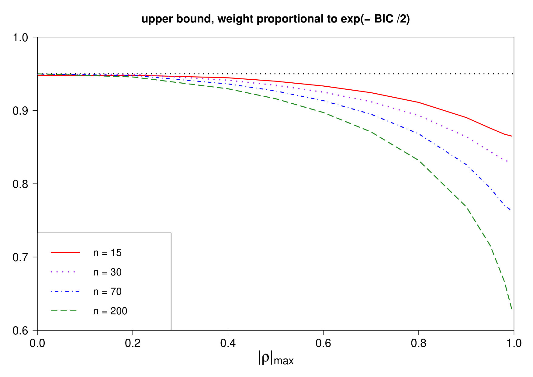 Figure 1
Peer Reviews
No public reviews on file for this paper yet. If you reviewed it on a platform where reviews are public (OpenReview, ICLR, NeurIPS, ICML), you can paste yours below so the community can read it here.
Videos
No videos yet. Explain this paper in a talk, walkthrough, or lecture? Add one.
1
**Upper bounds on the minimum coverage probability of model averaged tail area confidence intervals in regression **
PAUL KABAILA
Department of Mathematics and Statistics
La Trobe University
Key words and phrases: Model averaged confidence intervals; MATA confidence interval; minimum coverage probability.
MSC 2010: Primary 62F25; secondary 62P12
Abstract: Frequentist model averaging has been proposed as a method for incorporating “model uncertainty” into confidence interval construction. Such proposals have been of particular interest in the environmental and ecological statistics communities. A promising method of this type is the model averaged tail area (MATA) confidence interval put forward by Turek & Fletcher, 2012. The performance of this interval depends greatly on the data-based model weights on which it is based. A computationally convenient formula for the coverage probability of this interval is provided by Kabaila, Welsh and Abeysekera, 2016, in the simple scenario of two nested linear regression models. We consider the more complicated scenario that there are many (32,768 in the example considered) linear regression models obtained as follows. For each of a specified set of components of the regression parameter vector, we either set the component to zero or let it vary freely. We provide an easily-computed upper bound on the minimum coverage probability of the MATA confidence interval. This upper bound provides evidence against the use of a model weight based on the Bayesian Information Criterion (BIC).
1. INTRODUCTION
Commonly in applied statistics, there is some uncertainty as to which explanatory variables should be included in the model. Frequentist model averaging has been proposed as a method for properly incorporating this “model uncertainty” into confidence interval construction. Such proposals have been of particular interest in the environmental and ecological statistics communities, see e.g. Fieberg & Johnson (2015, p.712) for a recent review.
The earliest approach to the construction of frequentist model averaged confidence intervals was to first construct a model averaged estimator of the parameter of interest as follows. This estimator is a data-based weighted average of the estimators of this parameter under the various models considered. In this approach, the model averaged confidence interval, with nominal coverage , is centered on this estimator and has width equal to the quantile of the standard normal distribution multiplied by an estimate of the standard deviation of this estimator (Buckland et al., 1997). However, Hjort & Claeskens (2003, Section 4.3) show that the distributional assumption on which this confidence interval is based is completely incorrect in large samples. This problem effectively rules out the use of this confidence interval. Hjort & Claeskens (2003, equation 4.8) then propose a new frequentist model averaged confidence interval that has the desired minimum coverage probability in large samples. However, this interval is essentially the same as the standard confidence interval based on the full model (Kabaila & Leeb, 2006, Remark 5b and Wang & Zou, 2013).
An important conceptual advance was made by Fletcher & Turek (2011) and Turek & Fletcher (2012) who put forward the idea of using data-based weighted averages across the models considered of procedures for constructing confidence intervals. In this way the model averaged confidence interval is constructed in a single step, rather than first constructing a model averaged estimator, which is used as the center of this interval, and then seeking an appropriate formula for the width of this interval. However, some problems have been identified by Kabaila, Welsh & Abeysekera (2016) with the method of Fletcher & Turek (2011). This leaves the model averaged tail area (MATA) confidence interval of Turek & Fletcher (2012) as a promising method, particularly in the normal linear regression context since exactly pivotal quantities for the parameter of interest can be specified for each model under consideration. As Turek & Fletcher (2102) note, their method can also be applied when one has only approximately pivotal quantities for the parameter of interest for each model under consideration. However, the use of such approximately pivotal quantities (which may be obtained by via the parametric bootstrap) is outside the scope of the present paper.
Turek & Fletcher (2012) considered a data-based weight on a model that is proportional to , and , where AIC, and BIC are the Akaike Information Criterion, the Akaike Information Criterion corrected for small samples and the Bayesian Information Criterion, respectively, for the model. The performance of the MATA confidence interval depends greatly on the model weights on which it is based. It is helpful to applied statisticians who wish to use MATA intervals if we can narrow down the choice of data-based model weight by eliminating the worst performing model weights from further consideration.
A computationally convenient formula for the exact coverage probability of the MATA interval is provided by Kabaila, Welsh & Abeysekera (2016) in the simple scenario of two nested normal linear regression models: the full model and a submodel specified by a linear constraint on the regression parameter vector. They consider a parameter of interest that is a specified linear combination of the components of the regression parameter vector for the full model. Kabaila, Welsh & Mainzer (2106) consider the same simple scenario in their evaluation of a MATA interval constructed using data-based weights based on Mallows’ . Of course, it is of interest to also evaluate the MATA interval in the more complicated situations that we average over more than two ( for the real life data considered in Section 5) normal linear regression models.
In the present paper, the family of models that we average over is obtained as follows. For each of a specified set of components of the regression parameter vector, we either set the component to zero or let it vary freely. For the MATA interval, we consider quite general data-based weights on these models. These general weights include, as special cases, the weights considered by Turek & Fletcher (2012) and the weights based on Mallows’ that are considered by Kabaila, Welsh & Mainzer (2016). Using the two new theorems presented in Section 3 of the present paper, we show how the results of Kabaila, Welsh & Abeysekera (2016) can be used to provide a new easily-computed upper bound on the minimum coverage probability of the MATA interval in this situation. This upper bound is analogous to the upper bounds of Kabaila & Leeb (2006) and Kabaila & Giri (2009) on the minimum coverage probability of the post-model-selection confidence interval in the context of the same family of models and is proved using the approach of Kabaila & Giri (2009).
The most important measure (in the form of a single number) of the performance of a confidence interval is its confidence coefficient, defined to be the infimum of the coverage probability of a confidence interval (see e.g. Casella & Berger, 2002, pp.418–419). If the confidence coefficient of a confidence interval is far below its nominal coverage then this confidence interval should not be used. The main application of our new upper bound on the minimum coverage probability of the MATA interval is that it can be used to help eliminate poorly performing model weights from further consideration.
Consider the linear regression model
[TABLE]
where is a random -vector of responses, is a known matrix with linearly independent columns, is an unknown parameter -vector and where is an unknown positive parameter and . Suppose that the quantity of interest is where is a specified non-zero -vector. Our aim is to find a confidence interval for with minimum coverage probability a pre-specified value , based on an observation of .
Henceforth, let denote the family of all subsets of including the empty set, where is a specified integer satisfying . For each , let denote the model for which for all . In other words, the number of models under consideration is . Suppose that the last components of are zeros. In other words, suppose that these models differ from each other only with respect to nuisance parameters, so that the quantity of interest has the same meaning for all of these models. This condition will commonly be satisfied, possibly after some minor reparametrization (see Section 5 for an example). We consider quite general data-based weights on the models , where belongs to the family . We then consider the MATA interval, with nominal coverage , obtained by averaging over the these models using these data-based weights. We denote this confidence interval by .
Our easily-computed (calculated by repeated numerical evaluation of a double integral) upper bound on the minimum coverage probability of the MATA interval is obtained as follows. We first prove the intuitively plausible result Theorem 2 (stated in Section 2) that the wider the class of models over which one averages using specified data-based model weights, the smaller is the minimum coverage probability of the MATA interval, with nominal coverage . Let , denote the least squares estimators of , respectively. Also let corr\big{(}\widehat{\theta},\widehat{\beta}_{j}\big{)} denote the correlation between and , which is a known quantity that is determined by the design matrix and the vector which specifies the parameter of interest . It follows from the results of Kabaila, Welsh & Abeysekera (2016) that the MATA interval, with nominal coverage , obtained by data-based averaging over only the full model and the submodel for which has minimum coverage probability that is the same decreasing function of |\text{corr}\big{(}\widehat{\theta},\widehat{\beta}_{j}\big{)}|, for each . It follows from Theorem 1 that this minimum coverage probability is an upper bound on the minimum coverage probability of the MATA interval , for each . Our upper bound on the minimum coverage probability of the MATA interval is simply the minimum of these upper bounds, which is attained for the value of maximizing |\text{corr}\big{(}\widehat{\theta},\widehat{\beta}_{j}\big{)}|. This upper bound depends on the design matrix and the vector only through the known parameter |\rho|_{\mbox{\footnotesize\rm max}} which we define to be the maximum over of \big{|}\text{corr}\big{(}\widehat{\theta},\widehat{\beta}_{j}\big{)}\big{|}. Since |\rho|_{\mbox{\footnotesize\rm max}} is obtained by this maximization, it may be quite close to 1 in many applications. We have written an R computer program to evaluate this upper bound.
We use this computer program to provide evidence against the use of a data-based weight on the model that is proportional to , where denotes the BIC criterion for this model. Since AIC and BIC are similar criteria for approximately equal to 2, we consider . Figure 1 presents graphs of the upper bound on the minimum coverage probability of the MATA interval , with nominal coverage 0.95, as a function of |\rho|_{\mbox{\footnotesize\rm max}} for and . For each value of considered, this upper bound is found to be a continuous decreasing function of |\rho|_{\mbox{\footnotesize\rm max}} that falls well below when |\rho|_{\mbox{\footnotesize\rm max}} is close to 1. Also, for each value of |\rho|_{\mbox{\footnotesize\rm max}}>0 considered, this upper bound is found to be a decreasing function of . Figures similar to Figure 1 are presented in the Supplementary Material for a wide range of values of and . Figure 1 suggests the following large sample result: under the very weak condition that |\rho|_{\mbox{\footnotesize\rm max}} converges to a positive number as , the minimum coverage probability (i.e the confidence coefficient) of the MATA interval , with weight on model proportional to , converges to 0 as . This suggested result turns out to be correct and is stated in Section 6.
Large sample results can have subtleties in their interpretation. These subtleties are briefly explored at the start of Section 6, before we state the main results of this section. Our conclusion from these results and the Supplementary Material is that the MATA interval with weight on the model proportional to should not be used if |\rho|_{\mbox{\footnotesize\rm max}} is not too far from 1 and is reasonably small, as judged from a figure, such as Figure 1, which is easily computed for any given .
2. THE MATA INTERVAL FOR GENERAL DATA-BASED WEIGHTS
Let denote the least-squares estimator of . Let RSS denote the following residual sum of squares,
[TABLE]
For each , let denote the number of elements in . Also, for , let denote the matrix whose ’th row consists of zeros except for the ’th element which is 1, where is the ’th ordered element of . Thus , for the model (). Let denote the least-squares estimator of subject to this restriction. Note that
[TABLE]
Let denote the residual sum of squares
[TABLE]
and . Also let v(K)=\text{var}\big{(}\boldsymbol{a}^{\top}\widehat{\boldsymbol{\beta}}_{K}\big{)}/\sigma^{2}, where this variance is computed under the model .
We can choose a model from \big{\{}{\cal M}_{K}:K\in{\mathscr{K}}\big{\}} by minimizing the following generalized information criterion
[TABLE]
with respect to , where is a nonnegative number ( for AIC and for BIC) and for . A weight for model () that is proportional to , for either or , was considered by Turek & Fletcher (2012).
We introduce quite general forms of model weights based on the statistics , where
[TABLE]
Some motivation for the use of such weights is provided by the fact that
[TABLE]
is the usual test statistic for testing the null hypothesis that against the alternative hypothesis that . This test statistic has an distribution under this null hypothesis. Obviously, U_{K}/\text{RSS}=V_{K}\big{/}(\text{RSS}/\sigma^{2}), where
[TABLE]
Now, for any given , and are independent random variables, where and has a noncentral chi-squared distribution with degrees of freedom and noncentrality parameter
[TABLE]
see e.g. Graybill (1976, p.127). Thus may be viewed as a data-based measure of the deviation of the model from the true model. This suggests a data-based weight on the model () given by
[TABLE]
Here, the function satisfies the following conditions:
- C1
For each , is a continuous decreasing function of that approaches 0 as . 2. C2
For each , is an increasing function of .
The motivation for the second of these conditions is as follows. According to (4), the weight on model is proportional to , where is a data-based measure of the deviation of the model from the true model and is the number of regression parameters that are set to 0. We want to be an increasing function of since this leads to being a decreasing function of , which is the number of regression parameters in the model . As shown in the appendix, a weight for model () that is proportional to has the form described by (4) above.
The MATA interval for , with nominal coverage and obtained by averaging (using the data-based weights (4)) over the models \big{\{}{\cal M}_{K}:K\in{\mathscr{K}}\big{\}} is obtained as follows. Let
[TABLE]
where is the cdf. The MATA interval I({\mathscr{K}})=\big{[}\widehat{\theta}_{\ell},\widehat{\theta}_{u}\big{]}, is obtained by solving
[TABLE]
for and .
3. TWO IMPORTANT PRELIMINARY RESULTS
Remember the following definitions given in the introduction. Let denote the family of all subsets of (), including the empty set. For each , let denote the model for which for all . Let denote the MATA interval, with nominal coverage , obtained by averaging (using the data-based weights (4)) over the models \big{\{}{\cal M}_{K}:K\in{\mathscr{K}}\big{\}}. Throughout this section we assume that , and are given. Remember, we assume that the last components of are zeros. The following lemma, proved in the appendix, paves the way for Theorems 1 and 2, which are the main results of this section.
Lemma 1. For each given ,
[TABLE]
can be expressed as a function of , and the variables in the set . Also, for , (7) can be expressed as a function of and .
It is intuitively plausible that the wider the class of models over which one averages using specified data-based model weights, the smaller is the minimum coverage probability of the MATA interval, with nominal coverage . Theorem 2 below formalizes this plausible result. Suppose that the integer satisfies . Let denote the family of all subsets of , including the empty set. Obviously, . Let denote the MATA interval, with nominal coverage , obtained by averaging (using the data-based weights (4), but with replaced by ) over the models \big{\{}{\cal M}_{K}:K\in{\mathscr{K}}^{**}\big{\}}. The following theorem is a necessary preliminary to Theorem 2.
Theorem 1.
- (a)
The coverage probability of the MATA interval ,
, is a function of . 2. (b)
The coverage probability of the MATA interval ,
, is a function of .
The proofs of parts (a) and (b) of this theorem are virtually identical and so only part (a) is proved in the appendix.
We will use the following theorem (proved in the appendix) in Section 4 to describe an easily-computed upper bound on the minimum coverage probability of the MATA interval .
Theorem 2. The minimum coverage probability of the MATA interval , with nominal coverage , obtained by averaging (using the data-based weights (4)) over the models \big{\{}{\cal M}_{K}:K\in{\mathscr{K}}\big{\}} is bounded above by the minimum over of
[TABLE]
where denotes the MATA interval, with nominal coverage , obtained by averaging (using the data-based weights (4), but with replaced by ) over the models \big{\{}{\cal M}_{K}:K\in{\mathscr{K}}^{**}\big{\}}.
4. AN EASILY-COMPUTED UPPER BOUND ON THE MINIMUM COVERAGE PROBABILITY OF THE MATA INTERVAL
In this section we present an easily-computed upper bound on the minimum coverage probability of the MATA interval , with nominal coverage , obtained by averaging (using the data-based weights (4)) over the models \big{\{}{\cal M}_{K}:K\in{\mathscr{K}}\big{\}}. Assume, for notational convenience, that \big{|}\text{corr}\big{(}\widehat{\theta},\widehat{\beta}_{j}\big{)}\big{|} is maximized with respect to at . This assumption can always be satisfied using, if necessary, an initial rearrangement of the order of the last columns of the matrix . Theorem 2 implies that this minimum coverage probability is bounded above by the coverage probability of the MATA interval , with nominal coverage , for {\mathscr{K}}^{*}=\big{\{}\varnothing,\{p\}\big{\}} and any given . Theorem 1 of Kabaila, Welsh & Abeysekera (2016) provides a computationally-convenient expression for the latter coverage probability. This expression is easily minimized numerically with respect to to obtain the value of an upper bound on the minimum coverage probability of the MATA interval , with nominal coverage .
To apply Theorem 1 of Kabaila, Welsh & Abeysekera (2016), we introduce the following notation. Let be the -vector , whose first components are zeros. Also let , , and . Observe that is a scaled version of . This scaling is very helpful for the computation of the minimum coverage probability of the MATA interval, as this minimum coverage is achieved at roughly the same value of , for small and moderate sample sizes . Define , which is equal to \boldsymbol{a}^{\top}(\boldsymbol{X}^{\top}\boldsymbol{X})^{-1}\boldsymbol{c}\big{/}(v_{\theta}\,v_{p})^{1/2}. Note that , and are known, whereas is an unknown parameter. Also note that |\widetilde{\rho}|=|\rho|_{\mbox{\footnotesize\rm max}}. Finally, let .
It follows from (4) that the weight w\big{(}{\{p\}},{\mathscr{K}}^{*}\big{)} on the model is given by
[TABLE]
Therefore, the function defined by Kabaila et al. (2016) must satisfy
[TABLE]
so that
[TABLE]
Condition C1 on the function implies that is a decreasing continuous function, such that approaches 0 as . For the particular case that the weight on the model is proportional to , as shown in the appendix, r(x,1)=\exp(d/2)\big{/}(1+x)^{n/2} and consequently
[TABLE]
We now apply the results of Kabaila, Welsh & Abeysekera (2016). The function is defined on page 4 of this paper. As shown on page 6 of this paper, for the scenario considered in the present paper, this function takes the following particular form. For , define to be the solution for in the equation
[TABLE]
where denotes the cdf. An immediate consequence of Theorem 1 of Kabaila, Welsh & Abeysekera (2016) is that the coverage probability of the MATA interval , with nominal coverage , and any given is given by
[TABLE]
where and denote the cdf and pdf, respectively, and denotes the pdf of , where . As noted on page 6 of Kabaila, Welsh & Abeysekera (2016), the conditions required for Theorem 3 of Kabaila, Welsh & Abeysekera (2016) to hold are satisfied. This theorem implies that this coverage probability is an even function of for fixed and an even function of for fixed . The upper bound on the minimum coverage probability of the MATA interval , with nominal coverage , is obtained by setting \widetilde{\rho}=|\rho|_{\mbox{\footnotesize\rm max}} and then minimizing (9) over . The double integral (9) is very easily computed using the methods described in Appendix B of Kabaila, Welsh & Mainzer (2016). An R computer program for the computation of this double integral is available upon request.
5. NUMERICAL ILLUSTRATIONS
In this section, we present some computed values of the upper bound, described in the previous section, on the minimum coverage probability of the MATA interval , with nominal coverage 0.95, obtained using a weight for model () that is proportional to for both (AIC) and (BIC). Consider the real life Air Pollution data described in Section 11.14 of Chatterjee & Hadi (2012). The purpose of collecting this data was to study the dependence of total mortality on climate, socioeconomic and pollution explanatory variables. Let denote the explanatory variable described in Table 11.11 of Chatterjee & Hadi (2012), for . Consider the following linear regression model for this data:
[TABLE]
where the response variable is the total age-adjusted mortality from all causes, are unknown parameters and , for an unknown parameter. In this case, and . Suppose that is the family of all subsets of including the empty set. For each , let denote the model for which for all . In other words, the number of models under consideration is . Suppose that the parameter of interest is for , where is equal to
[TABLE]
Note that is well within the range of the values of in the data. Obviously, and so
[TABLE]
and . In this parametrization of the linear regression model, has the same meaning for all the models , where . In this case, |\rho|_{\mbox{\footnotesize\rm max}}=0.9599 and the upper bound on the minimum coverage probability of the MATA interval , with nominal coverage 0.95, is (a) 0.8900 for (AIC) and (b) 0.7940 for (BIC).
6. LARGE SAMPLE RESULTS FOR THE MATA INTERVAL
The main result of this section provides conditions under which the MATA interval , with weight on model proportional to , has minimum coverage probability (i.e. confidence coefficient) that converges to 0 as . An important advantage of the results presented in Sections 1–5 is that they are exact finite sample results and consequently their interpretation is very straightforward. By contrast, large sample results can have subtleties in their interpretation. It is these subtleties that we briefly explore before stating the main results of this section. We begin by reminding the reader of Hodges’s superefficient estimator and the well-known subtleties in the interpretation of large sample results for this point estimator. We then note that similar subtleties in the interpretation of large sample results also occur in the context of confidence intervals. Finally, we present the main result of this section which concerns the MATA interval.
Hodges’s superefficient estimator is described as follows. Suppose that are independent and identically distributed, where . The usual estimator of is . Of course, nE\big{(}(\overline{X}_{n}-\theta)^{2}\big{)}=1 for all . Hodges’s superefficient estimator is
[TABLE]
where . As shown on p.442 of Lehmann and Casella (1998), \lim_{n\rightarrow\infty}nE\big{(}(T_{n}-\theta)^{2}\big{)}=1 if and \lim_{n\rightarrow\infty}nE\big{(}(T_{n}-\theta)^{2}\big{)}=b^{2} if . Thus, at first sight, it may appear that performs better (in terms of mean squared estimation error) than when the sample size is large. However, as Figure 2.1 on p.443 of Lehmann & Casella (1998) shows, this apparent improvement in performance is misinformative: the supremum over of nE\big{(}(T_{n}-\theta)^{2}\big{)} approaches infinity as . The problem with the analysis of nE\big{(}(T_{n}-\theta)^{2}\big{)} for each fixed as is that this is a limit result that is pointwise in the parameter space . We should, instead, consider nE\big{(}(T_{n}-\theta)^{2}\big{)} across the entire parameter space for each fixed and then let . As pointed out on p.153 of Hajek (1971):
Especially misinformative are those limit results that are not uniform. Then the limit can exhibit some features that are not even approximately true for any finite .
and
Super efficient estimates produced by L.J. Hodges (see LeCam 1953, p.280) have their shocking properties only in the limit. For any finite they behave quite poorly for some parameter values. These values, however, depend on and disappear in the limit.
Kabaila (1995) presents the following confidence interval analogue of Hodges’s superefficient estimator. Suppose that have the same probability distribution as before. Also define and as before. The usual confidence interval for is I_{n}=\big{[}\overline{X}_{n}-n^{-1/2}z_{1-\alpha},\overline{X}_{n}+n^{-1/2}z_{1-\alpha}\big{]}, where the quantile is defined by the requirement that for . Of course, for all and . Let
[TABLE]
where, as before, . Now define the confidence interval J_{n}=\big{[}T_{n}-n^{-1/2}z_{1-\alpha}W_{n}^{1/2},T_{n}+n^{-1/2}z_{1-\alpha}W_{n}^{1/2}\big{]}. It may be shown that for each , . In addition, it may be shown that for and for all . Thus, at first sight it may appear that the confidence interval performs better than the confidence interval when is large. Kabaila (1995) shows that this apparent improvement in performamce is misinformative: the infimum over of approaches 0 as . In other words, the confidence coefficient of approaches 0 as . The problem with the analysis of for each fixed as is that this is a limit result that is pointwise in the parameter space . We should, instead, consider across the entire parameter space for each fixed and then let . This point is also made by Leeb & Pötscher (2005, pp.31–32).
We now present the main results of this section. Consider the linear regression model and parameter of interest described in the introduction. Remember, we assume that the last components of are zeros. Also consider the MATA interval , with nominal coverage and weight on model proportional to , described in Section 4. The large sample framework that we consider is that and are fixed and . Of course, many of the quantities which were defined in Section 4 now depend on . We make this dependence explicit in the notation by using , , , , and to denote , , , , and , respectively. Note that , and are known, whereas is an unknown parameter. The main result of this section requires that the following assumption concerning holds.
Assumption A Suppose that is an increasing sequence of nonnegative numbers that diverges to as . Also suppose that as .
This assumption holds, for example, when , in which case the weight on model is proportional to .
Theorem 3. Consider the linear regression model and parameter of interest described in the introduction. Also consider the MATA interval , with nominal coverage and weight on model proportional to , described in Section 4. Here, {\mathscr{K}}^{*}=\big{\{}\varnothing,\{p\}\big{\}}. Suppose that and are fixed and that exists and is nonsingular. Also suppose that
\boldsymbol{a}^{\top}\boldsymbol{D}^{-1}\boldsymbol{c}\big{/}\big{(}\boldsymbol{a}^{\top}\boldsymbol{D}^{-1}\boldsymbol{a}\,\boldsymbol{c}^{\top}\boldsymbol{D}^{-1}\boldsymbol{c}\big{)}^{1/2}\neq 0. Finally, suppose that Assumption A holds. Then
- (a)
The infimum over of converges to 0, as . 2. (b)
If and () are fixed and then converges in probability to 1 and converges to , as . 3. (c)
If and () are fixed and then converges in probability to 1 and converges to , as .
This result is proved in the appendix. The most important part of this theorem is (a) which implies that the MATA interval, with weight on model proportional to , has confidence coefficient that approaches 0 as . In other words, this MATA interval should not be used when is large. Parts (b) and (c) of this theorem do not provide useful information as they are limits as pointwise in the parameter space.
Another way of looking at Theorem 3 is the following. Consider the asymptotic framework that and () are both fixed. If then and if then diverges to at rate . Sequences that diverge to at a slower rate are not included in this analysis. The proof of part (a) of Theorem 3 presents one such sequence for which the coverage probability of the MATA interval converges to 0. This sequence is “missed” in the asymptotic framework that and are both fixed. In other words, this asymptotic framework does not lead to an accurate appreciation of the confidence coefficient of this MATA interval when is large.
We now turn our attention to the asymptotic framework that is fixed and . The following result is proved in the appendix.
Theorem 4. Consider the linear regression model and parameter of interest described in the introduction. Also consider the MATA interval , with nominal coverage and weight on model proportional to , described in Section 4. T Suppose that is fixed. Also suppose that Assumption A holds. Then, for any given ,
[TABLE]
In other words, converges in probability to 0 as , uniformly in the parameter .
This theorem and its proof suggest that the MATA interval described in this result will be close to the usual confidence interval for based on the full model when is small compared to . An interpretation of this suggested result is that this MATA interval is rather uninteresting when is small compared to . A numerical exploration of the case that is small compared to is presented in the Supplementary Material.
7. CONCLUSION
We have derived an easily-computed new upper bound on the minimum coverage probability (i.e. the confidence coefficient) of the MATA confidence interval in the context of all possible subsets of a given set of explanatory variables in a linear regression model. The main application of this upper bound is that it can be used to help eliminate poorly performing model weights from further consideration. In the Supplementary Material we present graphs similar to those displayed in Figure 1 for a wide range of values of and . These graphs, combined with the large sample results presented in Section 6, show that the MATA confidence interval with weight on a model that is proportional to , where BIC is the Bayesian Information Criterion for this model, should not be used if |\rho|_{\mbox{\footnotesize\rm max}} is not too far from 1 and is not too close to 1.
BIBLIOGRAPHY
Abramowitz, M. & Stegun, I.A. (1965). Handbook of Mathematical Functions with Formulas, Graphs, and Mathematical Tables. Dover, New York.
Buckland, S.T., Burnham, K.P. & Augustin, N.H. (1997). Model selection: an integral part of inference. Biometrics, 53, 603–618.
Casella, G. & Berger, R.L. (2002). Statistical Inference, 2nd edition. Duxbury, Pacific Grove, CA.
Chatterjee, S. & Hadi, A.S. (2012). Regression Analysis by Example, 5th edition. Wiley, Hoboken, NJ.
Fieberg, J. & Johnson, D.H. (2015). MMI: Multimodel inference or models with management implications. Journal of Wildlife Management, 79, 708–718.
Fletcher, D. & Turek, D. (2011). Model-averaged profile likelihood confidence intervals. Journal of Agricultural, Biological and Environmental Statistics, 17, 38–51.
Graybill, F. A. (1976). Theory and Application of the Linear Model. Duxbury, Pacific Grove CA.
Hajek, J. (1971). Limiting properties of likelihoods and inference. In Foundations of Statistical Inference: Proceedings of the Symposium on the Foundatuions of Statistical Inference prepared under the auspices of the Rene Descartes Foundation and held at the Department of Statistics, University of Waterloo, Ontario, Canada, from March 31 to April 9, 1970, V.P. Godambe & D.A. Sprott eds, pp. 142–159. Holt, Reinhart and Winston, Toronto.
Hjort, N.L. & Claeskens, G. (2003). Frequentist model average estimators. Journal of the American Statistical Association, 98, 879–899.
Johnson, N.L., Kotz, S. & Balakrishnan, N. (1995). Continuous Univariate Distributions, Volume 2, 2nd edition. Wiley, New York.
Kabaila, P. (1995). The effect of model selection on confidence regions and prediction regions. Econometric Theory, 11, 537–549.
Kabaila, P. & Leeb, H. (2006). On the large-sample minimal coverage probability of confidence intervals after model selection. Journal of the American Statistical Association, 101, 619–629.
Kabaila, P. & Giri, K. (2009). Upper bounds on the minimum coverage probability of confidence intervals in regression after model selection. Australian & New Zealand Journal of Statistics, 51, 271–287.
Kabaila, P., Welsh, A.H. & Abeysekera, W. (2016). Model-averaged confidence intervals. Scandinavian Journal of Statistics, 43, 35–48.
Kabaila, P., Welsh, A.H. & Mainzer, R. (2016). The performance of model averaged tail area confidence intervals. Communications in Statistics - Theory and Methods, DOI: 10.1080/03610926.2016.1242741
LeCam, L. (1953). On some asymptotic properties of maximum likelihood estimates and related Bayes’ estimates. University of California Press, p.277–328.
Leeb, H. & Pötscher, B.M. (2005). Model selection and inference: facts and fiction. Econometric Theory, 21, 21–59.
Lehmann, E.L. & Casella, G. (1998). Theory of Point Estimation, 2nd edition. Springer, New York.
Turek, D. & Fletcher, D. (2012). Model-averaged Wald confidence intervals. Computational Statistics and Data Analysis, 56, 2809–2815.
Wang, H. & Zou, S.Z.F. (2013). Interval estimation by frequentist model averaging. Communications in Statistics - Theory and Methods, 42, 4342–4356.
APPENDIX
**The function for weight on model proportional to **
Suppose that
[TABLE]
where is given by (2) for each . As noted in Appendix B of Kabaila & Giri (2009), for each ,
[TABLE]
with the convention that for . It follows from this that
[TABLE]
and, for ,
[TABLE]
It follows that is of the form (4) for r(x,y)=\exp(d\,y/2)\big{/}(1+x)^{n/2}, where satisfies conditions C1 and C2.
Proof of Lemma 1
Suppose that is given (). Let denote the -vector obtained from by setting to zero all of the components of with indices belonging to . Since is a subset of , the first components of are . Since we assume that the last components of are zeros, . Thus
[TABLE]
Since ,
[TABLE]
It follows from this and (1) that
[TABLE]
Obviously, \big{(}\widehat{\boldsymbol{\beta}}-\boldsymbol{\beta}_{K}\big{)}\big{/}\sigma=\big{(}\widehat{\boldsymbol{\beta}}-\boldsymbol{\beta}\big{)}\big{/}\sigma+\big{(}\boldsymbol{\beta}-\boldsymbol{\beta}_{K}\big{)}\big{/}\sigma. Hence \boldsymbol{a}^{\top}\big{(}\widehat{\boldsymbol{\beta}}_{K}-\boldsymbol{\beta}_{K}\big{)}\big{/}\sigma can be expressed as a function of \big{(}\widehat{\boldsymbol{\beta}}-\boldsymbol{\beta}\big{)}\big{/}\sigma and the variables in the set .
Now we turn our attention to the denominator of the right-hand side of (11). It follows from (10) that, for each ,
[TABLE]
with the convention that for . Hence, for each ,
[TABLE]
Suppose that . Note that can be expressed as a function of the random variables in the set . Therefore, can be expressed as a function of and the random variables in the set . Hence (11) can be expressed as a function of , and the random variables in the set . Since for all , (11) can be expressed as a function of , and the variables in the set . Also, for , (11) can be expressed as a function of and .
Proof of Theorem 1(a)
It may be shown that, for given , h\big{(}z,\boldsymbol{y};{\mathscr{K}}\big{)} is a continuous decreasing function of . It follows from this that, for any given ,
[TABLE]
Thus the coverage probability of the MATA interval , with nominal coverage , is
[TABLE]
We see from (4) that, for each , is a function of and . It follows from Lemma 1 that the vector of random variables in the set
[TABLE]
can be expressed as a function of , and . Therefore
[TABLE]
can be expressed as a function of , and .
Now and are independent random variables with (\widehat{\boldsymbol{\beta}}-\boldsymbol{\beta})/\sigma\sim N\big{(}\boldsymbol{0},(\boldsymbol{X}^{\top}\boldsymbol{X})^{-1}\big{)} and . Hence (S0.Ex26) is a function of .
Proof of Theorem 2
Suppose that is given. Choose . We will consider . Define to be the family of sets that belong to and include at least one element of the set . Remember, denotes the family of all subsets of , including the empty set. Thus , where and are disjoint sets. Hence
[TABLE]
Now consider to be a given element of . It can be proved that \big{(}\boldsymbol{H}_{K}(\boldsymbol{X}^{\top}\boldsymbol{X})^{-1}\boldsymbol{H}_{K}^{\top}\big{)}^{-1} is a symmetric positive definite matrix. The noncentrality parameter , given by (3), is bounded below by
[TABLE]
where denotes the Euclidean norm. Since and , and so as . Thus
[TABLE]
It follows from condition C1 on the function that
[TABLE]
For each ,
[TABLE]
Therefore, for each , , as . Since
[TABLE]
the first term on the right-hand side of (13) converges in probability to zero as .
For ,
[TABLE]
It follows from (14) that, for each ,
[TABLE]
It follows from (13) that
[TABLE]
By Theorem 1, the coverage probability of the MATA interval , with nominal coverage , is a function of and . Since we suppose that is given, the infimum of this coverage probability over and is less than or equal to
[TABLE]
for every . Also, it follows from (16) that
[TABLE]
approaches
[TABLE]
as . Therefore the infimum of the coverage probability of the MATA interval , with nominal coverage , is less than or equal to
[TABLE]
Since this is true for every given , the infimum of the coverage probability of the MATA interval , with nominal coverage , is less than or equal to the minimum over of (17).
Proof of Theorem 3
Consider the MATA interval described in the statement of the theorem and suppose that the assumptions made in this statement hold. It follows that the sequence converges to the non-zero number \rho_{\infty}=\boldsymbol{a}^{\top}\boldsymbol{D}^{-1}\boldsymbol{c}\big{/}\big{(}\boldsymbol{a}^{\top}\boldsymbol{D}^{-1}\boldsymbol{a}\,\boldsymbol{c}^{\top}\boldsymbol{D}^{-1}\boldsymbol{c}\big{)}^{1/2} as . Let \widehat{\gamma}_{n}=\widehat{\beta}_{p}/\big{(}\widehat{\sigma}\,v_{p,n}^{1/2}\big{)}. As in Section 4, define the function by (8). It follows from p.40 of Kabaila, Welsh & Abeysekera (2016) that the function defined by (5) is given by
[TABLE]
where and . Remember, the MATA interval is obtained by solving the equations (6). Since, for any given , h\big{(}z,\boldsymbol{y};{\mathscr{K}}^{*}\big{)} is a continuous decreasing function of , the coverage probability of the MATA interval is
[TABLE]
We will need the following consequence of the exponential inequality 4.4.26 on p.70 of Abramowitz & Stegun (1965):
[TABLE]
for all .
Proof of part (a)
We show that the coverage probability of the interval converges to 0 when we consider to be fixed and that . It follows from this that . Now
[TABLE]
where . Note that B_{n}\sim N\big{(}(d_{n}/2)^{1/2},1\big{)}. It follows from this and Assumption A that \widehat{\gamma}_{n}^{2}=(d_{n}/2)+O_{p}\big{(}d_{n}^{1/2}\big{)}. Hence, by the first inequality in (19), , where denotes convergence in probability as . It follows from the fact that for all that
[TABLE]
Now
[TABLE]
where A_{n}=\big{(}\widehat{\theta}-\theta\big{)}\big{/}\big{(}\sigma\,v_{\theta,n}^{1/2}\big{)}. By Assumption A and since \widehat{\gamma}_{n}^{2}=(d_{n}/2)+O_{p}\big{(}d_{n}^{1/2}\big{)},
[TABLE]
Obviously, . Since
[TABLE]
[TABLE]
As noted earlier, converges to , as . We have the following two cases to consider. If then , evaluated at the right-hand side of (20), converges in probability to 0, as . If, on the other hand, then , evaluated at the right-hand side of (20), converges in probability to 1, as . Consequently, if then h\big{(}\theta,\boldsymbol{y};{\mathscr{K}}^{*}\big{)}\buildrel p\over{\longrightarrow}0 and if then h\big{(}\theta,\boldsymbol{y};{\mathscr{K}}^{*}\big{)}\buildrel p\over{\longrightarrow}1. It follows from (18) that converges to 0, as , in both of these cases.
Proof of part (b)
Suppose that and () are fixed and . Now
[TABLE]
and , as . Thus . Now
[TABLE]
where B_{n}=\widehat{\beta}_{p}/(\sigma\,v_{p,n}^{1/2})\sim N\big{(}\gamma_{n},1\big{)}. By the second inequality in (19), . Thus .
It follows from the fact that for all that
[TABLE]
Since
[TABLE]
[TABLE]
for each , where denotes the uniform distribution on the interval . By Slutsky’s theorem, h\big{(}\theta,\boldsymbol{y};{\mathscr{K}}^{*}\big{)}\buildrel d\over{\longrightarrow}U(0,1), where denotes convergence in distribution, as . It follows from (18) that , as .
Proof of part (c)
Suppose that and () are fixed and . In this case and, by the first inequality in (19), . Thus
[TABLE]
Since
[TABLE]
[TABLE]
for each . By Slutsky’s theorem, h\big{(}\theta,\boldsymbol{y};{\mathscr{K}}^{*}\big{)}\buildrel d\over{\longrightarrow}U(0,1). It follows from (18) that , as .
Proof of Theorem 4
Obviously, is a decreasing function of . Now has the same distribution as
[TABLE]
where and are independent, has a noncentral distribution with 1 degree of freedom and noncentrality parameter and has a distribution. For every ,
[TABLE]
is a decreasing function of , see e.g. Johnson, Kotz & Balakrishnan (1995, p.487). Suppose that is given. This result implies that
[TABLE]
where denotes the probability for true parameter value . Obviously,
[TABLE]
Suppose that , so that has a distribution. By Assumption A, as . Therefore P_{\gamma=0}\big{(}w_{1}(\widehat{\gamma}_{n}^{2})\geq\epsilon\big{)}\rightarrow 0 as .