High Accuracy Mantle Convection Simulation through Modern Numerical Methods. II: Realistic Models and Problems
Timo Heister, Juliane Dannberg, Rene Gassm\"oller, Wolfgang, Bangerth

TL;DR
This paper reviews advanced numerical methods for realistic 3D mantle convection simulations, emphasizing algorithm improvements and physics incorporation, enabling high-resolution, massively parallel modeling of Earth's mantle dynamics.
Contribution
It revisits and enhances numerical algorithms for complex mantle models, integrating physics like compressibility, phase transitions, and heterogeneities in a high-performance computing framework.
Findings
Successful implementation of high-resolution 3D simulations
Effective incorporation of complex physics into models
Demonstrated scalability on large parallel computing systems
Abstract
Computations have helped elucidate the dynamics of Earth's mantle for several decades already. The numerical methods that underlie these simulations have greatly evolved within this time span, and today include dynamically changing and adaptively refined meshes, sophisticated and efficient solvers, and parallelization to large clusters of computers. At the same time, many of these methods -- discussed in detail in a previous paper in this series -- were developed and tested primarily using model problems that lack many of the complexities that are common to the realistic models our community wants to solve today. With several years of experience solving complex and realistic models, we here revisit some of the algorithm designs of the earlier paper and discuss the incorporation of more complex physics. In particular, we re-consider time stepping and mesh refinement algorithms,…
Click any figure to enlarge with its caption.
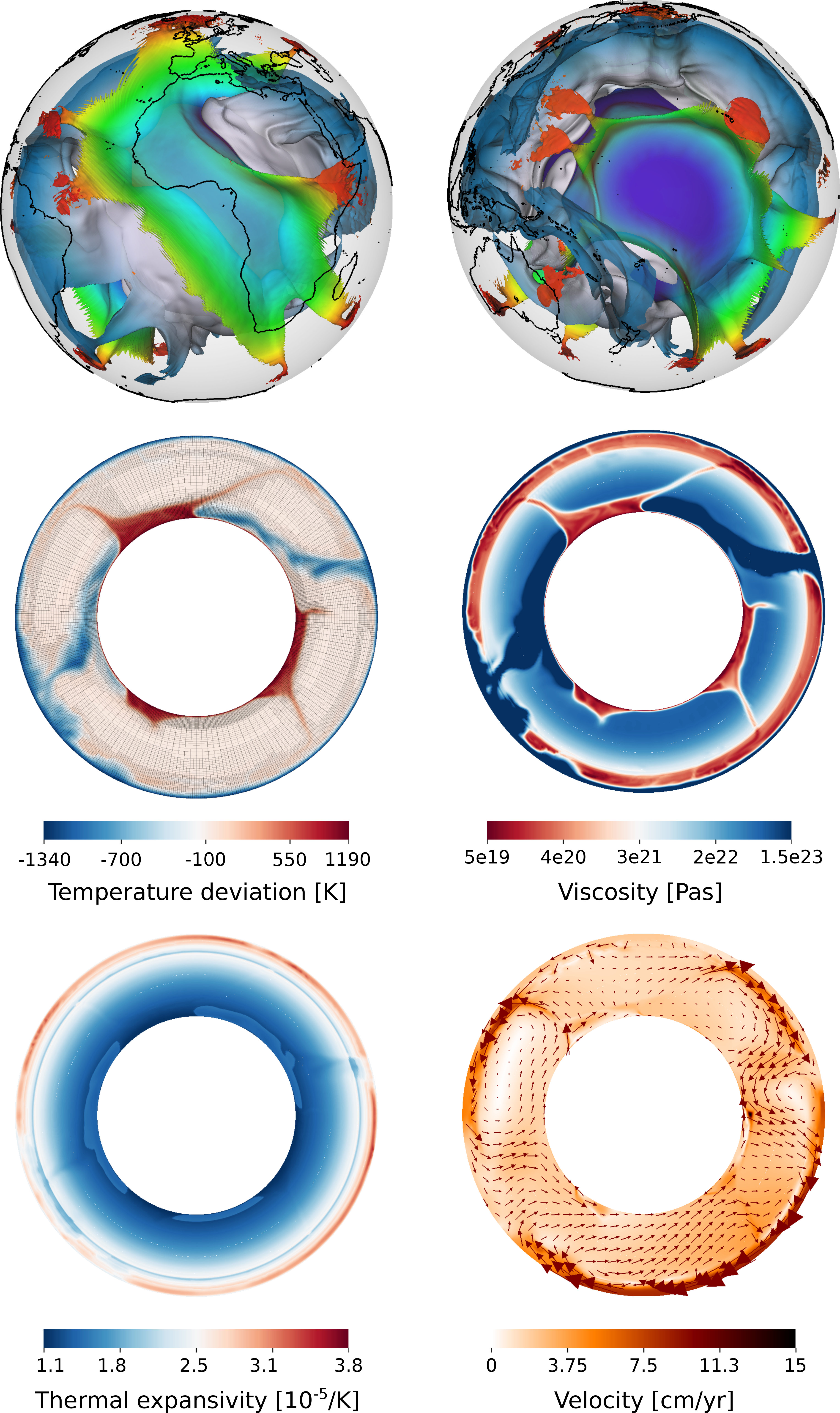 Figure 1
 Figure 2
 Figure 3
 Figure 4
 Figure 5
 Figure 6
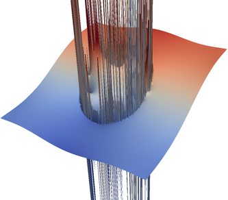 Figure 7
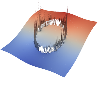 Figure 8
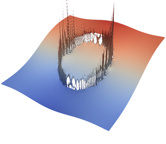 Figure 9
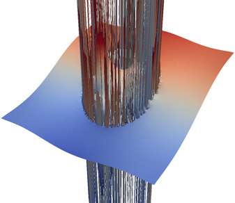 Figure 10
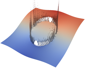 Figure 11
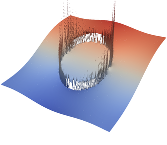 Figure 12
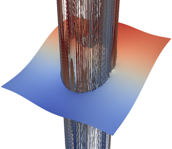 Figure 13
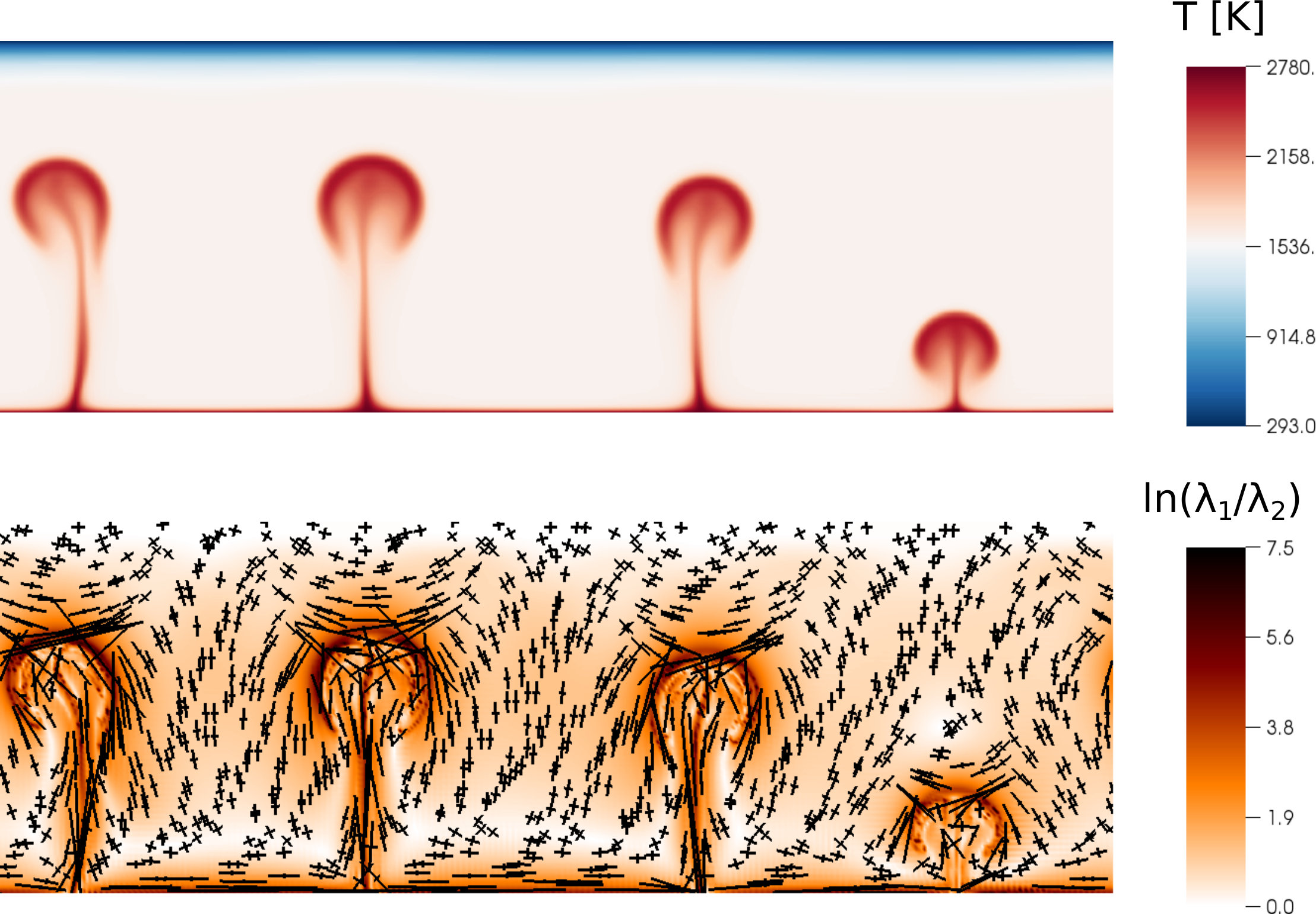 Figure 14
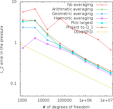 Figure 15
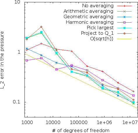 Figure 16
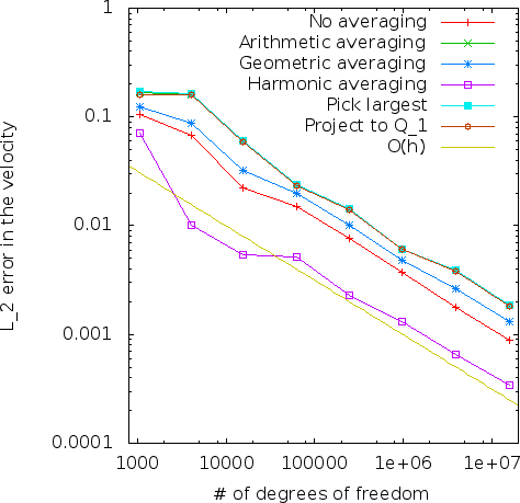 Figure 17
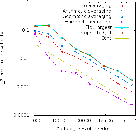 Figure 18
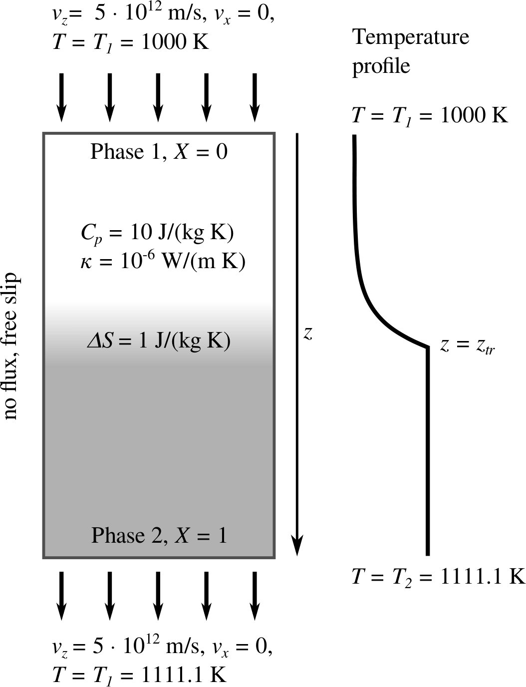 Figure 19
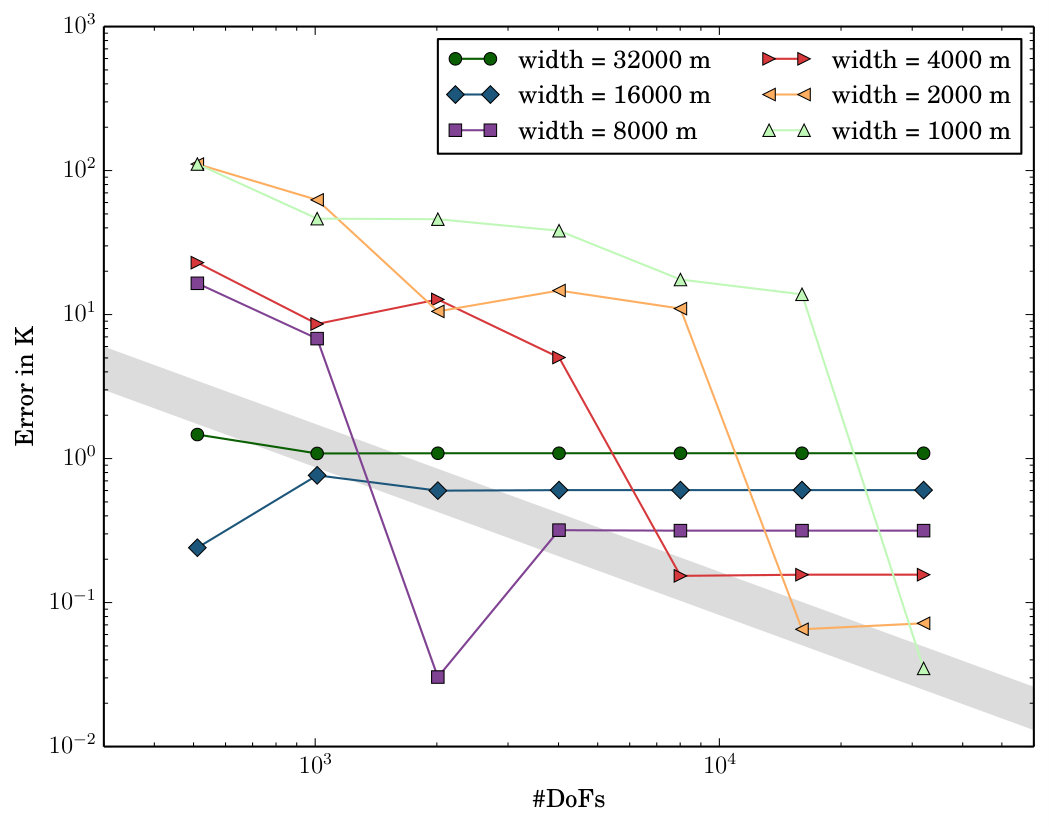 Figure 20
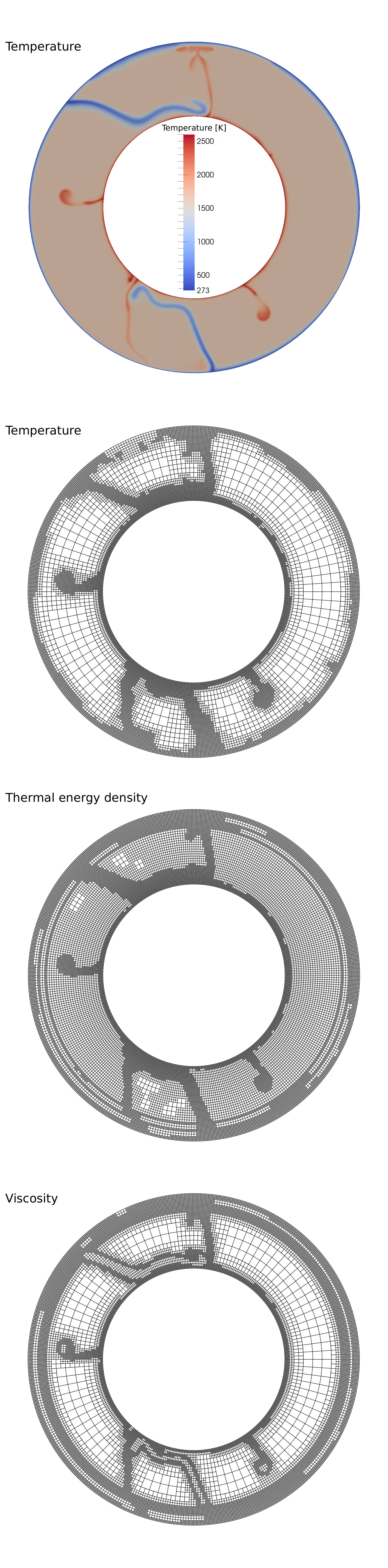 Figure 21
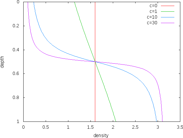 Figure 22
| implicit | |||||
|---|---|---|---|---|---|
| Mesh | DoFs | ||||
| 9539 | 43 | 43 | 52 | 64 | |
| 37507 | 46 | 48 | 62 | 75 | |
| 148739 | 50 | 52 | 65 | 72 | |
| 592387 | 56 | 62 | 79 | 114 | |
| explicit | |||||
| Mesh | DoFs | ||||
| 9539 | 43 | 125 | 257 | 334 | |
| 37507 | 46 | 133 | 289 | 388 | |
| 148739 | 50 | 132 | 267 | 328 | |
| 592387 | 56 | 140 | 303 | 407 | |
| explicit (first nonlinear iteration) | |||||
| Mesh | DoFs | ||||
| 9539 | 43 | 43 | 43 | 43 | |
| 37507 | 46 | 46 | 46 | 46 | |
| 148739 | 50 | 50 | 50 | 50 | |
| 592387 | 56 | 56 | 56 | 56 | |
| 1/h | rate | |||
| Boussinesq approximation (BA) | ||||
| 8 | 9.0721e-06 | - | ||
| 16 | 1.1103e-06 | 3.03 | ||
| 32 | 1.3806e-07 | 3.01 | ||
| 64 | 1.7242e-08 | 3.00 | ||
| Truncated anelastic liquid approximation (TALA), | ||||
| 8 | 1.2109e-05 | - | 4.5439e-07 | 2.2179e-07 |
| 16 | 1.4840e-06 | 3.03 | 2.9067e-08 | 1.4130e-08 |
| 32 | 1.8459e-07 | 3.01 | 1.6974e-09 | 5.5979e-10 |
| 64 | 2.3056e-08 | 3.00 | 6.2599e-11 | 2.9021e-10 |
| Truncated anelastic liquid approximation (TALA), | ||||
| 8 | 8.7973e-06 | - | 2.1267e-07 | 1.4399e-07 |
| 16 | 1.1207e-06 | 2.97 | 1.3707e-08 | 9.3239e-09 |
| 32 | 1.4078e-07 | 2.99 | 8.0734e-10 | 4.9389e-10 |
| 64 | 1.7638e-08 | 3.00 | 2.6633e-12 | 6.6108e-11 |
| Expression | Value | |
|---|---|---|
| temperature change across the domain | 3000 K | |
| surface temperature | 273 K | |
| Grueneisen parameter | 1 | |
| width and height of the box | 1 m | |
| gravitational acceleration in negative z direction | 1 m s-2 | |
| thermal expansivity | Di | |
| specific heat | 1 J kg-1 K-1 | |
| surface density | 1 kg m-3 | |
| viscosity | Di/Ra | |
| thermal conductivity | 1 W m-1 K-1 |
| Di | Ra | Nu | Vrms | W | |||
|---|---|---|---|---|---|---|---|
| 0.25 | Aspect | 4.4145 | 39.9568 | 0.5149 | 0.8496 | 0.849 | |
| King UM | 4.406 | 39.952 | 0.515 | 0.847 | 0.849 | ||
| King VT | 4.4144 | 40.0951 | 0.5146 | 0.849 | 0.849 | ||
| King CU | 4.41 | 40 | 0.5148 | 0.8494 | 0.8501 | ||
| 1 | Aspect | 2.446 | 24.6809 | 0.5114 | 1.3427 | 1.354 | |
| King UM | 2.438 | 24.663 | 0.512 | 1.343 | 1.349 | ||
| King VT | 2.4716 | 25.0157 | 0.51 | 1.3622 | 1.3621 | ||
| King CU | 2.47 | 24.9 | 0.5103 | 1.3627 | 1.3638 | ||
| 0.25 | Aspect | 9.2334 | 178.0751 | 0.5322 | 2.0525 | 2.0517 | |
| King UM | 9.196 | 178.229 | 0.532 | 2.041 | 2.051 | ||
| King VT | 9.2428 | 179.7523 | 0.5318 | 2.0518 | 2.0519 | ||
| King CU | 9.21 | 178.2 | 0.5319 | 2.0503 | 2.054 | ||
| 1 | Aspect | 3.8699 | 84.3678 | 0.5298 | 2.7519 | 2.7692 | |
| King UM | 3.857 | 84.587 | 0.53 | 2.742 | 2.765 | ||
| King VT | 3.878 | 85.5803 | 0.5294 | 2.761 | 2.7614 | ||
| King CU | 3.88 | 84.6 | 0.5294 | 2.7652 | 2.7742 |
| Mesh size | No averaging | Arithmetic | Harmonic |
|---|---|---|---|
| averaging | averaging | ||
| 60 | 25 | 20 | |
| 89 | 24 | 22 | |
| 129 | 24 | 24 | |
| 138 | 26 | 24 | |
| 277 | 25 | 25 |
| Di | Ra | 1/h | Nu | Vrms | W | ||
|---|---|---|---|---|---|---|---|
| 0.25 | 16 | 4.53819 | 40.02007 | 0.51514 | 0.85213 | 0.85157 | |
| 0.25 | 32 | 4.45192 | 39.96357 | 0.51496 | 0.84984 | 0.84928 | |
| 0.25 | 64 | 4.42482 | 39.95753 | 0.51494 | 0.84960 | 0.84903 | |
| 0.25 | 128 | 4.41735 | 39.95684 | 0.51494 | 0.84957 | 0.84901 | |
| extrapolated | 4.41450 | 39.95676 | 0.51494 | 0.84957 | 0.84900 | ||
| 0.25 | King UM | 4.406 | 39.952 | 0.515 | 0.847 | 0.849 | |
| 0.25 | King VT | 4.4144 | 40.0951 | 0.5146 | 0.849 | 0.849 | |
| 0.25 | King CU | 4.41 | 40 | 0.5148 | 0.8494 | 0.8501 | |
| 0.5 | 16 | 3.91228 | 35.98789 | 0.52271 | 1.38719 | 1.38541 | |
| 0.5 | 32 | 3.84891 | 35.94470 | 0.52245 | 1.38402 | 1.38225 | |
| 0.5 | 64 | 3.82932 | 35.93997 | 0.52241 | 1.38368 | 1.38190 | |
| 0.5 | 128 | 3.82399 | 35.93943 | 0.52241 | 1.38364 | 1.38187 | |
| extrapolated | 3.82200 | 35.93936 | 0.52241 | 1.38363 | 1.38186 | ||
| 0.5 | King UM | 3.812 | 35.936 | 0.522 | 1.381 | 1.381 | |
| 0.5 | King VT | 3.8218 | 36.0425 | 0.5214 | 1.3812 | 1.3812 | |
| 0.5 | King CU | 3.82 | 35.9 | 0.5217 | 1.3818 | 1.383 | |
| 1 | 16 | 2.47804 | 24.69538 | 0.51160 | 1.34460 | 1.35568 | |
| 1 | 32 | 2.45507 | 24.68259 | 0.51145 | 1.34286 | 1.35415 | |
| 1 | 64 | 2.44835 | 24.68113 | 0.51143 | 1.34270 | 1.35399 | |
| 1 | 128 | 2.44659 | 24.68096 | 0.51142 | 1.34268 | 1.35398 | |
| extrapolated | 2.44596 | 24.68094 | 0.51142 | 1.34268 | 1.35397 | ||
| 1 | King UM | 2.438 | 24.663 | 0.512 | 1.343 | 1.349 | |
| 1 | King VT | 2.4716 | 25.0157 | 0.51 | 1.3622 | 1.3621 | |
| 1 | King CU | 2.47 | 24.9 | 0.5103 | 1.3627 | 1.3638 | |
| 0.25 | 16 | 9.83522 | 179.93650 | 0.53284 | 2.09314 | 2.09246 | |
| 0.25 | 32 | 9.53887 | 178.40376 | 0.53247 | 2.05964 | 2.05880 | |
| 0.25 | 64 | 9.33472 | 178.11210 | 0.53220 | 2.05331 | 2.05248 | |
| 0.25 | 128 | 9.26701 | 178.07926 | 0.53216 | 2.05260 | 2.05177 | |
| extrapolated | 9.23341 | 178.07510 | 0.53216 | 2.05251 | 2.05168 | ||
| 0.25 | King UM | 9.196 | 178.229 | 0.532 | 2.041 | 2.051 | |
| 0.25 | King VT | 9.2428 | 179.7523 | 0.5318 | 2.0518 | 2.0519 | |
| 0.25 | King CU | 9.21 | 178.2 | 0.5319 | 2.0503 | 2.054 | |
| 0.5 | 16 | 8.02846 | 156.42656 | 0.54891 | 3.28922 | 3.28780 | |
| 0.5 | 32 | 7.77804 | 155.33598 | 0.54847 | 3.24554 | 3.24386 | |
| 0.5 | 64 | 7.63386 | 155.14464 | 0.54809 | 3.23782 | 3.23615 | |
| 0.5 | 128 | 7.58838 | 155.12248 | 0.54805 | 3.23693 | 3.23526 | |
| extrapolated | 7.56741 | 155.11957 | 0.54804 | 3.23682 | 3.23514 | ||
| 0.5 | King UM | 7.532 | 155.304 | 0.548 | 3.221 | 3.233 | |
| 0.5 | King VT | 7.5719 | 156.5589 | 0.5472 | 3.2344 | 3.2346 | |
| 0.5 | King CU | 7.55 | 155.1 | 0.5472 | 3.233 | 3.2392 | |
| 1 | 16 | 4.01908 | 84.62206 | 0.53004 | 2.77354 | 2.78862 | |
| 1 | 32 | 3.91951 | 84.38966 | 0.52998 | 2.75378 | 2.77104 | |
| 1 | 64 | 3.88354 | 84.37059 | 0.52983 | 2.75208 | 2.76937 | |
| 1 | 128 | 3.87364 | 84.36817 | 0.52981 | 2.75189 | 2.76918 | |
| extrapolated | 3.86988 | 84.36782 | 0.52980 | 2.75187 | 2.76916 | ||
| 1 | King UM | 3.857 | 84.587 | 0.53 | 2.742 | 2.765 | |
| 1 | King VT | 3.878 | 85.5803 | 0.5294 | 2.761 | 2.7614 | |
| 1 | King CU | 3.88 | 84.6 | 0.5294 | 2.7652 | 2.7742 |
| Di | Ra | 1/h | Nu | Vrms | W | ||
|---|---|---|---|---|---|---|---|
| 0.25 | 16 | 4.54966 | 40.11121 | 0.51292 | 0.85535 | 0.85306 | |
| 0.25 | 32 | 4.46241 | 40.05425 | 0.51276 | 0.85304 | 0.85075 | |
| 0.25 | 64 | 4.43490 | 40.04816 | 0.51274 | 0.85279 | 0.85050 | |
| 0.25 | 128 | 4.42730 | 40.04747 | 0.51273 | 0.85277 | 0.85047 | |
| extrapolated | 4.42440 | 40.04738 | 0.51273 | 0.85276 | 0.85047 | ||
| 0.25 | King UM | 4.416 | 40.043 | 0.513 | 0.85 | 0.85 | |
| 0.25 | King VT | 4.43 | 40.2 | 0.5127 | 0.8535 | 0.851 | |
| 0.25 | King CU | 4.42 | 40.1 | 0.5129 | 0.8539 | 0.8521 | |
| 0.5 | 16 | 3.95543 | 36.36149 | 0.51906 | 1.41082 | 1.39596 | |
| 0.5 | 32 | 3.88987 | 36.31653 | 0.51882 | 1.40750 | 1.39267 | |
| 0.5 | 64 | 3.86941 | 36.31161 | 0.51879 | 1.40714 | 1.39232 | |
| 0.5 | 128 | 3.86383 | 36.31105 | 0.51879 | 1.40710 | 1.39228 | |
| extrapolated | 3.86173 | 36.31098 | 0.51879 | 1.40710 | 1.39227 | ||
| 0.5 | King UM | 3.851 | 36.307 | 0.519 | 1.404 | 1.391 | |
| 0.5 | King VT | 3.86 | 36.4 | 0.5188 | 1.41 | 1.393 | |
| 0.5 | King CU | 3.86 | 36.3 | 0.5191 | 1.4103 | 1.3948 | |
| 1 | 16 | 2.60286 | 26.04904 | 0.50879 | 1.46096 | 1.40373 | |
| 1 | 32 | 2.57654 | 26.03180 | 0.50864 | 1.45907 | 1.40188 | |
| 1 | 64 | 2.56869 | 26.02986 | 0.50862 | 1.45886 | 1.40168 | |
| 1 | 128 | 2.56661 | 26.02964 | 0.50862 | 1.45883 | 1.40166 | |
| extrapolated | 2.56586 | 26.02961 | 0.50862 | 1.45883 | 1.40165 | ||
| 1 | King UM | 2.556 | 26.007 | 0.509 | 1.459 | 1.396 | |
| 1 | King VT | 2.57 | 26.1 | 0.5088 | 1.465 | 1.4 | |
| 1 | King CU | 2.57 | 26 | 0.5092 | 1.4651 | 1.4019 | |
| 0.25 | 16 | 9.85211 | 180.27625 | 0.53099 | 2.09904 | 2.09486 | |
| 0.25 | 32 | 9.55792 | 178.73582 | 0.53064 | 2.06534 | 2.06106 | |
| 0.25 | 64 | 9.35214 | 178.44234 | 0.53038 | 2.05898 | 2.05470 | |
| 0.25 | 128 | 9.28366 | 178.40932 | 0.53035 | 2.05826 | 2.05399 | |
| extrapolated | 9.24951 | 178.40514 | 0.53034 | 2.05817 | 2.05390 | ||
| 0.25 | King UM | 9.211 | 178.56 | 0.53 | 2.046 | 2.053 | |
| 0.25 | King VT | 9.26 | 180.2 | 0.5303 | 2.06 | 2.055 | |
| 0.25 | King CU | 9.23 | 178.6 | 0.5303 | 2.0597 | 2.0573 | |
| 0.5 | 16 | 8.09115 | 157.65389 | 0.54628 | 3.32727 | 3.30146 | |
| 0.5 | 32 | 7.84156 | 156.53900 | 0.54587 | 3.28255 | 3.25680 | |
| 0.5 | 64 | 7.69385 | 156.34222 | 0.54551 | 3.27460 | 3.24890 | |
| 0.5 | 128 | 7.64696 | 156.31949 | 0.54546 | 3.27368 | 3.24800 | |
| extrapolated | 7.62514 | 156.31653 | 0.54545 | 3.27357 | 3.24788 | ||
| 0.5 | King UM | 7.588 | 156.503 | 0.545 | 3.258 | 3.245 | |
| 0.5 | King VT | 7.63 | 157.93 | 0.5454 | 3.279 | 3.25 | |
| 0.5 | King CU | 7.61 | 156.5 | 0.5455 | 3.2779 | 3.2552 | |
| 1 | 16 | 4.07456 | 85.14137 | 0.52985 | 2.83063 | 2.77505 | |
| 1 | 32 | 3.97234 | 84.89394 | 0.52980 | 2.81369 | 2.75800 | |
| 1 | 64 | 3.93521 | 84.87353 | 0.52966 | 2.81193 | 2.75626 | |
| 1 | 128 | 3.92499 | 84.87099 | 0.52964 | 2.81173 | 2.75606 | |
| extrapolated | 3.92110 | 84.87063 | 0.52964 | 2.81170 | 2.75604 | ||
| 1 | King UM | 3.907 | 85.105 | 0.529 | 2.802 | 2.75 | |
| 1 | King VT | 3.92 | 86.08 | 0.5297 | 2.821 | 2.757 | |
| 1 | King CU | 3.92 | 85.1 | 0.5297 | 2.8278 | 2.7725 |
Peer Reviews
No public reviews on file for this paper yet. If you reviewed it on a platform where reviews are public (OpenReview, ICLR, NeurIPS, ICML), you can paste yours below so the community can read it here.
Videos
No videos yet. Explain this paper in a talk, walkthrough, or lecture? Add one.
High Accuracy Mantle Convection Simulation through Modern Numerical
Methods. II: Realistic Models and Problems
Timo Heister1
Juliane Dannberg2 Now at Department of Mathematics, Colorado State University, Fort Collins, CO 80523-1874.
Rene Gassmöller3
Wolfgang Bangerth4
1 *Mathematical Sciences, Clemson University, O-110 Martin Hall, Clemson, SC 29634-0975, USA; [email protected]
2 Department of Mathematics, Texas A&M University, Mailstop 3368, College Station, TX 77843-3368, USA; [email protected]
3 Department of Mathematics, Colorado State University, Fort Collins, CO 80523-1874, USA; [email protected]
4 Department of Mathematics, Colorado State University, Fort Collins, CO 80523-1874; [email protected] *
Abstract
Computations have helped elucidate the dynamics of Earth’s mantle for several decades already. The numerical methods that underlie these simulations have greatly evolved within this time span, and today include dynamically changing and adaptively refined meshes, sophisticated and efficient solvers, and parallelization to large clusters of computers. At the same time, many of these methods – discussed in detail in a previous paper in this series [Kronbichler et al.(2012)] – were developed and tested primarily using model problems that lack many of the complexities that are common to the realistic models our community wants to solve today.
With several years of experience solving complex and realistic models, we here revisit some of the algorithm designs of the earlier paper and discuss the incorporation of more complex physics. In particular, we re-consider time stepping and mesh refinement algorithms, evaluate approaches to incorporate compressibility, and discuss dealing with strongly varying material coefficients, latent heat, and how to track chemical compositions and heterogeneities. Taken together and implemented in a high-performance, massively parallel code, the techniques discussed in this paper then allow for high resolution, 3d, compressible, global mantle convection simulations with phase transitions, strongly temperature dependent viscosity and realistic material properties based on mineral physics data.
Keywords: Mantle convection, numerical methods, adaptive mesh refinement, finite element method, compressibility, preconditioners
NOTE: This paper has been published in Geophysical Journal International with the title “High Accuracy Mantle Convection Simulation through Modern Numerical Methods. II: Realistic Models and Problems” with identifier https://dx.doi.org/10.1093/gji/ggx195.
1 Introduction
Computer simulations are at the heart of most attempts at understanding the dynamics of the Earth’s mantle as well as the interiors of other celestial bodies. As such, there is a long tradition in the investigation of numerical methods that help us solve the equations that describe mantle convection, dating back many decades (e.g. [Torrance & Turcotte(1971), Richter(1973), McKenzie et al.(1974), Baumgardner(1985), Tackley et al.(1993)], see also [May et al.(2013)] and references therein). Many of these articles parallel the general development of computational science methods, and have moved from simple, low-order, uniform 2d mesh discretizations with fixed-point linear solvers, to using adaptively refined, dynamically changing 3d meshes with higher order elements and complicated linear and nonlinear solvers [Stadler et al.(2010), Alisic et al.(2010), Davies et al.(2011), Burstedde et al.(2013), Gerya et al.(2013), Rudi et al.(2015)]. Indeed, a previous paper [Kronbichler et al.(2012)] in the current series of publications was devoted to the description of current, state-of-the-art methods for mantle convection simulations.
At the same time, most of these methods – including the ones in our earlier paper – were developed, tested, and evaluated using relatively simple model problems (e.g. [Blankenbach et al.(1989), Busse et al.(1993), van Keken et al.(1997), Tackley & King(2003), Schmeling et al.(2008), van Keken et al.(2008), Zhong et al.(2008), King et al.(2010), Crameri et al.(2012), Tosi et al.(2015)]). Yet, this no longer matches what our community wants to do today: We want to solve more realistic problems that use compressible formulations with discontinuous coefficients, for example. We also want to use more complex geometries, possibly varying with time. And we may want to include other physical effects such as latent heat, the transport of chemical inhomogeneities or tracking of tensor quantities like finite strain. For these kinds of applications, we have found that the numerical methods currently used in our community often perform worse than for the traditional model problems and benchmarks.
The purpose of this paper is therefore to revisit the traditional choices of numerical methods for mantle convection in light of complex applications. Specifically, we will consider how time stepping, mesh refinement, formulations for compressible materials, and other aspects of computational codes are affected when they are applied to complex problems. In some cases, previous methods perform poorly and need to be adapted; in others, previous methods were simply unsuitable, and we are faced with a variety of choices that allow us to design algorithms that are both well suited to the problem as well as allow for accurate and fast solutions.
We base our discussions on the five years of experience we have with the Aspect code111The “Advanced Solver for Problems in Earth ConvecTion”, an open source project to provide a modern, parallel, extensible code to simulate mantle convection. Aspect’s development is supported by the Computational Infrastructure for Geodynamics initiative, as well as by the National Science Foundation. See http://aspect.dealii.org. since we described many of these methods in [Kronbichler et al.(2012)]. In this time, we and others have applied Aspect to more complex and realistic problems [Austermann et al.(2015), Tosi et al.(2015), Rose et al.(2017), Gassmöller et al.(2016), Dannberg & Heister(2016), Zhang & O’Neill(2016), He et al.(2016)], and the discussions in the remainder of this paper reflect the challenges encountered in this process. On the other hand, the discussions herein are not specific to Aspect: They are about the general design of numerical methods for the problems at hand, and apply equally to any other code that wants to solve them.
We intend this contribution to be of interest to those designing their own numerical methods for mantle convection, but also for those interested in understanding more about how modern mantle convection codes work. Finally, some of the sections below outline open problems that call for more methodological or mathematical research; the paper should therefore also be of interest to the numerical methods and numerical analysis community as it outlines areas requiring better methods.
The remainder of this paper is structured as follows: Section 2 first lays out the general mathematical formulation of the problem we want to consider. Section 3 then discusses how time stepping methods need to be adjusted to more complex problems (Section 3.1); how approaches can be designed to deal with compressibility (Section 3.2), averaging discontinuous coefficients (Section 3.3), and latent heat (Section 3.4); how mesh refinement can be made to deal with realistic applications (Section 3.5); and approaches to advecting along additional quantities (Section 3.6). We show results for a large and complex application in Section 4, and conclude in Section 5.
2 Formulation of the problem
Within this paper, let us consider a model for the flow of a compressible, anelastic fluid, such as generally assumed for convection in the Earth’s mantle (e.g. [Schubert et al.(2001)]). Flow is driven by buoyancy due to thermal or compositional gradients, and the model includes the effects of friction and adiabatic heating, radiogenic heat production and latent heat on the energy balance. However, the model ignores inertial and elastic effects as we are concerned with very low velocities and long time scales. Specifically, let us consider the following set of equations:
[TABLE]
In this system of equations, denotes the fluid velocity, the pressure, and the temperature. For the stress we have with the rate-of-deformation tensor .
In the equations above, and are the effective viscosity, density, and specific heat capacity of the material. , , and are the thermal conductivity, intrinsic specific heat production, thermal expansion coefficient, gravity vector, and entropy, respectively. is the material derivative of the entropy of a volume of material, and will be discussed in Section 3.4. We will in the following assume that all of these parameters with the exception of gravity can depend on the current temperature and pressure; furthermore, we allow that can depend on the strain rate and that all parameters may also depend on the location to facilitate material parametrisations that are not derived from realistic material models but incorporate a priori modeling assumptions. In other words, we will henceforth consider , , , , , . Note that we assume the anelastic conservation of mass equation (2) and only consider the density to be a dependent variable of temperature, pressure, and location; in particular, we neglect the time derivative and thus elastic waves, see [Schubert et al.(2001)] for details.
In the remainder of this paper, we will make no assumptions that coefficients are continuous. In fact, we explicitly allow parameters to jump discontinuously as commonly happens when using thermodynamically consistent models that incorporate phase changes. Indeed, it is these kinds of difficulties that set apart the model problems often considered, from the kind of problems that are the subject of this paper.
There are numerous approximations to equations (1)–(3) that have been widely used in the literature, such as the anelastic liquid approximation (ALA), truncated anelastic liquid approximation (TALA) and Boussinesq approximation (BA), see for example [Bercovici et al.(1992), Schubert et al.(2001), King et al.(2010), Tan & Gurnis(2007)]. These can all be derived by assuming that density variations are small compared to the hydrostatic density increase. We will discuss differences between these approximations and (1)–(3) in Section 3.2, but these differences are not fundamental to this paper: Any numerical issues that may arise from describing the complex phenomena we aim to model would arise using any of the above formulations; consequently, the solution strategies we derive are useful for all those cases.
3 Numerical methods
As discussed in the introduction, the goal of this section is to outline areas where the numerical methods commonly employed for model or simplified problems run into difficulties when applied to more complex formulations and problems. The methods we compare against are Taylor-Hood finite elements to discretize the Stokes equations, along with a block-preconditioned GMRES solver for the resulting linear equations. The temperature equation is also discretized using the finite element method; the advection is stabilized via the addition of a nonlinear entropy viscosity. The entire set of equation is discretized on adaptively refined, dynamically changing meshes in 2d or 3d. All of these methods are described in detail in a previous paper [Kronbichler et al.(2012)]. We consider them state-of-the-art within the computational mantle convection community.
The focus of the following subsections is, then, on the modifications necessary as one moves from simpler, model problems to the more realistic description of convective transport in the Earth’s mantle provided in the previous section. Specifically, we will discuss time stepping; dealing with compressibility; averaging of discontinuous coefficients; incorporating latent heat; mesh adaptation; and advection schemes for additional quantities. On the other hand, we will not elaborate on the solution of models with non-linear, strain-rate dependent rheologies; a discussion and extensive benchmarking of such cases can be found in [Glerum et al.(2017)].
All computations in this section are done using the open source mantle convection code Aspect [Kronbichler et al.(2012), Bangerth et al.(2017b)], which builds on deal.II [Bangerth et al.(2016)], p4est [Burstedde et al.(2011)], and Trilinos [Heroux et al.(2005)]; our test computations were done with Aspect version 1.5.0 [Bangerth et al.(2017a)] and the setups for all computations are available at https://github.com/tjhei/paper-aspect-methods-2-data.
3.1 Time stepping for the temperature equation revisited:
explicit, semi-implicit, implicit
In [Kronbichler et al.(2012)], we have advocated for a semi-implicit method for the time discretization of the temperature equation (3). In this approach, one treats the thermal diffusion term implicitly, but the advection term explicitly. This choice guarantees that only the advection term implies a stability limit for the size of the time step . In particular, the corresponding Courant-Friedrichs-Lewy (CFL) condition states that the time discretized problem is only stable if we choose , where is a measure of the (one-dimensional) size of cell , the polynomial degree of the finite element used to discretize the temperature field, and is the maximal velocity on cell . is a constant related to the time stepping method; it always satisfies if some terms of the equation are treated explicitly, and generally becomes smaller with increasing convergence order of the chosen time stepping method.
In pursuing this strategy, we were motivated by two observations. First, the matrix that needs to be inverted in solving the temperature equation with this choice of terms treated implicitly yields a symmetric and positive definite matrix for which efficient solution methods are readily available, in particular the Conjugate Gradient method combined with multigrid preconditioners. Second, while fully implicit methods may choose time steps much larger than and still remain stable, we typically want to choose the time step around anyway for accuracy reasons because this guarantees that information is not transported across more than the distance between adjacent nodes within one time step. This is of increasing importance when using adaptive mesh refinement.
However, in applying this approach to more realistic problems, one encounters two difficulties:
- •
How exactly should be defined?
- •
How large or small does one have to choose ?
These questions are relatively easy to answer on uniform meshes for rectangular or box-shaped meshes. There, all possible definitions of – either (i) the diameter of cell , (ii) the shortest edge of , (iii) the minimal distance between any two vertices, (iv) the square or cube root of the volume of the cell in 2d and 3d, respectively – are all equivalent up to a fixed constant and any choice is valid as long as the constant is appropriately adjusted. After choosing any of these definitions, we can determine a safe value for experimentally.
On the other hand we desire to solve problems on complex domains that will include cells of varying shapes; examples are meshes that discretize models on shell segments, but also may have a free top boundary and/or describe real topology. In such meshes, the various ways of defining what is, are no longer equivalent up to a fixed constant, and it is not clear what definition is the most appropriate to allow for the largest choice of time steps.
Secondly, it may require extensive test simulations to determine whether a particular choice of leads to a stable scheme because a solution may only “blow up” once steep features of the solution happen to pass a particularly poorly shaped cell, rather than such a steep feature simply existing.
The consequence of all of this is that in practice, one needs to choose rather small to guarantee stability in all circumstances. As stated in [Kronbichler et al.(2012)], we needed to choose in 2d and in 3d. For any larger value, we could find geometries and problem setups for which the temperature eventually became instable, even though the resulting time steps are almost certainly smaller than necessary for most other cases.
Such small time steps are impractical in practice. While the resulting solution is stable, it is not significantly more accurate than if we had chosen a fully implicit method with . However, using the semi-implicit scheme for the temperature equation is vastly more expensive: we need as many time steps for the semi-implicit method (i.e., roughly one sixth of the number of time steps in 2d, and less than one fortieth in 3d), each including solving both the Stokes and the temperature equation.
For these reasons, we have come to believe that the better choice for the time stepping scheme is a fully implicit time discretization – for example a BDF-2 scheme to discretize the term – in which we choose and to be the minimal distance between any two vertices of cell . Because this choice treats advection implicitly, it results in a system matrix that is no longer symmetric and positive definite. This requires more costly solvers and preconditioners, for example GMRES instead of CG. On the other hand, this effort is vastly over-compensated by the fact that we have reduced the number of time steps by a factor of more than 5 (in 2d) or 40 (in 3d). Furthermore, even the fully implicit temperature solver requires less than 10% of the overall run time in realistic simulations; in other words, having to choose a less efficient linear solver due to the addition of a non-symmetric term does not affect the overall computational cost of each time step in a significant way. What determines the overall computational cost of a simulation, however, is how many time steps we have to solve.
3.2 Compressibility
Incorporating compressibility into existing codes is likely the most difficult issue when moving from model problems to realistic descriptions of Earth. This is because compressibility makes the mass conservation equation (2) nonlinear, or adds additional terms when using the ALA or TALA approximation. Furthermore, the divergence term is no longer adjoint to the gradient of the pressure, and depending on how it is treated numerically, the matrix resulting from the Stokes equation after discretization may no longer be symmetric. As a consequence, how exactly one deals with the compressibility has significant implications for how nonlinear and linear solvers need to be written and will perform. On the other hand, there are significant opportunities for algorithm design whereby one can choose different re-formulations based on which of these allows for efficient and accurate implementations. The next sub-section (Section 3.2.1) will therefore be about the various trade-offs involved, before we comment on considerations of the symmetry of resulting solvers (Section 3.2.3), making the right hand sides of linear systems compatible (Section 3.2.2), and finally show numerical results illustrating several of the points previously discussed (Sections 3.2.4 and 3.2.5).
Various forms of compressibility have been incorporated into mantle convection codes for several decades already, though often only for particular formulations such as the ALA or TALA in which the density in the mass conservation equation is explicitly prescribed as a function of depth. We refer to [Baumgardner(1985), Tan & Gurnis(2007), Leng & Zhong(2008), Tackley(2008), King et al.(2010)] for details on how other codes deal with these issues.
3.2.1 Reformulating the compressible Stokes equations
Solving compressible models numerically poses a number of challenges. First, the mass conservation equation given in (2), is nonlinear if depends on the solution variables and has to be linearised. Secondly, any linearised version results in an operator that is no longer adjoint to the term in the force balance equation, resulting in a non-symmetric matrix with consequences for the construction of efficient solvers and preconditioners for the linear system. This second issue also arises for any approximation of equations (1)–(2) that includes a non-constant density in the mass balance equation, for example the (truncated) anelastic liquid approximation (T)ALA [King et al.(2010)]. Because of this universal importance, we will discuss the difficulties that result from compressible models in some detail in the following.
There are a number of possible avenues for linearisation of (2). For example, one could instead use the equation
[TABLE]
where is a known approximation of the density that is computed from the previous time step’s temperature and pressure, or from a temperature and pressure that has been extrapolated from previous time steps to the current time, and might be updated during a nonlinear iteration. Alternatively, in the case of the (T)ALA, simply is a prescribed density profile that does not change over time. In all those cases, may still be spatially variable, but it no longer depends on the quantities that we are currently solving for. While this resolves the nonlinearity, the operator is not adjoint to the gradient operator acting on the pressure in the force balance equation; direct discretizations of this term therefore do not lead to a symmetric system matrix.
In addition, the term is not computable in practice because the product is not a finite element function (or other polynomial) of which we can compute derivatives during assembly. One way to make it computable is to multiply out the divergence. In order to make the equation look similar to the one we have in the incompressible case, we also divide by the density. Two choices that result from this are then to consider either222Both of these methods are also implemented in the widely used code CitcomS [Zhong et al.(2008)], though we are not aware of a systematic discussion of the two options, nor of comprehensive tests of their differences as we provide below.
[TABLE]
or
[TABLE]
In the last equation, we have also frozen the velocity in the right hand side term to a fixed value obtained from previous time steps. If depends on the pressure, either of these approaches then require a nonlinear iteration to converge to the desired solution.
These two formulations are also not without difficulty. First, the replacement strictly only makes sense if the density is continuous. If it is not, for example when taking into account phase changes, then is a continuous function of which we can take derivatives, whereas we cannot of its components and .333This is, however, a theoretical consideration since the finite element spaces we use will not allow us to represent discontinuous velocities anyway. While the traditional approach to dealing with undesirable derivatives is to multiply with test functions and integrate by parts, this is not possible here because the pressure test functions with which this equation is multiplied are only in and consequently not sufficiently smooth to allow for integration by parts.
Second, there are also difficulties from the perspective of finite element approximations when using a density that depends on the primary variables pressure and temperature (and possibly other variables such as the chemical composition) in equation (4) or (5). In this case, and likewise, for the finite element approximation (indicated by the index ), . On the other hand, the theory of the Stokes equations yields that in general, the pressure is only a function in , see for example [Ern & Guermond(2004)]. In practice, this means that one does not usually get a better approximation than for the finite element approximation of the pressure, unless the solution happens to be smooth. Indeed, if the viscosity is discontinuous or has large gradients, one often gets an even lower convergence order; for example, the SolCx test case yields a convergence order (see [Kronbichler et al.(2012)]). This implies that, assuming we use a continuous finite element space to approximate the pressure, we can at best hope that converges to as in some average sense, but that we can not expect this to happen with any particular order; in other words, the best one might hope for is a statement of the form , but the approximation will likely be very poor and probably not converge in a pointwise sense. (Indeed, we demonstrate this experimentally in Section 3.3.) Pointwise convergence can obviously not be expected at all if one uses discontinuous finite element spaces for the approximation of the pressure. Consequently, any practical scheme that replaces by terms that include will likely yield a rather poorly approximated density gradient, resulting in degradation in convergence of the velocity and temperature. We therefore would like to avoid the occurrence of in our scheme.
To this end, we replace . This is motivated by the observation that for the hydrostatic pressure that dominates the total pressure in the Earth mantle, by definition we have with the adiabatic reference density ; indeed, in the (T)ALA approximations, one chooses . We can then approximate . Using this allows us to re-state the equations above as
[TABLE]
or
[TABLE]
In the following, we will call these two options the implicit and explicit approximation, because they either include the velocity implicitly or explicitly in the term that contains the gradient of the pressure.
Both of these approximations introduce errors that depend on (i) how accurately approximates , which can be controlled by small time steps and accurate extrapolations from previous time steps; and (ii) how good the approximation for is, which is related to how small the velocity is, and consequently how appropriate the choice of the equations (1)–(2) was to begin with. The more relevant question is therefore which of these approximations one wants to use for practical considerations.
To understand this, it is instructive to recall that discretizations of the force balance equation (1) together with the approximations (6), and (7) lead to system matrices with the following structure:
[TABLE]
Which one we choose has consequences for available choices of linear solvers and preconditioners that are important since in most realistic simulations, 70% or more of the overall run time is spent in solving the discretized velocity-pressure system. Furthermore, since we linearise the equation we really want to solve, we will have to iterate out the nonlinearity, and the two choices will require different numbers of outer, nonlinear iterations. Predictably, the choice that keeps the velocity entirely implicit, (6), and can therefore be expected to converge more quickly in the nonlinear iteration, will also lead to more difficult-to-solve linear systems due to the lack of symmetry. Consequently, the choice between (6) and (7) is not a priori clear.
3.2.2 Correcting the right hand side
When using the explicit approximation (7), we end up with an equation that is rank deficient if the fluid flow is enclosed in a domain where the normal component of the fluid velocity is prescribed on all parts of the boundary (a typical example being either no-slip or tangential flow). In those cases, integrating over the domain and using the divergence theorem yields
[TABLE]
The left hand side of this equation is fixed and known based on the given boundary conditions. On the other hand, the right hand side may be whatever it is, based on our choice of approximations as well as the choice of quadrature formula and geometric approximation of the domain. Thus, it may or may not equal the fixed value on the left, and if it does not, then (7) will not allow for a solution. On the other hand, it is clear that the difference between the two sides will be small if are well chosen and if the assumptions that went into (7) are valid. Thus, we can make the system solvable again by replacing (7) by the equation
[TABLE]
where is chosen so that the invariant is always satisfied:
[TABLE]
This correction is easily computed before assembling the linear system that results from the linearisation of the Stokes equation, and amounts to slightly correcting the compressibility everywhere to ensure global mass conservation.
We note that in the case of an incompressible material, we have , and mass conservation of course implies that the sum of influxes and outfluxes has to balance, i.e., . Consequently, for incompressible materials, always evaluates to zero; no correction is necessary in this case. (However, for inhomogeneous boundary conditions one has to be more careful, see [Heister et al.(2016)].) Likewise, if the material is compressible but the setup of the problem has a part of the boundary where only a normal stress of the fluid is prescribed, then fluid velocity and pressure can adjust independently to allow any right hand side to the mass conservation equation, and the correction above is neither necessary nor desirable.
3.2.3 Cost evaluation of the two formulations
It is not a priori clear which of the two formulations, (6) or (8), is preferable from a practical perspective: The first is “more implicit” and consequently likely requires fewer nonlinear iterations; the second yields a symmetric system matrix and consequently likely requires fewer linear GMRES iterations because we can formulate a better preconditioner.444A discussion of the preconditioner we use can be found in [Kronbichler et al.(2012)]. Specifically, for linear systems of the form we use the preconditioner proposed by Silvester and Wathen for the symmetric Stokes system (see [Silvester & Wathen(1994), Elman et al.(2005)] for a derivation): where a tilde indicates an approximation and is the Schur complement of the symmetric part. This preconditioner does not include the matrix and can therefore be expected to deteriorate if the compressibility in the implicit formulation becomes large. We have spent a significant amount of time testing preconditioners that include in some way, but have not been able to find ones that improve on the one shown above.
To resolve the question, we have performed a number of numerical experiments.
Specifically, our test problem consists of a unit box, uses the truncated anelastic liquid approximation (TALA), and a spatially variable adiabatic density of the form
[TABLE]
where we will vary the coefficient that describes the deviation from a constant density in the set (see Fig. 1). The density’s derivative has a peak at with . We use the non-dimensional Rayleigh number and dissipation number , and prescribe constant inflow at the top boundary, , free slip at left and right boundaries, and open outflow at the bottom.
We show a comparison of the number of GMRES iterations in Table 1. The numbers there show that indeed a single implicit solve (using (6)) is more expensive in terms of GMRES iterations than a single explicit solve (using (8)) for all choices of the compressibility parameter. In fact, iterations for a single solve of the explicit formulation are independent of . On the other hand, the explicit formulation requires a Picard iteration to iterate the nonlinearity, and the number of linear GMRES iterations accumulated over these Picard iterations is significantly larger than for the implicit formulation.
The result of these experiments is that for stationary computations, the implicit formulation is both computationally cheaper and, likely, more stable. On the other hand, for time dependent problems the explicit formulation may be cheaper since one will already have a good approximation for and one may only need a single nonlinear iteration.
3.2.4 Benchmark for the compressible Stokes flow solver
We have verified our implementations of the compressible Stokes and temperature formulations (Section 3.2.1) using a number of benchmarks. In particular, we have reproduced the results from the community benchmark described in [King et al.(2010)] (see Section 3.2.5). We have also reproduced the benchmark given in the Appendix of [Tan & Gurnis(2007)] and will describe our results in the following. This latter benchmark consists of an analytical solution for an instantaneous compressible Stokes flow problem (with a given temperature). Using Fourier decomposition, the problem can be reduced to a boundary value ordinary differential equation that can be solved numerically up to machine precision.
The test case in [Tan & Gurnis(2007)] is defined in terms of the non-dimensional Rayleigh and dissipation numbers,
[TABLE]
where a characteristic length scale, a characteristic temperature difference, a reference density, and all other parameters as introduced in Section 2. We then use the benchmark in the form discussed in [Tan & Gurnis(2007)], but with equation (B4) corrected to read
[TABLE]
We implement the benchmark in the setting of equations (1)–(3) by fixing all of the above material constants to , except for and . We then test both the Boussinesq approximation (BA) and the truncated anelastic liquid approximation (TALA), and compute the error of the velocity, and errors of the integrals of shear () and adiabatic heating (). The problem is instantaneous, so we perform a nonlinear iteration with the explicit formulation of the compressibility for a single timestep. Alternatively, one can use the implicit formulation and perform a single Stokes solve, which gives very similar results.
The results are shown in Table 2 and show optimal third order convergence for the error of the velocity. Both heating terms show less regular, but equally fast convergence to the exact values, with the total shear heating converging at an even higher order than the velocity.
3.2.5 Benchmark for 2d Cartesian compressible convection
In order to verify that our approaches to solving compressible problems also work for more complex applications, we also evaluate the correctness and accuracy of the re-formulations of the equations introduced in Section 3.2.1 using the community benchmark defined in [King et al.(2010)]. The model domain for this benchmark is a 2-D square box cooled from the top and heated from the bottom. This setup corresponds to the benchmark given in [Blankenbach et al.(1989)], except that the material is no longer assumed to be incompressible and instead different approximations for the compressible mass conservation equation are tested. All material properties are approximated as constants, with the exception of the density, which varies around a reference state
[TABLE]
A constant temperature is prescribed at the top () and bottom () of the domain, with
[TABLE]
and no flux conditions at the side walls. This temperature increase across the model domain includes both the contribution of the adiabatic temperature profile,
[TABLE]
and the nonadiabatic temperature variations across the boundary layers. The initial temperature is a linear profile that matches these boundary conditions, plus a small perturbation:
[TABLE]
We then let the model evolve until steady state is reached.
Analogous to the procedure described in Section 3.2.4, we reproduce the non-dimensional formulation of the benchmark by setting all material constants to 1, except for and . In the different benchmark cases, Di is varied between and , and Ra is chosen as and . All parameters are given in Table 3.
We have tested both the anelastic liquid approximation (ALA) and the truncated anelastic liquid approximation (TALA) using our reference implementation of our algorithms in the Aspect code [Kronbichler et al.(2012)]. Because we are only interested in the steady-state limit, rather than accurate intermediate values, we report results for the explicit formulation (7) with the modification in (8), without actually iterating out the nonlinearity in every time step. (However, we have also verified that the implicit formulation, (6), yields essentially the same results.) Table 4 provides an excerpt of results for the ALA, with full results for both ALA and TALA given in Tables 6 and 7. Specifically, we compare the Nusselt number Nu, root mean square velocity , average temperature , the total shear heating and adiabatic heating to the results given in [King et al.(2010)]. As can be seen from the table, there is excellent agreement between our results and those previously reported. In other words, the re-formulations in Section 3.2.1 do not only allow us to efficiently solve compressible problems, but also accurately.
3.3 Averaging of material properties
Geophysical models are often characterized by abrupt and large jumps in material properties, in particular in the viscosity. An example is a subducting, cold slab surrounded by the hot mantle: Here, the strong temperature-dependence of the viscosity will lead to a sudden jump in the viscosity between mantle and slab. Another example are phase transitions, where the density and viscosity of rocks change abruptly between the stability field of different minerals. The length scale over which this happens will be a few or a few tens of kilometres. Such length scales cannot be adequately resolved in three-dimensional computations with typical meshes for global computations. In other words, the viscosity field is, for all practical purposes, discontinuous, with jumps of possibly several orders of magnitude from quadrature point to quadrature point.
Having large viscosity variations in models poses a variety of problems to numerical computations. First, they lead to very long compute times because solvers and/or preconditioners break down (see [Rudi et al.(2015)] for a proposed preconditioner for large viscosity variations). This may be acceptable if it would at least lead to accurate solutions, but large viscosity variations also lead to large pressure gradients, and this in turn leads to over- and undershoots in the numerical approximation of the gradient. We will demonstrate both of these issues experimentally in Section 3.3.2 and 3.3.3 below.
One can mitigate some of these effects by averaging material properties in some form on each cell (see, for example, [Schmeling et al.(2008), Deubelbeiss & Kaus(2008), Duretz et al.(2011), Thieulot(2015), Thielmann et al.(2014)]). At the same time, replacing the correct viscosity at each quadrature point by an averaged one implies solving a different problem, and one would expect this to affect the accuracy of the solution. In cases where the viscosity (and consequently the solution) is smooth, averaging could be assumed to be harmful to the overall accuracy. On the other hand, if the solution has essentially discontinuous gradients and kinks in the velocity field, then at least at these locations we cannot expect a particularly high convergence order anyway, and the averaging will likely not hurt very much either. This section therefore explores these issues and shows numerical results.
3.3.1 Implementation
In implementations, averaging first evaluates the material model at every quadrature point of a cell, given the temperature, pressure, strain rate, and other quantities at these points, and then either (i) uses these values as is in the assembly of contributions to the system matrix and right hand side, or (ii) replaces the values by their arithmetic average , harmonic average , geometric average , or largest value over all quadrature points on this cell. Alternatively, one may project the values from the quadrature points to a bi- (in 2d) or trilinear (in 3d) finite element space on every cell, and then evaluate this finite element representation again at the quadrature points; in this case, one may also limit the computed values at quadrature points by the minimum and maximum value of the coefficient before averaging. These operations are applied to all quantities that the material model computes, i.e., in particular, the viscosity, the density, the compressibility, and the various thermal and thermodynamic properties.
A priori, we know of little guidance from the literature on the analysis of numerical discretizations of partial differential equations regarding the question which of these averaging options is best. Indeed, it is also not quite clear what the appropriate metric would be to determine “best” – for example, one could consider various norms of the errors, run time of solvers, or other metrics. Consequently, in the following sections we will consider a simple test case and evaluate the options above with regard to discretization error and the time necessary to solve the linear system associated with each.
3.3.2 Influence of averaging on numerical accuracy
We experimentally evaluate the question which of the introduced averaging operations may in fact be best by considering the “sinker” benchmark. This benchmark is defined by a high-viscosity, heavy disk at the center of a two-dimensional box. Both density and viscosity are therefore discontinuous along the interface of the disk, and in particular not aligned with the mesh. We use outside the disk, and inside the disk to simulate a realistic viscosity contrast; the contrast in the density is immaterial as it is only a (global) scaling factor for the solution.
For three of the averaging options introduced above, and for different levels of mesh refinement, Fig. 2 shows pressure plots that illustrate the problem with oscillations of the discrete pressure, without and with averaging. The important part of these plots is not that the solution looks discontinuous – in fact, the exact solution is discontinuous at the edge of the circle – but the spikes that go far above and below the “cliff” in the pressure along the edge of the circle. Without averaging, these spikes are far larger than the actual jump height. Importantly, the spikes also do not disappear under mesh refinement nor averaging; in other words, the discrete pressure does not converge in the norm to the exact pressure. (Further investigations also show that the maximal and minimal pressures continue to grow with mesh refinement, although slowly, with or without averaging.) On the other hand, the pressure spikes become far less pronounced with averaging.
The results shown in the figure do not allow to draw definitive conclusions as to which averaging approach is the best. This is in line with previous discussions of this question, for example in [Schmeling et al.(2008), Deubelbeiss & Kaus(2008), Duretz et al.(2011), Thielmann et al.(2014)]). On the other hand, we can investigate this by evaluating the error in the solution for the closely related “Pure shear/Inclusion” benchmark (see [Duretz et al.(2011)]) for which we know the exact solution. To this end, Fig. 3 shows the errors in velocity and pressure for a variety of averaging options and as meshes are refined. The figures clearly show that all averaging schemes improve the pressure approximation, though some deteriorate the velocity approximation. In light of Figures 2 and 3, using harmonic averaging appears to be a reasonable compromise. This is again in agreement with previous statements in the literature.
One may follow the problem with discontinuous pressures in a different direction and suggest that the pressure could be better approximated by using a discontinuous pressure space. This is in fact possible for the Stokes equations, by choosing a discontinuous pressure space instead of the common continuous space of the Taylor-Hood pair, without losing the inf-sup stability of the discrete problem [Kronbichler et al.(2012)]. Disappointingly, however, this makes no real difference: the pressure oscillations are no better (in fact, they are worse) than for the standard Stokes element (Fig. 4) and the errors are generally worse for both velocity and pressure (Fig. 5).
3.3.3 Influence of averaging on solver speed
A very pleasant side effect of averaging is that solutions are not only better behaved, but are also cheaper to compute. For example, the total run time for the sinker testcase of the previous section (see Fig. 2), using a mesh and the Taylor-Hood element, is reduced from 5870s without averaging to 240s for harmonic averaging – a speed-up of a factor of around 25!
Such improvements carry over to more complex and realistic models. For example, in a simulation with large viscosity heterogeneities using approximately 17 million unknowns and run on 64 processors, the wall-clock run time is reduced from 145 hours to 17 hours and the computed solutions do not differ in any significant way.
We attempt to quantify this effect in Table 5 by looking at the number of outer GMRES iterations necessary to solve the variable viscosity Stokes system. We use a preconditioner equations that involves an inner solver with an algebraic multigrid preconditioner for the elliptic top-left block of the matrix (corresponding to the “expensive” option discussed in [Kronbichler et al.(2012)]). Using this scheme, the number of GMRES iterations rises steeply with mesh refinement without averaging, see Table 5. On the other hand, with (any kind of) averaging, the number of iterations remains much lower. The effect is even more dramatic when using the discontinuous pressure element mentioned in the previous section: there, without averaging, the number of iterations grows from 389 on a mesh to 1174 on a mesh, while the number of iterations with averaging are very similar to those shown in Table 5.
We can also quantify how many fewer outer GMRES iterations one needs with averaging for the complex model mentioned above: There, the number of iterations is reduced from 169 to 77.
However, the number of outer GMRES iterations is only part of the problem. Depending on the choice of preconditioner for the Stokes system, one has to also iteratively invert the elliptic top-left block of the Stokes matrix, and/or a pressure mass matrix. These “inner” solves also become vastly cheaper with averaging, requiring 2 to 5 times fewer Conjugate Gradient iterations than without averaging per preconditioner application. Together with the reduction in outer iterations, overall run time for the Stokes solver is reduced by the factors discussed at the beginning of the subsection.
3.4 Latent heat
When incorporating phase transitions into realistic mantle convection models we are not only faced with abrupt changes of material properties across these transitions as discussed in Section 3.3, but also with a relatively sudden change in internal energy of the material. This means that latent heat is consumed or released over a sharp interface as material crosses a particular phase boundary. In the energy balance (3), this is expressed as a heating term describing the changes of the entropy in terms of its material derivative. As the entropy of a given material depends only on temperature and pressure (assuming a constant chemical composition), we can rewrite the corresponding heating term in (3) as
[TABLE]
Together with the approximation that the fluid is anelastic (see Section 2) – that is, assuming – and when moving all advection terms involving the temperature to the left-hand side, the energy balance (3) can be rewritten in the following form:
[TABLE]
3.4.1 Implementation
Different approaches for how to implement this equation have been suggested in the literature:
One may describe a number of prominent phase transitions using the Clapeyron slope , density change and an analytic phase function , such as a hyperbolic tangent, that describes the stability field of each phase and varies between 0 and 1,
[TABLE]
see for example [Christensen & Yuen(1985)]. 2. 2.
One may use a thermodynamic calculation package, such as Perple_X [Connolly(2009)] or BurnMan [Cottaar et al.(2014)] to compute - tables of material properties, including the enthalpy (or its pressure and temperature derivatives), which describes the energy changes associated with phase transitions. Between data points of these tables, one may then interpolate continuously (yielding a smoothed out approximation of the true - diagram) and compute derivatives and based on this interpolation. 3. 3.
One may use a modified version of (ii) that involves using the pressure and temperature derivatives of the enthalpy to compute an “effective” thermal expansivity
[TABLE]
and specific heat
[TABLE]
respectively, which are then used in the energy conservation equation in place of the original quantities and account for latent heat effects (see for example [Nakagawa et al.(2009)]).
All of these methods have in common that they introduce relatively narrow regions where latent heat is consumed or released. Even though phase changes generally occur over a range of pressures and temperatures, and are also not instantaneous, their width is often below the grid resolution of geodynamic computations. Hence, strategies have to be designed for smoothing out sharp transitions so that they can be treated numerically, but still yield a high accuracy. In addition, narrow zones of latent heat release lead to strong temperature gradients with consequent difficulties for numerical schemes that have to be addressed by stabilization as discussed in [Kronbichler et al.(2012)].
3.4.2 Numerical results
We numerically evaluate the reformulation of latent heat processes in (11) by using the benchmark described in [Schubert et al.(2001), part 1, p. 194]. It provides an analytical solution for the latent heat that is released or consumed when material undergoes a phase transition. An important consideration in practice is to assess by how much the temperature can deviate from the correct solution if the phase transition is not properly resolved. Our experiments are therefore targeted at estimating how many mesh cells across a phase transition are required to accurately model the temperature change.
The basic setup is a pipe with prescribed material inflow at constant velocity and temperature at the top, outflow at the bottom, and a univariant phase transition (occurring at a single value of temperature and pressure) approximately in the center of the domain (Fig. 6). As initial condition, the model uses a uniform temperature field; however, when material crosses the phase transition, latent heat is released.
In the steady state limit, this leads to a temperature profile with a higher temperature in the bottom half of the domain, which can be calculated by solving the energy equation (equation (11), using approach (i) above) for one-dimensional downward flow with (constant) vertical velocity :
[TABLE]
Here, with the thermal conductivity and the thermal diffusivity. The latent heat generation is the product of the temperature , the entropy change across the phase transition divided by the specific heat capacity and the derivative of the phase function , which indicates the fraction of material transitioned from phase 1 to phase 2. If the velocity is smaller than a critical value (see also [Schubert et al.(2001)] part 1, pp. 193–195), this latent heat term will be zero everywhere except for the one depth where the phase transition occurs discontinuously.
This means that there are two one-phase regions, one above with only phase 1, and one below with only phase 2, where the equation above (using the boundary conditions for and for ) can be solved as
[TABLE]
As we consider only the steady state, and the solution given above tells us that for (the region downward of the phase transition) the temperature is constant (see also the temperature profile in Fig. 6), there is no net downward transport of heat from the phase change interface. In other words, the amount of heat generated at the phase transition is the same as the heat conducted upwards from the transition:
[TABLE]
Rearranging this equation and using gives
[TABLE]
In the numerical model, we can not exactly reproduce the behaviour of a Dirac delta function as would result from taking the derivative of the discontinuous phase function that is considered in the benchmark. Rather, we use a hyperbolic tangent with a (small) finite width to model . This leads to a deviation of the numerical from the analytical solution that is dependent on how well the mesh resolves the transition zone and how large one chooses the transition zone width to be. Both the mesh size and the width of the transition zone can be chosen independently for numerical purposes.
Fig. 7 shows numerical results that demonstrate this interplay: If the resolution is high enough to resolve the phase boundary (which requires approximately 4 mesh cells across the phase transition, using bi-quadratic finite elements, in our experiments), the error is small and is dominated by the phase transition width – the deviation of the approximate, smoothed model from the exact one. On the other hand, while the mesh is too coarse to resolve the transition zone, neither mesh refinement nor reducing the size of the transition zone have a significant effect.
Hence, for modeling discontinuous phase transitions (or phase transitions that are too narrow to be resolved in the numerical model), to reach the highest accuracy the phase transition width should be chosen as approximately four times of the smallest cell size. This corresponds to the first data point after the kink of each line in Fig. 7, i.e. the area highlighted in gray, thus demonstrating predictable convergence.
3.5 Mesh refinement
Many finite element codes supporting adaptive mesh refinement use the “Kelly” refinement criterion [Gago et al.(1983)] to refine and coarsen the mesh in response to the computed solution (for an overview of other error indicators used in computational geodynamics simulations, we refer to [May et al.(2013), Burstedde et al.(2013), Davies et al.(2011)]). In the case of time-dependent problems such as the one discussed here, one would perform this adaptation every few time steps. The “Kelly” criterion computes a numerical approximation to the second derivative of a finite element function , times a power of the mesh size, by evaluating for every cell the quantity
[TABLE]
where denotes the jump of the enclosed quantity across the interface between cell and its neighbours, is the normal vector to the boundary of cell , and is the diameter of .
This criterion was originally developed as an error estimator for the Laplace equation [Kelly et al.(1983)], but has been found widely useful in adaptive meshing because it also estimates the polynomial interpolation error on every cell. It has thus been used for many different equations to generate good meshes, even if no provably accurate error estimators are available for these equations.
In the context of mantle convection, it therefore seems appropriate to drive mesh refinement by applying this criterion to either the temperature or velocity field. Indeed, we advocated for this approach in [Kronbichler et al.(2012)] based on the observation that this should help reduce the error in the natural energy norms for these two solution variables.
On the other hand, in actual applications, one is often interested in a variety of quantities that are, at best, tangentially related to the energy norm error and whose approximation is not always improved by choosing a mesh based on an energy error indicator. A typical example would be simulations that investigate the importance of phase changes on the dynamics of convection: While the coefficients in the equations (e.g., density, viscosity) and possibly other derived quantities such as seismic velocities are discontinuous at these interfaces, the solution fields (e.g., temperature and velocity) may vary in ways that do not make such interfaces obvious. Consequently, only refining based on velocity and temperature may not yield meshes that reveal these phase boundaries in sufficient detail to really capture their small-scale influences. Furthermore, the meshes so generated would not allow to extract interfaces with sufficient resolution to account for the dynamic effects of phase changes, latent heat transfer as discussed in Section 3.4, or for comparison against observations like seismic tomographic models.
3.5.1 A practical approach
Despite the fact that we have well over a decade of experience with mesh adaptation algorithms, it is not clear to us how one can devise methods that automatically take into account what one may be interested in. Dual Weighted Residual methods such as those discussed in [Bangerth & Rannacher(2003)] may be appropriate but are unwieldy to implement for time-dependent problems. Instead, the best solution we can come up with is a complex but flexible, two-tiered system for adaptive mesh refinement that is primarily driven by letting users choose what information they think is most important for their purposes. In a first step, we compute refinement indicators by choosing among a list of indicators that include the following:
- •
The “Kelly” indicator applied to the velocity or temperature.
- •
A weighted discrete approximation of the gradient,
[TABLE]
Here, is the center of , the space dimension, and the factor is chosen so that indicators converge to zero as the mesh size even for discontinuous discretizations of otherwise continuous exact solutions . This criterion is then applied to derived quantities such as the density, the viscosity, or the thermal energy density .
The criteria are then scaled or normalized to yield , and the final refinement indicators are obtained by either computing the maximum of (scaled or normalized) error indicators, , or the sum of these indicators, . Cells are then marked for coarsening or refinement based on .
There are also cases where refinement needs to be driven algorithmically, rather than based on criteria derived from solution or derived values. For example, we have found that it is often useful to only refine in a region of particular interest, even though the model is larger; in these cases, one can think of the larger model (with a relatively coarse mesh) as providing self-consistent boundary values for the smaller region of interest (with a finer mesh). Another example is to ensure a minimal refinement level for all cells at the surface, or at a particular depth.
This approach provides great flexibility in defining how and where the mesh is refined, as necessary, and thereby provide high accuracy where it is important for the particular question one wants to investigate in a simulation. At the same time, there is little theoretical underpinning that this approach is “optimal” (however one may want to define this).
3.5.2 Mesh refinement in 2-D spherical convection
We demonstrate the flexibility provided by the mesh refinement procedure using an example of 2D mantle convection that includes phase transitions and the associated discontinuities of density and viscosity. The geometry is a spherical shell, and the mantle is heated from the bottom, where the temperature is fixed to 2600 K, and cooled from the top, where the temperature is 273 K. No additional heating processes (such as shear heating, adiabatic heating, or latent heat) are included, and the initial temperature is constant at 1600 K except for the two thermal boundary layers.
We model two phase transitions at depths of 410 km and 660 km (reflecting the olivine-spinel and spinel-perovskite transformations), where both viscosity and density change discontinuously. Specifically, we use a viscosity
[TABLE]
where Pa s in the upper mantle, Pa s between 410 km and 660 km depth, and Pa s in the lower mantle; we choose the dimensionless activation energy , and the reference temperature K.
Our density model satisfies
[TABLE]
with kg/m3, Pa-1, K-1, and density increases of kg/m3 and kg/m3 at the 410 km and 660 km phase transitions. Velocities at the outer boundary are prescribed, using the present-day plate velocities along the equator projected onto the two-dimensional slice used in our model [Gurnis et al.(2012)].
Fig. 8 shows the temperature distribution in this model after 260 million years, together with the corresponding meshes generated using different criteria for the adaptive refinement. The figure illustrates how a refinement criterion based solely on the temperature almost entirely misses the phase transitions in favour of resolving only the boundary layers and plumes. It would therefore not yield sufficiently resolved fields for comparisons with tomographic models of Earth. On the other hand, refining based on weighted approximate gradients of either the thermal energy density or the viscosity allows the resolution of phase boundaries.
Which of these meshes yields the “best” solution cannot be quantified without specifying what the “goal” of the simulation is. It is possible that the meshes refined based on the thermal energy density or the density have a larger energy norm error in the velocity and/or temperature. On the other hand, their accuracy in predicting tomographically visible interfaces is certainly much higher.
3.6 Tracking chemical compositions and other quantities
In many complex simulations of mantle convection, it is necessary to track not only the flow of thermal energy (described by equation (3)), but also how the chemical composition, trace or radiogenic elements, isotope ratios, water content – or other quantities such as grain sizes – are transported along with the velocity.
In mantle convection codes, this has traditionally (and successfully) be done using tracer particles [Poliakov & Podladchikov(1992), Gerya & Yuen(2003), McNamara & Zhong(2004), Popov & Sobolev(2008), Thielmann et al.(2014)]. However, it is not trivial to implement tracers efficiently and scalably in the context of large-scale parallel codes with dynamically changing, adaptively refined meshes, as opposed to globally refined, statically partitioned, fixed meshes. A number of these challenges – and possible solutions – are discussed in more details in [Gassmoeller et al.(2016)].
On the other hand, many of the applications that have traditionally motivated the use of particles can equally well be done by using a field-based description of the quantities one wants to advect along. The advantage in using this approach is the well developed numerical infrastructure for solving advection equations, and the ease with which these can then be evaluated at quadrature points when computing material properties; highly efficient tools are also available in many of the available finite element libraries to facilitate data movement upon mesh refinement and repartitioning (see, for example, [Bangerth et al.(2011)]).
Using field-based approaches then requires advecting any number of “compositional fields” along with the velocity field, by solving the advection equations
[TABLE]
where are source terms that may depend on velocity, pressure, temperature, and the compositional fields themselves. Through appropriate choices of these source terms, one can also model reactions among fields, for example to describe compositional changes upon partial melting or freezing of material. On the other hand, entirely different reactions can equally easily be modelled, and we will outline one example in Section 3.6.2 below.
In practice, the compositional fields are easily evaluated at quadrature points, and can therefore be used to affect the description of material parameters such as the density and viscosity.
3.6.1 Implementation
As stated, equation (14) does not contain any diffusion, in line with the fact that chemical species do not diffuse at appreciable rates on length scales of the Earth mantle. Consequently, the numerical solution of (14) presents challenges when modeling sharp gradients – for example, when tracking chemical heterogeneities, or when using the fields to track where material that originates from one particular area is transported over time. To stabilize the numerical solution, one typically employs one of many artificial viscosity schemes, such as the SUPG formulation [Brooks(1981), Brooks & Hughes(1982)] or schemes based on the residual of an entropy equation [Guermond et al.(2011), Kronbichler et al.(2012)]. This is of course also necessary for the temperature equation (3).
In practical applications, it has proven useful to allow descriptions of the source terms that may consist both of finite but time dependent components, and of impulse functions in time. An example for the use of impulse functions is where the describe the chemical composition of rocks; if these compositions change due to partial melting and melt extraction that happen instantaneously (compared to the size of a time step) as a rock moves through the phase diagram, the compositions also need to change instantaneously, rather than continuously. Allowing both continuous and impulse components can be achieved by providing the functions that compute with current values of strain rate, temperature, pressure, compositions, and spatial location, along with a time increment , and require them to return . If contains impulse components, then the functions’ return value will simply have a contribution that is not proportional to .
3.6.2 Tracking finite strain
We demonstrate the flexibility of using compositional fields using the example of a Cartesian convection model that tracks the accumulated finite strain at every location of the domain. For this purpose, we define as the components of the deformation gradient (or deformation) tensor , which represents the deformation accumulated over time by idealized little grains of finite size. This is done in such a way that (in 2D) , , etc. The time derivative of can be computed as
[TABLE]
where is the velocity gradient tensor [McKenzie & Jackson(1983), Dahlen & Tromp(1998), Becker et al.(2003)]. The initial deformation is , with being the identity tensor.
This means that the on the right-hand side of Equation (14) can be computed as the product of the current velocity gradient and the accumulated deformation at the previous time step.
A direct visualization of is not intuitive, because it contains rotational components that represent a rigid body rotation without deformation. Following [Becker et al.(2003)] we can polar-decompose the tensor into a positive-definite and symmetric tensor , and an orthogonal rotation tensor , as , therefore . The left stretching tensor then describes the deformation we are interested in, and its eigenvalues and eigenvectors describe the length and orientation of the half-axes of the finite strain ellipsoid. Moreover, we will represent the amount of relative stretching at every point by the ratio , called the natural strain [Ribe(1992)].
The model we present here as an example for tracking of finite strain features a box with an aspect ratio of three and dimensions of 2900 8700 km. The mantle is cooled from the top (where the temperature is 293 K) and heated from the bottom (where the temperature is 2780 K) with no additional heat sources in the form of internal heating or latent heat. The density is modelled as
[TABLE]
with kg m-3, K-1 and the reference temperature K. Thermal conductivity and gravity are set to W m-1 K-1 and m s-2. We choose the temperature-dependent viscosity as
[TABLE]
with Pa s and . Hence, the bottom thermal boundary layer, where viscosities are lower, becomes unstable first, and plumes start to rise towards the surface, see Fig. 9 (top). Material moves to the sides at the top of the plume head, so that it is shortened in vertical direction (short black vertical lines in Fig. 9, bottom) and stretched in horizontal direction (long horizontal lines). The sides of the plume head show the opposite effect. Shear occurs mostly at the edges of the plume head, in the plume tail, and in the bottom boundary layer (black areas in the natural strain distribution).
4 Application to a complex problem
In order to present the methods discussed in the previous sections in practice, we here show results of a global mantle convection model that combines a compressible formulation with earth-like material properties, a strongly temperature dependent viscosity, chemical heterogeneities tracked by compositional fields, and prescribed surface velocities.
In particular, the model geometry resembles Earth’s mantle, and starts from an undisturbed, motionless state. A layer of dense basaltic material with initially uniform thickness of km covers the core-mantle boundary, and the initial temperature profile follows an adiabat of K computed with the material properties that are provided by the Perple_X software [Connolly(2005)] based on a database of mineral properties [Stixrude & Lithgow-Bertelloni(2011)], overall a method similar to [Nakagawa et al.(2009)]. This approach yields realistic, earth-like material properties, but also entails several challenges, such as discrete sampling in pressure–temperature space, and quasi-discontinuous jumps due to phase transitions. The viscosity is based on a published viscosity model incorporating constraints from mineral physics, geoid deformation and seismic tomography [Steinberger & Calderwood(2006)]. It is depth- and temperature dependent with a depth-dependent activation enthalpy of – kJ/mol and would lead to viscosity variations of at least eight orders of magnitude over the model temperature range. In order to limit the maximal velocity, and thus the number of timesteps and computational cost, we artificially restrict the viscosity to the range – Pa s by cutting off values outside of this range. As has been shown elsewhere, see [Dannberg & Heister(2016), Tosi et al.(2015)], our Stokes solver is capable of solving larger viscosity contrasts up to at least seven orders of magnitude. Surface velocities in the model are prescribed using published plate reconstructions [Seton et al.(2012)], and are prepared by the GPlates software [Boyden et al.(2011)] at discrete positions, and interpolated to the adaptively refined mesh within Aspect. Boundary temperatures are prescribed to K (at the surface) and K (at the core-mantle boundary). The resolution of the finest mesh cells is 23 km (large portions of the model are adaptively coarsened), and the overall computation has about 100 million degrees of freedom in each time step. The model requires 3,700 time steps, within which we iterate out the nonlinearity with on average about 2 sub-iterations (for a total of 6,000 nonlinear iterations). The model required a computing time of 24.5 hours on 1536 processes, i.e., 37,600 CPU hours.
The model results presented in Fig. 10 demonstrate the complexities that arise in realistic mantle convection models as discussed in this paper. The strongly temperature dependent viscosity leads to narrow upwelling plumes (with diameters around 100 km) that rise from the edges of the dense basal piles and reach the surface close to observed hotspot locations on Earth as observed in many other studies [Steinberger & Torsvik(2012), Davies et al.(2012), Bower et al.(2013), Hassan et al.(2015)]. Due to its low viscosity the plume material moves with velocities larger than cm/yr in the upper mantle thus limiting the timestep length of the model. The mineral physics based material properties contain sharp gradients in density, thermal expansivity, and specific heat capacity; these are particularly prominent in the mantle transition zone and at the Bridgmanite-Postperovskite transition close to the core-mantle boundary in the lower left panel of Fig. 10.
The more complex setup of our model compared to earlier studies – including compressibility, highly temperature-dependent viscosity, and more complex material parameters – does not change the basic results of the computation. However, the setup focuses the plumes into narrower structures, and the higher accuracy possible with our methods allows additional use cases for the model results: Velocities, temperature and compositions can be used as constraints for regional high-resolution models investigating particular processes such as the interaction between rising mantle plumes and mid-ocean ridges [Gassmöller et al.(2016)], or the generation and ascent of chemically zoned plumes that are thought to be responsible for the generation of zoned hotspot tracks [Weis et al.(2011)]. Consistent temperature and pressure profiles of compressible models also allow for a more straightforward comparison between geodynamic and seismic models, for example by converting the geodynamic model results to a synthetic tomography model[Ritsema et al.(2007)], or by using the created seismic velocity field to forward-model seismic wave propagation [Nissen-Meyer et al.(2014)].
5 Conclusions
Mantle convection codes have provided a great deal of insight into the dynamics of the mantles of Earth and other rocky planets. Yet, to deepen their veracity requires both increasing the complexity of the models they solve (e.g., in dealing with highly variable coefficients and latent heat), as well as the scale at which they can discretize these models for a computational solution (e.g., in devising adaptively refined meshes). Both of these challenges require going beyond the ways in which most codes have so far operated.
In this contribution, we have summarized some of the lessons we have learned over the past years in solving complex mantle convection problems using state-of-the-art computational methods. Specifically, we have discussed effective ways for dealing with time stepping, compressibility, discontinuous coefficients, latent heat, adaptively refining finite element meshes, and advecting additional quantities. None of these techniques by themselves are sufficient to deal with the most complex models we have encountered, but jointly, and in concert with the methods previously discussed in [Kronbichler et al.(2012)], they help solve some of the most complex mantle convection models we know of on large-scale compute clusters. We believe that they will also be useful in using even more complicated models – for example with material models that utilize grain size evolution, track finite strain, consider diffusion and dislocation creep, plasticity effects, and other inputs – to accurately predict outputs that can be compared to available data via seismic imaging, surface heat fluxes, plate velocities, and other measurements.
6 Acknowledgements
The authors would like to thank Scott King and Eh Tan for their help with reproducing the benchmark of [King et al.(2010)]. Cedric Thieulot provided the initial motivation to consider averaging of material parameters in Section 3.3.
All authors were partially supported by the Computational Infrastructure for Geodynamics initiative (CIG), through the National Science Foundation under Awards No. EAR-0949446 and EAR-1550901, administered by The University of California-Davis. TH was partially supported by the National Science Foundation grant DMS-1522191. JD, RG, and WB were partially supported by the National Science Foundation under award OCI-1148116 as part of the Software Infrastructure for Sustained Innovation (SI2) program.
The compute time for the computations shown in Section 4 was provided by the North-German Supercomputing Alliance (HLRN) as part of the project bbk00003 “Numerical Geodynamics: Plume-Plate interaction in 3D mantle flow – Revealing the role of internal plume dynamics on global hot spot volcanism”.
Clemson University is acknowledged for generous allotment of compute time on the Palmetto cluster.
The authors greatly appreciate all of these sources of support.
Appendix A King results
Given how widely used the benchmark defined in [King et al.(2010)] is, Tables 6 and 7 provide a full account of our results for this benchmark using the strategy to solve compressible equations discussed in Section 3.2. In particular, the tables show convergence as the mesh size goes to zero, and extrapolated values that can be compared against the values that were reported in [King et al.(2010)].
The reference list from the paper itself. Each links out to its DOI / PubMed record.
- 1[Alisic et al.(2010)] Alisic, L., Gurnis, M., Stadler, G., Burstedde, C., Wilcox, L. C., & Ghattas, O., 2010. Slab stress and strain rate as constraints on global mantle flow, Geophysical Research Letters , 37 (22).
- 2[Austermann et al.(2015)] Austermann, J., Pollard, D., Mitrovica, J. X., Moucha, R., Forte, A. M., De Conto, R. M., Rowley, D. B., & Raymo, M. E., 2015. The impact of dynamic topography change on antarctic ice sheet stability during the mid-pliocene warm period, Geology , 43 (10), 927–930.
- 3[Bangerth & Rannacher(2003)] Bangerth, W. & Rannacher, R., 2003. Adaptive Finite Element Methods for Differential Equations , Birkhäuser Verlag.
- 4[Bangerth et al.(2011)] Bangerth, W., Burstedde, C., Heister, T., & Kronbichler, M., 2011. Algorithms and data structures for massively parallel generic adaptive finite element codes, ACM Trans. Math. Softw. , 38 (2).
- 5[Bangerth et al.(2016)] Bangerth, W., Davydov, D., Heister, T., Heltai, L., Kanschat, G., Kronbichler, M., Maier, M., Turcksin, B., & Wells, D., 2016. The deal.II library, version 8.4, Journal of Numerical Mathematics , 24 .
- 6[Bangerth et al.(2017 a)] Bangerth, W., Dannberg, J., Gassmoeller, R., Heister, T., et al., 2017 a. ASPECT v 1.5.0, doi:10.5281/zenodo.344623.
- 7[Bangerth et al.(2017 b)] Bangerth, W., Dannberg, J., Gassmöller, R., Heister, T., et al., 2017 b. ASPECT : Advanced Solver for Problems in Earth’s Convec Tion, User Manual, doi:10.6084/m 9.figshare.4865333.
- 8[Baumgardner(1985)] Baumgardner, J. R., 1985. Three-dimensional treatment of convective flow in the earth’s mantle, Journal of Statistical Physics , 39 (5-6), 501–511.