Topological classification of Morse-Smale
diffeomorphisms without heteroclinic curves on 3-manifolds
Ch. Bonatti
V. Grines
F. Laudenbach
O. Pochinka
The dynamics and necessary and sufficient conditions of the topological conjugation of Morse-Smale
diffeomorphisms without heteroclinic curves on 3-manifolds (Sections 2, 4) were investigated with the support of the Russian Science Foundation (project 17-11-01041). The construction of the compatible foliations and topological research (Sections 3, 5) partially supported by RFBR (project nos. 15-01-03687-a, 16-51-10005-Ko_a), BRP at the HSE (project 90) in 2017 and by ERC Geodycon.
Abstract
We show that, up to topological conjugation, the equivalence class of a Morse-Smale
diffeomorphism without heteroclinic curves on a 3-manifold is completely defined by an embedding of two-dimensional stable and unstable heteroclinic laminations to a characteristic space.
Contents
-
1 Introduction and formulation of the result
-
2 Dynamics of diffeomorphisms in the class G(M)
-
3 Compatible foliations
-
4 Proof of the classification theorem
-
4.1 Necessity
-
4.2 Sufficiency
-
5 Topological background
Key words: Morse-Smale diffeomorphism, topological classification, heteroclinic lamination
MSC: 37C05, 37C15, 37C29, 37D15.
1 Introduction and formulation of the result
In 1937 A. Andronov and L. Pontryagin [2] introduced the notion of a rough system of differential equation given in a bounded part of the plane, that is a system which preserves its qualitative properties under parameters variation if the variation is small enough. They proved that the flows generated by such systems are exactly the flows having the following properties:
-
the set of fixed points and periodic orbits is finite and all its elements are hyperbolic;
2. 2.
there are no separatrices going from one saddle to itself or to another one;
3. 3.
all ω- and α-limit sets are contained in the union of fixed points and periodic orbits (limit cycles).
The above description characterizes the rough flows on the two-dimensional sphere also. After A. Mayer [16]
in 1939, a similar result
holds true on the 2-torus for
flows having a closed section and no equilibrium states. A. Andronov and L. Pontryagin have shown also in [2] that the set of the
rough flows is dense in the space of C1-flows111This statement was not explicitly formulated in
[2] and was mentioned for the first time in papers by E. Leontovich [15] and M. Peixoto [21]. G.
Baggis [3] in 1955 made explicit some details of the proofs which were not completed in [2].. In 1962 M. Peixoto proved ([22], [23]) that the properties 1-3 are necessary and sufficient for a flow
on any orientable surface of genus greater than zero to be structurally stable. He proved the density for these flows
as well. Direct generalization of the properties of rough flows on surfaces leads to the following class of dynamical
systems continuous or discrete, that is, flows or diffeomorphisms (cascades).
Definition 1.1
A smooth dynamical system given on an n-dimensional manifold (n≥1)
Mn is called Morse-Smale if:
-
its non-wandering set consists of a finite number of fixed points and periodic orbits where each of
them is hyperbolic;
2. 2.
the stable and unstable manifolds Wps, Wqu of any pair of non-wandering points p and q
intersect transversely.
Let M be a given closed 3-dimensional manifold and f:M→M be a Morse-Smale diffeomorphism.
For q=0,1,2,3 denote by Ωq the set of all periodic points of f with q-dimensional unstable
manifold. Let Ωf be the union of all periodic points. Let us represent the dynamics of f in the form
“source-sink” in the following way. Set
[TABLE]
We recall that a compact set A⊂M is said to be an attractor of f if there is a compact
neighborhood N of the set A such that f(N)⊂int N and A=n∈N⋂fn(N); and R⊂M
is said to be a repeller of f if it is an attractor of f−1.
By [11, Theorem 1.1] the set Af (resp. Rf) is an attractor (resp. a repeller)
of f whose topological dimension is equal to 0 or 1. By [11, Theorem 1.2] the set Vf is a connected 3-manifold and Vf=WAf∩Ωfs∖Af=WRf∩Ωfu∖Rf. Moreover, the quotient V^f=Vf/f is a closed connected 3-manifold and when V^f is orientable,
then it is either irreducible or diffeomorphic to S2×S1. The natural projection pf:Vf→V^f is an infinite cyclic covering. Therefore, there is a natural epimorphism from the the first homology group of V^f to Z,
[TABLE]
defined as follows: if γ is a path in Vf joining x to fn(x), n∈Z, then ηf maps the homology class of the cycle pf∘γ to n.
The intersection with Vf of the 2-dimensional stable manifolds of the saddle points of f is an invariant 2-dimensional lamination Γfs, with finitely many leaves, and which is closed in Vf. Each leaf of this lamination is obtained by removing from a stable manifold its set of intersection points with the 1-dimensional unstable manifold; this intersection is at most countable. As Γfs is invariant under f, it
descends to the quotient in a compact
2-dimensional lamination Γ^fs on V^f. Note that each 2-dimensional stable manifold is a plane on which f acts as a contraction, so that the quotient by f of the punctured stable manifold is either a torus or a Klein bottle. Thus the leaves of Γ^fs are either tori or Klein bottles which are punctured along at most countable set.
One defines in the same way the unstable lamination Γ^fu as the quotient by f of the intersection with Vf of the 2-dimensional unstable manifolds. The laminations Γ^fs and Γ^fu are transverse.
Definition 1.2
The sets Γ^fs and Γ^fu are called the two-dimensional stable and unstable laminations associated with the diffeomorphism f.
A precise definition of what a lamination is will be given in Definition 2.1.
Definition 1.3
The collection Sf=(V^f,ηf,Γ^fs,Γ^fu) is called the scheme of the diffeomorphism f.
Definition 1.4
*The schemes Sf and Sf′ of two Morse-Smale diffeomorphisms
f,f′:M→M are said to be equivalent if there is a homeomorphism φ^:V^f→V^f′
with following properties:
(1) ηf=ηf′φ^∗;
(2) φ^(Γ^fs)=Γ^f′s and
φ^(Γ^fu)=Γ^f′u, meaning that φ^ maps leaf to leaf.*
Using the above notion of a scheme in a series of papers by Ch. Bonatti, V. Grines, V. Medvedev, E. Pecou, O. Pochinka [5], [7], [8], [9], the problem of classification
up to topological conjugacy of Morse-Smale diffeomorphisms on 3-manifolds has been solved in some particular cases. Recall that two diffeomorphisms f and f′ of M are said to be topologically conjugate if there is a homeomorphism h:M→M which satisfies f′h=hf.
In the present article, we give the topological classification of the Morse-Smale diffeomorphisms
belonging to the subset G(M) of the Morse-Smale diffeomorphisms f:M→M which have no heteroclinic
curves (see Section 2). According to [6], when the ambient manifold is orientable,
then it is either sphere S3 or the connected sum of a finite number copies of
S2×S1.
Theorem 1
Two Morse-Smale diffeomorphisms in G(M) are topologically conjugate
if and only if their schemes are equivalent.
The structure of the paper is the following:
In Section 2 we describe the dynamics of Morse-Smale diffeomorphisms and their space of wandering orbits.
In Section 3 we construct a compatible system of neighborhoods, which is a key point for the construction of a conjugating homeomorphism.
In Section 4 we construct a conjugating homeomorphism.
Section 5 is an appendix of 3-dimensional topology. We prove there some topological lemmas
which are used in Section 4.
2 Dynamics of diffeomorphisms in the class G(M)
In this section we introduce some notions connected with Morse-Smale diffeomorphisms on 3-manifold M.
More detailed information on Morse-Smale diffeomorphisms is contained in [13] for example.
Let f:M→M be a Morse-Smale diffeomorphism. If x is a periodic point its Morse index is the
dimension of its unstable manifold Wxu; the point x is called a saddle point when its two invariant
manifolds have positive dimension, that is, its Morse index is not extremal. A sink point has Morse index
[math] and a source point has Morse index 3. The following notions are key concepts for describing
how the stable manifolds of saddle points intersect the unstable ones.
If x,y are distinct saddle points of f and Wxu∩Wys=∅, then:
if dim Wxs<dim Wys, any connected component of Wxu∩Wys is 1-dimensional and called a heteroclinic curve (see figure 1);
if dim Wxs=dim Wys, the set Wxu∩Wys is countable; each of its points is called a heteroclinic point; the orbit of a heteroclinic point is called a heteroclinic orbit.
According to S. Smale [24], it is possible to define a partial order in the set of saddle points of a given Morse-Smale diffeomorphism f as follows: for different periodic orbits p=q, one sets p≺q if and only if Wqu∩Wps=∅. Smale proved that this relation is a partial order. In that case, it follows from [18, Lemma 1.5] that there is a sequence of different periodic orbits p0,…,pn satisfying the following conditions: p0=p, pn=q and pi≺pi+1. The sequence p0,…,pn is said to be an n-chain connecting p to q. The length of the longest chain connecting p to q is denoted by beh(q∣p). If Wqu∩Wps=∅, we pose beh(q∣p)=0. For a subset P of the periodic orbits let us set beh(q∣P)=p∈Pmax{beh(q∣p)}. The present paper is devoted to studying Morse-Smale diffeomorphisms in dimension 3 which have no heteroclinic curves. We recall from the introduction that this class of diffeomorphisms is denoted by G(M).
Let f∈G(M). It follows from [11] that if the set Ω2 is empty then
Rf consists of a unique source. If Ω2=∅, denote by n the length of the longest
chain connecting two points of Ω2. Divide the set Ω2 into f-invariant
disjoint parts Σ0,Σ1,…,Σn using the rule: beh(q∣(Ω2∖q))=0 for
each orbit q∈Σ0 and beh(q∣Σi)=1 for each orbit q∈Σi+1, i∈{0,…,n−1}.
Since Ω1 for f is Ω2 for f−1, then it is possible to divide the periodic orbits of the set Ω1 into parts in a similar way. The absence of heteroclinic curves means that there are no chains connecting a saddle from Ω2 with a saddle from Ω1. Thus we explain all material for Ω2 and say that all is similar for Ω1.
Set Wiu:=WΣiu, Wis:=WΣis. Then, Rf:=i=0⋃ncl(Wis), where cl(⋅) stands for the closure of (⋅). We now specify what a lamination is and which sort of regularity it may have. There
are different possible notations. Here, we use the one which is given in [10, Definition 1.1.22].
Definition 2.1
Let X be a n-dimensional and Y⊂X be a closed subset. Let q be an integer 0<q<n. A codimension-q lamination with support Y is a decomposition Y=j∈J⋃Lj into pairwise disjoint smooth (n−q)-dimensional connected manifolds Lj, which are called the leaves. The family L={Lj,j∈J} is said to be a C1,0-lamination222There
are different possible notations. Here, we use the one which is given in [10, Definition 1.1.22].
if for every point x∈Y the following conditions hold:
There are an open neighborhood Ux⊂X of x and a homeomorphism
ψ:Ux→Rn such that ψ maps every plaque, that is a connected component of
Ux∩Lj, into a codimension-q* subspace
{(x1,…,xn)∈Rn∣xn−q+1=cn−q+1,…,xn=cn}. If Y=X
one says that L is foliation.*
The tangent plane field TY:=j∈J⋃TLj exists on Y and is continuous.
By definition, two points belong to the same leaf of a lamination if they are linked by a path which is covered by finitely many plaques.
By abuse, a lamination and its support are generally denoted in the same way. We recall the λ-Lemma in the strong form which is proved in [19, Remarks p. 85].
Lemma 2.2
(λ-lemma.)* Let f:X→X be a diffeomorphism of
an n-manifold, and let p be a fixed point of f.
Denote Wpu and Wps be the unstable and stable manifold respectively;
say dim Wpu=m, 0<m<n. Let Bs be a compact subset of Wps (containing p or not) and
let F:Bs→C1(Dm,X) be a continuous family of embedded closed m-disks of class
C1 transverse to Wps and meeting Bs;
set F(x):=Dxu. Let Du⊂Wpu be a compact m-disk
and let V⊂X be a compact n-ball such that Du is a connected component of Wpu∩V. Then, when k goes to +∞, the sequence fk(Dxu)∩V converges to Du in the C1 topology uniformly for x∈Bs.*
Notice that it is important for applications that Bs may not contain the point p.
Going back to our setting, a first application of the λ-lemma is that we have Wiu⊂cl(Wi+1u) and the closure of cl(W0u)=W0u∪Ω0. Moreover, cl(Wnu)∩(M∖Ω0) is a C1,0-lamination of codimension one. From this one derives that L^fu is also a C1,0-lamination. Here is a typical example.
On Figure 3 there is a phase portrait of a diffeomorphism f∈G(M) whose non-wandering set
Ωf consists of fixed points: one sink ω,
three saddle points Σ0=σ0, Σ1=σ1, Σ2=σ2
with two-dimensional unstable manifolds and four sources α0,α1,α2,α3.
We will illustrate all further proofs with this diffeomorphism. For this case Vf:=Wωs∖{ω}. As the restriction of f to the basin Wωs of ω is topologically conjugate to any homothety, V^f is diffeomorphic to S2×S1. As f∣Wiu is topologically conjugate to a homothety
then (Wiu∖Σi)/f is diffeomorphic to the 2-torus; but this torus does not embed to V^f, except when i=0. On Figure 4 there is the lamination associated with the diffeomorphism f∈G(M) whose phase portrait is on Figure 3. On the left, the lamination is embedded in S2×S1
which is seeen as the double of S2×D1.
We are going to show that the topological classification of diffeomorphisms in the class G(M) reduces to classifying some appropriate laminations Γ^fu and Γ^fs. The technical key to the proof consists of constructing special foliations in some neighborhoods of the laminations.
3 Compatible foliations
Let f∈G(M). Recall that we divided the set Ω2 into the f-invariant parts Σ0,…,Σn.
Using this partition, we explain how to construct compatible foliations (see Definition 3.3) around WΩ2u∪WΩ2s. Similarly, it is possible to construct compatible
foliations around WΩ1s∪WΩ1u. In what follows, we give ourselves
four models of concrete hyperbolic linear isomorphisms Eκ,ν∈GL(R3),κ,ν∈{−,+} given by the following formula:
[TABLE]
The origin O is the unique fixed point which is a saddle point with unstable manifold WOu=Ox1x2 and stable manifold WOs=Ox3. If κ=+ (resp. −), the orientation of the unstable manifold
is preserved (resp. reversed), and similarly for the orientation of the stable manifold with respect to ν.
We refer to each of them as the canonical diffeomorphism; it will be denoted by E ignoring the sign.
For p∈Ω2, let per(p) denote the period of f at p.
Definition 3.1
A neighborhood Np of a saddle point p∈Ω2 is called linearizable if there is a homeomorphism μp:Np→N which conjugates the diffeomorphism fper(p)∣Np to the canonical diffeomorphism E∣N.
According to the local topological classification of hyperbolic fixed point [19, Theorem 5.5], every p∈Ω2 has a linearizable neighborhood Np. For t∈(0,1), set Nt:={(x1,x2,x3)∈R3∣−t<(x12+x22)x3<t} and N:=N1.
The set Nt is invariant by the canonical diffeomorphism E.
By [24], Wps and Wpu are smooth submanifolds of M.
The boundary of N is the surface in R3 defined by the equations (x12+x22)x3=±1. The open manifold Np has a similar boundary in M denoted by ∂Np. This boundary is formed by points which are not in Np but are limit points of arcs in Np ; it is distinct from its closure as a subset of M. Clearly, the linearizing homeomorphism μp extends to ∂Np.
For each i∈{0,…,n}, choose some p∈Σi and μp conjugating fper(p) to E∣N. Then, for k∈{1,…,per(p)−1} define μfk(p)
so that the next formula holds for every x∈Nfk−1(p):
[TABLE]
We define a pair of transverse foliations
(Fu,Fs) in N in the following way:
– the leaves of Fu are the fibres in N of the projection (x1,x2,x3)↦x3;
– the leaves of Fs are the fibres in N of the projection (x1,x2,x3)↦(x1,x2).
By construction, WOu and WOs are leaves of Fu and Fs respectively. Let Ni denote the union p∈Σi⋃Np. This is an f-invariant neighborhood of Σi. Let μi:Ni→N be the map whose restriction to Np is μp. Thus, taking the pullback of them by μi gives a pair of f-invariant foliations (Fiu,Fis) on Ni which are said to be linearizable. By construction, Wiu and Wis are made of leaves of Fiu and Fis respectively. Sometimes we want to deform the linearizable neighborhood Np by shrinking. Observe that the homotheties of ratio ρ∈(0,1) act on N preserving
Fu and Fs and map N to Nρ3. By conjugation, similar contractions cρ are available in Np for every p∈Ω2. The neighborhood cρ(Np) is said to be obtained from Np by shrinking.
Lemma 3.2
For every ρ∈(0,1), the shrunk neighborhood cρ(Np) is linearizable. Generically, the boundary of cρ(Np) does not contain any heteroclinic point.
**Proof: ** For a given μp, we define μpρ as follows: its domain is μp−1(Nρ3) and, on this domain, it is defined by μpρ=cρ−1∘μp. Its range is
N. Since the heteroclinic points form a countable set, for almost every ρ∈(0,1) the boundary of the domain of μpρ avoids the heteroclinic points.
⋄
Observe that the canonical diffeomorphism and the contraction cρ keep both foliations invariant. Recall the f-invariant partition Ω2=Σ0⊔Σ1⊔…⊔Σn.
Let us introduce the following notations:
for any t∈(0,1), set Npt:=μp−1(Nt) and Nit:=p∈Σi⋃Npt ;
for any point x∈Ni, denote Fi,xu (resp. Fi,xs) the leaf of the foliation Fiu (resp. Fis) passing through x;
for each point x∈Ni, set xiu=Wiu∩Fi,xs and xis=Wis∩Fi,xu.
Thus, we have x=(xiu,xis) in the coordinates defined by μi.
We also introduce the radial functions riu,ris:Ni→[0,+∞) defined by:
[TABLE]
With this definition at hand, the neighborhood Nit ot Σi is defined by the inequality
[TABLE]
Observe that the radial function ris endows each stable separatrix of p∈Σp with a natural order which will be used later in the proof of Theorem 1.
Definition 3.3
The linearizable neighborhoods N0,…,Nn are called compatible if, for any 0≤i<j≤n and x∈Ni∩Nj, the following holds:
[TABLE]
If linearizable neighborhoods are compatible, they remain so after some of them are shrunk.
Remark 3.4
The notion of compatible foliations is a modification of the admissible systems of tubular families introduced by
J. Palis and S. Smale in [18] and [20].**
We introduce the following notation:
For i∈{0,…,n}, set
Ai:=Af∪j=0⋃iWju,\hfill\breakVi:=WAi∩Ωfs∖Ai, V^i:=Vi/f. Observe that f acts freely
on Vi and denote the natural projection by pi:Vi→V^i.
For j,k∈{0,…,n} and t∈(0,1), set W^j,ks=pk(Wjs∩Vk), W^j,ku=pk(Wju∩Vk), N^j,kt=pk(Njt∩Vk).
Lu:=i=0⋃nWiu, Ls:=i=0⋃nWis,
Liu:=Lu∩Vi ,
Lis:=Ls∩Vi ,
L^iu:=pi(Liu), L^is:=pi(Lis).
Theorem 2
For each diffeomorphism f∈G(M) there exist compatible linearizable neighborhoods of all saddle points whose Morse index is 2.
**Proof: ** The proof consists of three steps.
Step 1. Here, we prove the following claim.
Lemma 3.5
There exist f-invariant neighborhoods U0s,…,Uns of the sets Σ0,…,Σn respectively, equipped with two-dimensional f-invariant foliations F0u,…,Fnu of class C1,0 such that the following properties hold for each i∈{0,…,n}:
- (i)
the unstable manifolds Wiu are leaves of the foliation Fiu and each leaf of the foliation Fiu is transverse to Lis;
2. (ii)
for any 0≤i<k≤n and x∈Uis∩Uks, we have the inclusion Fk,xu∩Uis⊂Fi,xu.
**Proof: ** Let us prove this by a decreasing induction on i from i=n to i=0. For i=n, it follows from the
definition of Vn that (Wns∖Σn)⊂Vn. Since f acts freely and properly on Wns, the quotient W^n,ns is a smooth submanifold of V^n; it consists of finitely many
circles. The lamination L^ns accumulates on W^n,ns. Choose an open tubular neighborhood
N^ns of W^n,ns in V^n; denote its projection by πnu:N^ns→W^n,ns. Its fibers form a 2-disc foliation {dn,xu∣x∈W^n,ns} transverse to
W^n,ns. Since L^ns is a C1,0-lamination containing W^n,ns, each plaque of
W^n,ns is the C1-limit of any sequence of plaques approaching it C0. Therefore, if the tube N^ns is small enough, its fibers are transverse to L^ns.
Set Uns:=pn−1(N^ns)∪Wnu. This is an open set of M which carries a foliation Fnu defined by taking the preimage of the fibers of πnu and by adding Wnu as extra leaves. This is the requested foliation satisfying (i) and (ii) for i=n. Notice that the plaques of Fnu are smooth and by the λ-lemma, for any compact disc B in Wnu there is ε>0 such that every plaque of Fnu which is ε-close to B in topology C0 is also ε-close to B in topology C1. Hence, Fnu is a C1,0-foliation.
For the induction, we assume the construction is done for every j>i and we have to construct an f-invariant neighborhood Uis of the saddle points in Σi carrying an f-invariant
foliation Fiu satisfying (i) and (ii). Moreover, by genericity the boundary ∂Ujs, j>i, is assumed to avoid all heteroclinic points. For j>i, let U^j,is:=pi(Ujs∩Vi) and
F^j,iu:=pi(Fju∩Vi). For the same reason as in the case i=n, the set W^i,is is a smooth submanifold of V^i consisting of circles. Choose a tubular neighborhood N^is of W^i,is with a projection πiu:N^is→W^i,is whose fibers are 2-discs. Similarly, (Wi+1u∖Σi)⊂Vi and, hence, W^i+1,iu is a compact submanifold, consisting of finitely many tori or Klein bottles. The set L^iu is a compact lamination and its intersection with W^i,is consists of a countable set of points which are the projections of the heteroclinic points belonging to the stable manifolds Wis. Actually, there is a hierarchy in L^iu∩W^i,is which we are going to describe in more details.
Set Hk:=W^i+k,iu∩W^i,is for k>0. Since W^i+1,iu is compact, H1 is a finite set: H1={h11,...,ht(1)1}. We are given neighborhoods, called boxes, Bℓ1, ℓ=1,...,t(1), about these points, namely, the connected components of U^i+1,is∩N^is. Due to the fact that ∂U^i+1,is contains no heteroclinic point,
∂U^i+1,is∩W^i,is is isolated from L^iu. Therefore, if the tube
N^is is small enough, L^iu does not intersect ∂U^i+1,is∩N^is.
Then, by shrinking Ujs,j>i+1 (in the sense of Lemma 3.2) if necessary, we may guarantee that U^j,is∩N^is is disjoint from ∂U^i+1,is∩N^is.
Since W^i+2,iu accumulates on W^i+1,iu, there are only finitely many points of H2 outside of all boxes Bℓ1, ℓ=1,...,t(1). Let Hˉ2:={h12,...,ht(2)2} be this finite set. The open set U^i+2,is is a neighborhood of Hˉ2. The connected components of U^i+2,is∩N^is which contain points of Hˉ2 will be the box Bℓ2 for ℓ=1,...,t(2). We argue with Bℓ2 with respect to L^iu and the neighborhoods U^j,i,j>i+1, in a similar manner as we do with Bℓ1. And so on, until Hˉn.
Due to the induction hypothesis, each above-mentioned box is foliated. Namely, Bℓ1 is foliated by F^i+1,iu; the box Bℓ2 is foliated by F^i+2,iu, and so on. But the leaves are not contained in fibres of N^i; even more, not every leaf intersects W^i,is. We have to correct this situation in order to construct the foliation Fiu satisfying the requested conditions (i) and (ii).
For every j>i, the foliation Fju may be extended to the boundary ∂Ujs and a bit beyond. Once this is done, if N^is is enough shrunk, each leaf of F^i+k,iu through x∈Bℓk
intersects W^i,is (it is understood that the boxes are intersected with the shrunk tube without changing their names). Thus, we have a projection along the leaves πk,ℓ:Bℓk→W^i,is;
but, the image of πk,ℓ is larger than Bℓk∩W^i,is. Then, we choose a small enlargement Bℓ′k of Bℓk such that Bℓ′k∖Bℓk is foliated by F^i+k,iu and avoids the lamination L^iu. On Bℓ′k∖Bℓk we have two projections: one is π^iu and the other one is πk,ℓ. We are going to interpolate between both using a partition of unity (we do it for Bℓk but it is understood that it is done for all boxes). Let ϕ:N^is→[0,1] be a smooth function which equals 1 near Bℓk and whose support is contained in Bℓ′k. Define a global C1 retraction q^:N^is→W^i,is by the formula
[TABLE]
Here, we use an affine manifold structure on each component of W^i,is by identifying it with the 1-torus T:=R/Z. So, any positively weighted barycentric combination makes sense for a pair of points sufficiently close. When x∈W^i,is, we have q^(x)=x. Then, by shrinking the tube N^is once more if necessary we make q^ be a fibration whose fibres are transverse to the lamination L^is and we make each leaf of F^j,iu,j>i, in every box Bkℓ be contained in a fibre of q. Henceforth,
taking the preimage of that tube (and its fibration) by pi and adding the unstable manifold Wiu provide the requested Uis and its foliation Fiu satisfying the required properties. Thus, the induction is proved.
⋄
We also have the following statement.
Lemma 3.6
There exist f-invariant neighborhoods U0u,…,Unu of the sets Σ0,…,Σn respectively, equipped with one-dimensional f-invariant foliations F0s,…,Fns of class C1,0 such that the following properties hold for each i∈{0,…,n}:
(iii)* the stable manifold Wis is a leaf of the foliation Fis and each leaf of the foliation Fis is transverse to Liu;*
(iv)* for any 0≤j<i and x∈Uiu∩Uju, we have the inclusion (Fj,xs∩Uiu)⊂Fi,xs.*
**Proof: ** The proof is done by an increasing induction from i=0; it is skipped due to similarity to the previous one.
⋄
Before entering Step 2, we recall the definition of fundamental domain for a free action.
Definition 3.7
Let g:X→X be a homeomorphism acting freely on X. A closed subset D⊂X is said to be a
fundamental domain for the action of g if the following properties hold:
1.* D is the closure of its interior D∘;*
2.* gk(D∘)∩D=∅ for every integer k=0;*
3.* X is the union ∪k∈Zgk(D).*
Step 2. We prove the following statement for each i=0,…,n.
Lemma 3.8
(v) There exists an f-invariant neighborhood N~i of the set Σi contained in Uis∩Uiu and such that the restrictions of the foliations Fiu and Fis to N~i are transverse.*
**Proof: ** For this aim, let us choose a fundamental domain
Kis of the restriction of f to Wis∖Σi and take a tubular neighborhood N(Kis) of Kis whose disc fibres are contained in leaves of Fiu. By construction, Fiu is transverse to Wis and, according to the Lemma 3.6, Fis is a C1,0-foliation. Therefore, if the tube N(Kis) is small enough, Fiu is transverse to Fis in N(Kis).
Set
[TABLE]
This is a neighborhood of Σi ; it satisfies condition (v) and the previous properties (i)–(iv) still hold. A priori the boundary of N~i is only piecewise smooth; but, by choosing N(Kis) correctly at its corners we may arrange that ∂N~i be smooth.
⋄
Step 3. For proving Theorem 2 it remains to show the existence of linearizable
neighborhoods Ni⊂N~i, i=0,…,n, for which the required foliations are the restriction to
Ni of the foliations Fiu and Fis. For each orbit of f in Σi, choose one p.
Let N~p be a connected component of N~i containing p. There is a homeomorphism
φpu:Wpu→WOu (resp. φps:Wps→WOs) conjugating the
diffeomorphisms fper(p)∣Wpu and E∣WOu (resp. fper(p)∣Wps and
E∣WOs). In addition, for any point z∈N~p there is unique pair of points
zs∈Wps, zu∈Wpu such that z=Fi,zus∩Fi,zsu. We define a topological
embedding μ~p:N~p→R3 by the formula μ~p(z)=(x1,x2,x3)
where
(x1,x2)=φpu(zu) and x3=φps(zs).
Since the foliations Fiu and Fis are f-invariant, this definition makes μ~p conjugate
the restriction fper(p)∣N~p to Eper(p). For k=1,…,per(p)−1, set
N~fk(p):=fk(N~p) and define μ~fk(p) so that the equivariance formula holds:
μ~fk(p)(fk(x))=akμ~p(x) for every x∈N~p. Choose t0∈(0,1] such
that Nt0⊂μ~p(N~p) for every p∈Σi. Observe that
E∣Nt0 is conjugate to
E∣N by the suitable homothety h. Set Np=μ~p−1(Nt0)
and μp=hμ~p:Np→N. Then, Np is the requested neighborhood with its
linearizing homeomorphism μp. This finishes the proof of Theorem 2.
⋄
4 Proof of the classification theorem
Let us prove that the diffeomorphisms f and f′ in G(M) are topologically conjugate if and only if there is a homeomorphism φ^:V^f→V^f′ such that
(1)ηf=ηf′φ^∗;
(2)φ^(Γ^fs)=Γ^f′s and φ^(Γ^fu)=Γ^f′u.
4.1 Necessity
Let f:M→M and f′:M→M be two elements in G(M) which are topologically conjugated by some homeomorphism h:M→M. Then h conjugates the invariant manifolds of periodic points of f and f′. More precisely, if p is a periodic point of f, then h(p) is a periodic point of
f′ and h(Wu(p))=Wu(h(p)), h(Ws(p))=Ws(h(p)). In particular, h maps Vf to Vf′ by a homeomorphism noted φ. Moreover, if x is any points of Vf, for every n∈Z the following holds:
[TABLE]
This formula says exactly that φ is the lift of a map φ^:V^f→V^f′. By construction of ηf, the same formula says that ηf=ηf′∘φ^∗, where φ^∗:H1(V^f;Z)→H1(V^f′;Z) denotes the map induced in homology. By definition of the quotient topology, φ^ is continuous. Since the same holds for φ−1, one checks that φ^ is a homeomorphism.
As φ conjugates the laminations Γfs (resp. Γfu) to
Γf′s (resp. Γf′u), the same holds for φ^ in the quotient spaces with respect the projections of the laminations.
4.2 Sufficiency
For proving the sufficiency of the conditions in Theorem 1, let us consider a homeomorphism φ^:V^f→V^f′ such that:
(1) ηf=ηf′φ^∗;
(2) φ^(Γ^fs)=Γ^f′s and φ^(Γ^fu)=Γ^f′u.
From now on, the dynamical objects attached to f′ will be denoted by L′u,L′s,Σi′,… with
the same meaning as Lu,Ls,Σi,… have with respect to f. By (1), φ^ lifts
to an equivariant homeomorphism φ:Vf→Vf′, that is: f′∣Vf′=φfφ−1∣Vf′ (for brevity, equivariance stands for (f,f′)-equivariance). By (2), φ maps Γfu to Γf′u and Γfs to Γf′s.
Thanks to Theorem 2 we may use compatible linearizable neighborhoods of the saddle points of f (resp. f′).
An idea of the proof is the following: we modify the homeomorphism φ in a neighborhood of Γfu such that the final homeomorphism preserves the compatible foliations, then we
do similar modification near Γfs. So we get a homeomorphism h:M∖(Ω0∪Ω3)→M∖(Ω0′∪Ω3′) conjugating f∣M∖(Ω0∪Ω3) with f′∣M∖(Ω0′∪Ω3′). Notice that M∖(WΩ1s∪WΩ2s∪Ω3)=WΩ0s and M∖(WΩ1′s∪WΩ2′s∪Ω3′)=WΩ0′s. Since h(WΩ1s)=WΩ1′s and
h(WΩ2s)=WΩ2′s then h(WΩ0s∖Ω0)=WΩ0′s∖Ω0′. Thus for each connected component A of WΩ0s∖Ω0 there is a sink ω∈Ω0 such that A=Wωs∖ω. Similarly h(A) is a connected component of WΩ0′s∖Ω0′ such that h(A)=Wω′s∖ω′ for a sink ω′∈Ω0′. Then we can continuously extend h to Ω0 assuming h(ω)=ω′ for every ω∈Ω0. A similar extension of h to Ω3 finishes the proof. Thus below in a sequence of lemmas we explain only how to modify the homeomorphism φ in a neighborhood of Γfu such that the final homeomorphism preserves the compatible foliations.
Recall the partition Σ0⊔⋯⊔Σn associated with the Smale order
on the periodic points of index 2.
Lemma 4.1
For every i=0,…,n the following equality holds
φ(Wiu∩Vf)=Wi′u∩Vf′ and there is a unique continuous extension
of φ∣Wiu∩Vf to Σi which is equivariant and bijective from Σi to Σi′.
**Proof: ** Let p∈Σ0. Denote its orbit by orbf(p). The punctured unstable manifold
Wu(p)∖{p} projects by pf to one compact leaf ℓ(p). Both sides
of the next equality are f-invariant and project to the same leaf, thus:
[TABLE]
Then, the number of connected components of pf−1(ℓ(p)) is per(p), the period of p. The
image φ^(ℓ(p)) is a compact leaf of Γ^f′u. By the previous argument, it is ℓ′(p′) for
some p′∈Σ0′. Since φ^ lifts to φ, then
φ[pf−1(ℓ(p))]=pf′−1(ℓ′(p′))
which implies the equality of the number of connected components. Thus per(p)=per(p′).
From this, we can deduce that, up to replacing p′ with f′k(p′) for some integer k,
we have φ(Wu(p)∖{p})=Wu(p′)∖{p′}. Using the property
p=n→−∞limfn(x) for every x∈Wu(p) and the similar property for p′ in addition to
the equivariance of φ, one extends continuously φ∣Wpu by defining φ(p)=p′. Doing
the same for every orbit of Σ0, we get a continuous extension of φ∣W0u to Σ0
which is still equivariant. One easily checks that this extension is continuous, unique, and hence equivariant. Then, arguing similarly with φ^−1, we derive that the extension of φ maps Σ0 bijectively onto Σ0′.
Denote ℓ0:=p∈Σ0⋃ℓ(p). We have φ^(ℓ0)=ℓ0′. Let now p∈Σ1.
The closure in V^f of ℓ(p):=pf(Wu(p)∖{p}) is contained in ℓ(p)∪ℓ0.
We deduce that φ^(ℓ(p)) is a leaf of Γ^f′u of the form ℓ′(p′) for some p′∈Σ1′
and we can continue inductively. Thus, there is a continuous extension of φ∣Wiu to every
Σi for i=0,1,…,n which is a bijection Σi→Σi′. Arguing with φ^−1, we derive
that n′=n.
⋄
Recall the radial functions riu,ris:Ni→[0,+∞) which are introduced above Definition 3.3; recall also the order which is defined by ris on each stable separatrix γp of p∈Σi. Analogous functions are associated with the dynamics of f′.
Lemma 4.2
There is a unique continuous extension of φ∣Γfu
[TABLE]
such that the following holds:
(1)* If x∈Wju∩Wis, j>i, then φus(x)∈Wj′u∩Wi′s.*
(2)* If x and y lie in γp∩Lu with rps(x)<rps(y), then φus(x) and
φus(y) lie in γφ(p)′∩L′u with
rφ(p)′s(φus(x))<rφ(p)′s(φus(y)).*
Notice that φ∣Γfu being equivariant, its continuous extension is also equivariant.
**Proof: ** This statement is proved by induction on i. We recall that
Vi∖Lis=Vf∖cl(Wiu) is a dense open set in Vf (and similarly with
′), and according to Lemma 4.1, φ maps Vi∖Lis to
Vi′∖Li′s homeomorphically and conjugates f to f′. Thus, for every i=0,…,n,
we have an equivariant homeomorphism φi:Vi∖Lis→Vi′∖Li′s
which maps Wju∖Lis to Wj′u∖Li′s for every j>i, again
as a consequence of Lemma 4.1.
First, take i=0. The manifold V^0 is closed and three-dimensional. We have L^0s=W^0,0s , which consists of finite number disjoint smooth circles, and similarly with ′.
We look for an extension φ^0us of φ^0∣L^0u to L^0s∩L^0u.
If N0 is the neighborhood of Σ0 extracted from a compatible system given by Theorem
2 and if N^0,0 denotes the corresponding tubular neighborhood of L^0s
in V^0, the trace of L^0u in that tube is a lamination by disks:
[TABLE]
where d^x denotes
the fiber of the tube over x∈L^0s (see figure 5).
The complement in V^0′ of the interior of N^0,0′ is a compact set contained in
V^0′∖L^0′s. Then its preimage K by the homeomorphism φ^0
is a compact set contained in V^0∖L^0s. When t=0, we have
N^0,0t=L^0s and hence disjoint from K. Then, if t is small enough,
φ^0(N^0,0t∖L^0s)⊂N^0,0′∖L^0′s.
Finally, the map
φ^0 (which is not defined on L^0s) possesses the two following properties:
-
If N0 is shrunk enough, we have (φ^0(N^0,0)∩L^0u)⊂(N^0,0′∩L^0′u) , where N^0,0′ denotes the tube associated with the chosen linearizable neighborhood N0′ of Σ0′.
2. 2.
If d^x is a plaque of L^0u∩N^0,0 , the image φ^0(d^x∖{x}) is contained in some fiber d^x′, with x′∈L^0′u∩L0′s.
As a consequence, the requested extension may be defined by φ^0us(x)=x′. As the considered
plaques are arcwise connected, the construction lifts to the cover and yields a continuous map
φ0us:Γfu∪(L0s∩L0u)→Γf′u∪(L0′s∩L0′u)
which is a continuous equivariant extension of φ∣Γfu.
It remains to prove that φ0us is increasing on its domain in each separatrix of Σ0. For this aim, consider a point p∈Σ0, one of its separatrices γp and a connected component Nγp of Np∖Wpu containing γp. Take an infinite proper arc
C in Nγp∖Wps which crosses transversely each leaf of the foliation F0u and
which has one end in p. We orient C so that its projection onto γp is positive.
Its image through φ0 is a proper arc C′ contained in Nφ(p)′∖Wφ(p)′u. Moreover, φ(p) is one end of C′.
For x,y∈γp∩Lu, the inequality rps(x)<rps(y) implies
rφ(p)′s(φ0us(x))<rφ(p)′s(φ0us(y)) if we are sure that C′ intersects each
leaf of L0′u∩Nφ(p)′ at most in one point. That is true since φ0 is a homeomorphism on its image from N0∖W0s to N0′∖W0′s mapping L0u into L0′u.
For the induction, let i∈{1,…,n} and let us assume that there is a continuous extension
[TABLE]
which is monotone on each separatrix of Σj, j<i.
The image W^i,is of Wis by the projection pi:Vi→V^i
is made of finitely many disjoint circles which are the images of the stable
separatrices of Σi. About W^i,is , there is a tube N^i,i which is the projection
by pi of a neighborhood Ni of Σi extracted from a compatible system given by Theorem 2 (see Figure 6).
The trace of L^iu in that tube is a lamination by disks:
[TABLE]
where d^x denotes the fiber of the tube over x∈W^i,is.
In Vi, there are two laminations Liu and Lis (and the corresponding objects with ′).
The map φi, not defined on Lis, sends Liu∖Lis
homeomorphically onto Li′u∖Li′s. By the induction hypothesis,
the restriction φi∣(Liu∖Lis) extends continuously
to Liu∖Wis; this extension, automatically equivariant, is denoted by ψi.
This induces on the quotient space V^i a homeomorphism
[TABLE]
In order to extend ψ^i to L^iu∩L^is, we use the fact that L^iu
is compact for arguing as in the case i=0. Consider the tube N^i,it depending on t∈(0,1)
and look at its compact lamination by disks L^iu∩N^i,it. After removing W^i,is
which marks one puncture on each leaf,
it is leaf-wise mapped by ψ^i into V^i′∖W^i,i′s. As in case i=0,
the above-mentioned compactness allows us to conclude that there exists some t∈(0,1) such that
L^iu∩(N^i,it∖W^i,is) is mapped into N^i,i′
where N^i,i′ denotes the tube associated with the chosen linearizable neighborhood Ni′
of Σi′. Finally,
the map ψ^i possesses the two following properties:
-
If Ni is shrunk enough, we have (ψ^i(N^i,i)∩L^iu)⊂(N^i,i′∩L^i′u) .
2. 2.
If d^x is a plaque of L^iu∩N^i,i , the image ψ^i(d^x∖{x}) is contained in some fiber d^x′, with x′∈L^i′u∩Wi′s.
Now, the extension φ^ius of ψ^i is defined by x↦x′. One checks it is a
continuous extension. The requested φius is the lift of φ^ius to Vi. It has the required
properties allowing us to finish the induction.
⋄
Remark 4.3
Due to Lemma 3.2 we may assume that in all lemmas below
the chosen values t=βi,ai,... are such that the boundary of the linearizable neighborhood
Nit does not contain any heteroclinic point.**
Lemma 4.4
There are numbers β0,…,βn∈(0,1)
such that, for every i∈{0,…,n}, for every point p∈Σi and x∈Npβi∩Lu,
the following inequality holds:
[TABLE]
**Proof: ** As Nn∩Lu=Wnu and φus(Wnu)=Wn′u, it is possible to chose
any βn∈(0,1).
Indeed, for p∈Σn and x∈Wpu, we have rφ(p)′s(φus(xis))=0.
For i∈{0,…,n−1} and p∈Σi, choose some heteroclinic point y∈Wps∩Lu arbitrarily.
Set:
[TABLE]
When t goes to [math], the arc Npt∩Fi,yu shrinks to the point y. Then, according to Lemma 4.2, λp′u(t) also goes to [math]. Therefore, there exists some βp∈(0,1) such that
λp′u(βp)λp′s<81. Denote by Qp the compact subset of M bounded by
∂Npβp,Fi,yu and fper(p)(Fi,yu). Notice that Qp is a
fundamental domain for the restriction of fper(p) to the connected component of
Npβp∖Wpu containing y. For every x∈Qp,
we have rφ(p)′u(φus(xiu))≤4λp′u(βp) and
rφ(p)′s(φus(xis))≤λp′s.
Then, for every x∈Qp∩Lu we have:
[TABLE]
Set βi=p∈Σimin{βp}. Hence, βi is the required number.
⋄
Lemma 4.5
When n>0, there exist real numbers aj∈(0,βj] fulfilling
the following property: for every j=1,…,n and every integer i<j, each connected component
of W^i,is∩N^j,iaj is an open interval which is either disjoint from
Aji:=k=i+1⋃j−1N^k,iak or included in Aji. Moreover,
only finitely many of these intervals are not covered by Aji.
**Proof: ** The proof is done by induction on j from 1 to n. For j=1, one is allowed to take
a1=β1. Indeed, W^0,0s is a smooth curve and W^1,0u is a smooth closed
surface which is transverse to W^0,0s. Therefore, there are finitely many intersection points.
By the choice of β1, the projection in V^0
of N1a1 is a tubular neighborhood of W^1,0u. Moreover, each component of
W^0,0s∩N^1,0a1 is a fiber of this tube.
For the induction, assume the numbers a1,…,aj−1 are given with the required properties and let
us find aj. In particular, the subset Aji is assumed to be defined. According to Remark 4.3,
the boundary of Aji contains no heteroclinic point.
First, fix i<j. Consider the projection W^j,iu of Wju in V^i. This is a union of leaves
in the lamination L^iu. The following is a well-known fact (see, for example, Statement 1.1 in [12]): if x is a point from L^iu which is accumulated
by a sequence of plaques from W^j,iu, then x does not lie in W^j,iu but
belongs to some W^k,iu with k<j. Then the part of W^j,iu which is covered
by Aji contains every intersection points W^i,is∩W^j,iu
except finitely many of them. From this finiteness and the fact that
Aji∩W^i,is∩W^j,iu is actually contained in Aji, an easy
compactness argument allows us to find a positive number aji such that the collection of
disjoint intervals made by W^i,is∩N^jaji fulfills the requested property
with respect to the considered i. Indeed, let B(t) be the closure of ∂Aji∩W^i,is∩N^jt. The intersection k∈N⋂B(k1) is empty. Then B(t) is empty when t is small enough.
By defining aj:=inf{aj0,…,ajj−1}, we are sure
that N^jaj satisfies all the requested properties.
⋄
The corollary below follows from Lemma 4.5 immediately.
Corollary 4.6
For each i∈{0,…,n−1} the intersection
W^i,is∩(j=i+1⋃nN^j,iaj) consists of
finitely many open arcs I^1i,…,I^rii such that, for each l=1,…,ri, the arc I^li is a connected component of W^i,is∩N^j,iaj for some j>i.
For brevity, for i=0,…,n, we denote by φiu the restriction φus∣Wiu
in the rest of the proof of Theorem 1. Let ψis:Wis→Wi′s be any equivariant homeomorphism which extends φus∣Wis∩Lu and let ti∈(0,1) be a small enough number so that, for every x∈Niti, the next inequality holds:
[TABLE]
In this setting, one derives an equivariant embedding ϕφiu,ψis:Niti→Ni′ which is defined by sending x∈Niti to (φiu(xiu),ψis(xis)).
Lemma 4.7
There is an equivariant homeomorphism ψs:Ls→L′s consisting of conjugating homeomorphisms ψ0s:W0s→W0′s,…,ψns:Wns→Wn′s such that for each i∈{0,…,n}:
ψis∣Wis∩Lu=φiu∣Wis∩Lu;
the topological embedding ϕφiu,ψis is well-defined on Niai;
if x∈(Wis∩Njaj), j>i, then ψis(x)=ϕφju,ψjs(x).
**Proof: ** We are going to construct ψis by a decreasing induction on i from i=n to
i=0. The stable manifolds of the saddles in Σn have no heteroclinic points. Therefore, the only
constraints on ψns imposed by the first item is its value on Σn. In particular, we are allowed to
change ψns to f′k∘ψns if k is admissible in the sense that k is
a multiple of all periods per(p), p∈Σn.
This remark is used in the following way. One starts with any equivariant homeomorphism
ψns such that for any p∈Σn the stable manifold Wps is mapped to the stable manifold
of φnu(p); hence, item 1 is fulfilled. Choose a fundamental domain I of
f∣Wns∖Σn. Consider the fundamental domain of
f∣Nnan∖Wnu
defined by NI:={x∈Nnan∣xns∈I}; set
λn′u:=sup{r′u(φnu(xnu)∣x∈NI} and
λn′s:=sup{r′s(ψns(xns)∣x∈NI}.
If the product λn′uλn′s is less than 1, the inequality (∗)n is fulfilled by the pair
(φnu,ψns) and hence, the embedding ϕφnuψns is well-defined on Nnan.
If not, we replace ψns with f′k∘ψns with k admissible and large enough. Indeed,
the effect of this change is to multiply λn′s by some positive factor bounded
by (41)k while λn′u is kept fixed and hence,
(∗)n becomes fulfilled when k is large enough. Since the third item is empty for i=n, we have built
some ψns as desired.
For the induction, let us build ψis, i<n, with the required properties
assuming that the homeomorphisms ψns,…,ψi+1s have already been built.
The stable manifolds of saddles in Σi have heteroclinic intersections with unstable manifolds of saddles in Σj with j>i only. The image W^i,is of Wis under pi:Vi→V^i
is a closed smooth 1-dimensional submanifold. According to Corollary 4.6, the intersection
W^i,is∩(j=i+1⋃nN^jaj) consists of finitely many open arcs
I^1i,…,I^rii such that I^li for each l=1,…,ri is a connected
component of W^i,is∩N^j,iaj for some j>i.
In order to satisfy the third item of the statement, ψis is defined on pi−1(I^li)
in an equivariant way. Denote by ψi,ls this partial definition of ψis; its image is contained
in Wi,i′s.
More precisely, if Il,αi is a connected component of pi−1(I^li)
it is a proper arc in some Niaj and it intersects Wju in a unique point xl,αi.
Set xl,α′i=φus(xl,αi) and denote Il,α′i the connected component
of Wi′s∩Nj′ passing through the point xl,α′i. Then, the restriction of ψi,ls
to the arc Il,αi reads:
[TABLE]
By Lemma 4.2, the map φus sends Wis∩Lu to Wi′s∩L′u preserving the order on each separatrix of Wis∖Σi and Wi′s∖Σi′. On the other hand,
ψi,l,αs is also order preserving. Both together imply that ψi,ls is order preserving
since we know that it is an injective map. Moreover, the union of all ψi,ls – which makes sense
as their respective domains are mutually disjoint – is order preserving.
Therefore, there is an equivariant homeomorphism
ψis:Wis∖Σi→Wis∖Σi which extends all ψi,ls.
Since φus is continuous, the above homeomorphism extends continuously to
ψis:Wis→Wis. At this point of the construction items 1 and 3 of the statement are satisfied.
The condition of item 2 follows from Lemma 4.4 for stable separatrices that contain heteroclinic
points. If some stable separatrix has no heteroclinic points, one changes ψis to f′k∘ψis on the separatrix where k is a large common multiple of the period of the separatrix, like to the construction made in the case i=n.
⋄
Proof of Theorem 1 continued.
Let us recall that we denoted by E:R3→R3 the canonical linear diffeomorphism
with the unique fixed point O=(0,0,0) which is a saddle point whose unstable manifold is the plane Ox1x2 and stable manifold is the axis Ox3; for simplicity, we assume that
E has a sign ν=+ (see the beginning of Section 3).
Let
[TABLE]
Let ρ>0,δ∈(0,4ρ) and
[TABLE]
[TABLE]
[TABLE]
[TABLE]
[TABLE]
Let K=d∖intE−1(d), V=(K∪E(K))∩{(x1,x2,x3)∈R3:x1≥0,x3=0} and β=U∩Ox1+, where Ox1+={(x1,x2,x3)∈R3:x32+x22=0,x1>0}.
Choose a point Z0=(0,0,z0)∈Ox3+ such that ρ2z0<41 (see Figure 7). Then,
choose a point Z1=(0,0,z1) in Ox3+ so that z0>z1>4z0. Let Π(z)={(x1,x2,x3)∈R3:x3=z}.
In what follows, for every subset A⊂Ox1x2, we denote by A~ will denote the cylinder A~=A×[0,z0]. Denote by W the 3-ball bounded by the annulus c~ and the two planes Π(z0) and Π(4z0). Let Δ be a closed 3-ball bounded by the surface c~1 and the two planes Ox1x2 and Π(z1). Let
[TABLE]
Notice that the construction yields H⊂intT and makes W
a fundamental domain for the action of E on T.
Now, we come back to f and construct some
neighborhoods Hγ⊂Tγ around each
separatrix γ which contains heteroclinic points. Therefore,
we consider only the case n≥1 and separatrices of the saddle points from Σi for i∈{0,…,n−1}, but
not those from Σn since their one-dimensional separatrices do not contain heteroclinic points.
Let Gi be the union of all
stable separatrices of saddle points in Σi that contain heteroclinic points. Let Gˇi⊂Gi be the union of separatrices in Gi such that Gi=γ∈Gˇi⋃orb(γ) and, for every pair (γ1,γ2) of distinct separatrices in Gˇi and every k∈Z, one has γ2=fk(γ1). For γ∈Gi with the end point p∈Σi and a point q∈Σj,j>i,
let us consider a sequence of different periodic orbits p=p0≺p1≺⋯≺pk=q such that γ∩Wp1u=∅, the length of the longest such chain is denoted by beh(q∣γ).
Let γ∈Gˇi be a separatrix of p∈Σi and let Nγt be the connected component of Npt∖Wpu which contains γ. We endow with the index γ (resp. p) the preimages in M (through the linearizing map μp) of all objects from the linear model N associated with the separatrix γ (resp. p); for being precise we decide that μp(γ)=Ox3+. For a separatrix γ in Gˇi, let us fix a saddle point qγ such that beh(qγ∣γ)=1. Notice that the intersection γ∩Wqγu consists of a finite number of heteroclinic orbits.
Lemma 4.8
Let n≥1, i∈{0,…,n−1}. For every γ∈Gˇi there are positive numbers ρ, δ and ε (depending on γ) such that for every heteroclinic point Zγ0∈(γ∩Wqγu) with z0<ε the following properties hold:
(1)* Up avoids all heteroclinic points;*
(2)* φ(d~p)⊂ϕφiu,ψis(Niai);*
(3)* φ(c~p)∩ϕφiu,ψis(c~p0)=∅, φ(c~p1)∩ϕφiu,ψis(c~p0)=∅ and φ(β~γ)⊂ϕφiu,ψis(V~γ).*
**Proof: ** Let γ∈Gˇi,i∈{0,…,n−1}. Due to Lemma 3.2, there is a
generic ρ>0 such that the curve cγ avoids all heteroclinic points. Since Wls accumulates on Wks for every l<k, then Kp∩Wi−1s is made of a finite number of heteroclinic points y1,…,yr which we can cover by closed 2-discs b1,…,br⊂intKp. In Kp∖int(b1∪⋯∪br) there is a finite number of heteroclinic points from Wi−2s which we cover by the union of a finite number of closed 2-discs, and so on. Thus we get that all heteroclinic points in Kp belong to the union of finitely many closed 2-discs avoiding ∂Kp. Therefore, there is δ∈(0,4ρ) such that Up avoids heteroclinic points. This proves item (1).
By assumption of Theorem 1, φ is defined on the complement
of the stable manifolds and, by definition, ϕφiu,ψis coincides with φ on Wiu∖Ls, and hence on Up. As φ and ϕφiu,ψis are continuous, we can choose ε>0 sufficiently small so that, if Zγ0 is any heteroclinic point in the intersection γ∩Wqγu with z0<ε, the requirements of (2) and (3) are fulfilled.
⋄
Let us fix Up satisfying item (1) of Lemma 4.8 and define
[TABLE]
Until the end of Section 4, we assume that for every γ∈Gˇn−1 the neighborhoods Tγ and Hγ have the parameters ρ,δ,ε,z0 as in Lemmas 4.8 and z1 is chosen such that the arc (zγ0,zγ1)⊂γ does not contain heteroclinic points. But, when γ∈Gˇi, i∈{0,…,n−2}, the parameter ε will be still more specified in Lemma 4.9 below.
Lemma 4.9
Let n≥2. For every i∈{0,…,n−2} and γ∈Gˇi, there is a heteroclinic point Zγ0∈γ satisfying the conditions of Lemma 4.8 and in addition:
[TABLE]
In this statement, it is meant that U~n−1 is associated with the points Zγ′0,γ′∈Gˇn−1 given by Lemma 4.8 and U~j is associated with the points
Zγ′′0,γ′′∈Gˇj given by Lemma 4.9 for every j>i.
Therefore, it makes sense to prove Lemma 4.9 by decreasing induction on i from i=n−2 to [math]. This is what is done below.
**Proof: ** Let us first prove the lemma for i=n−2. Let γ∈Gˇn−2 and let p be the saddle end point of γ. Notice that the intersection γ∩Kn−1 consists of a finite number points a1,…,al avoiding Un−1. Let d1,…,dl⊂Kn−1 be compact discs with centres a1,…,al and radius r∗ (in linear coordinates of Np) avoiding Un−1. Let us choose a number n∗∈N such that 2n∗ρ<r∗. Let Zγ∗⊂γ be a point such that the segment [p,Zγ∗] of γ avoids K~n−1 and μp(Zγ∗)=Z∗=(0,0,z∗) where z∗<ε. Then every heteroclinic point zγ0 so that z0<2n∗z∗ possesses the property: Tγ∩K~n−1 avoids U~n−1.
For the induction, let us assume now that the construction of the desired heteroclinic points
is done for i+1,i+2,…,n−2.
Let us do it for i.
Let γ∈Gˇi. By assumption of the induction (k=i+1⋃j−1Tk)∩U~j=∅ for j∈{i+2,…,n−1}. Since Wk−1s accumulates on Wks for every k∈{0,…,n},
then (k=i+1⋃j−1Tk)∩Kj is a compact subset of Kj and the intersection (γ∖(k=i+1⋃j−1Tk))∩Kj consists of a finite number points a1,…,al avoiding Uj. Let d1,…,dl⊂Kj be compact discs with centres a1,…,al and radius r∗ (in linear coordinates of Np) avoiding Uj and such that r∗ is less than the distance between ∂(Kj∖Uj) and (k=i+1⋃j−1Tk)∩Kj. Similar to the case i=n−2 it is possible to choose a heteroclinic point Zγ0 sufficiently close to the saddle p where γ ends such that the set (Tγ∖(k=i+1⋃j−1Tk))∩K~j avoids U~j.
⋄
In what follows, we assume that, for every γ⊂Gˇi,i∈{0,…,n−2}, the neighborhoods
Tγ and Hγ have parameters ρ,δ,ε,z0 as in Lemma 4.8 and moreove ε satisfies to Lemma 4.9.
For i∈{0,…,n−1}, we set
[TABLE]
For γ⊂Gˇi,j>i, let us denote by Jγ,j the union of all connected components of Wju∩Tγ which do not lie in intTk with i<k<j.
Let Jγ=j=i+1⋃nJγ,j and
[TABLE]
Let Wγ be the fundamental domain of fper(γ)∣Tγ∖Wpu
limited by the plaques of the two heteroclinic points Zγ0 and fper(γ)Zγ0. Notice that
γ∩Wγ is a fundamental domain of fper(γ)∣γ. Since Wku accumulates on Wlu only when l<k, then the set Jγ,j∩Wγ consists of a finite number of closed 2-discs. Hence, the set Jγ∩γ∩Wγ consists of a finite number
of heteroclinic points; denote them Zγ2,…,Zγm (m depends on γ). Finally, choose an arbitrary point Zγ1∈γ so that the arc (zγ0,zγ1)⊂γ does not contain heteroclinic points from Jγ.
Let us construct Hγ using the point Z1=μp(Zγ1) and the parameter δ from Lemma 4.8.
Without loss of generality we will assume that μp(Zγi)=Zi=(0,0,zi) for z0>z1>⋯>zm>4z0. For i=0,…,n−1 let
[TABLE]
Lemma 4.10
There is an equivariant topological embedding φ0:M0→M′ with following properties:
(1)* φ0 coincides with φ out of T0;*
(2)* φ0∣H0=ϕψ0u,ψ0s∣H0,
where ψ0u=φ∣W0u;*
(3)* φ0(W1u)=W1′u and φ0(Wku∖j=1⋃k−1intTj)⊂Wk′u for every k∈{2,…,n}.*
**Proof: ** The desired φ0 should be an interpolation between
φ:Vf∖T0→M′ and ϕφ0u,ψ0s∣H0.
Due to Lemma 4.8 (2) and the equivariance of the considered maps, the embedding
[TABLE]
is well-defined.
Let γ⊂Gˇ0 be a separatrix ending at p∈Σ0 and ξγ=ξ0∣Tγ.
By construction, the topological embedding ξ=μpξγμp−1:T→N has the following properties:
(i) ξE=Eξ (as Eμp=μpfper(γ) and ξγfper(γ)=fper(γ)ξγ);
(ii) ξ is the identity on Ox1x2 (as ϕψ0u,ψ0s∣W0u=φ∣W0u);
(iii) ξ(Π(z0)∩T)⊂Π(z0) and ξ(Π(zi)∩∂T)⊂Π(zi),i∈{2,…,m} (as ξγ(Lu∩Tγ∖γ)⊂Lu);
(iv) ξ(c~)∩c~0=∅, ξ(c~1)∩c~0=∅ and ξ(β~)⊂V~ (due to Lemma 4.8 (3)).
Thus, ξ satisfies all conditions of Proposition 5.1 and, hence, there is an embedding ζ:T→N such that:
(I) ζa=aζ;
(II) ζ is the identity on H;
(III) ζ(Π(zi)∩T)⊂Π(zi),i∈{0,2,…,m}
(IV) ζ is ξ on ∂T.
Then the embedding ζγ=μp−1ζμp:Tγ→Nγ satisfies the properties:
(I’) ζγfper(γ)=fper(γ)ζγ;
(II’) ζγ is the identity on Hγ;
(III’) ζ(Jγ)⊂Lu
(IV’) ζγ is ξγ on ∂Tγ.
Independently, one does the same for every separatrix γ⊂Gˇ0 . Then, it is extend
to all separatrices in G0 by equivariance. As a result, we get a homeomorphism ζ0 of T0 onto
ξ0(T0) which coincides with ξ0 on ∂T0. Now, define the embedding
φ0:M0→M′ to be equal to ϕψ0u,ψ0sζ0 on T0
and to φ on M0∖T0. One checks the next properties:
(1)φ0 coincides with φ out of T0;
(2)φ0∣H0=ϕψ0u,ψ0s∣H0;
(3′)φ0(J0)⊂Lu.
The last property and the definition of the set Jγ imply that φ0(W1u)=W1′u and φ0(Wku∖j=1⋃k−1intTj)⊂Wk′u for every k∈{2,…,n}.
Thus φ0 satisfies all required conditions of the lemma.
⋄
Lemma 4.11
Assume n≥2, i∈{0,…,n−2}, and assume there is an equivariant topological embedding φi:Mi→M′ with following properties:
(1)* φi coincides with φi−1 out of Ti;*
(2)* φi∣Hi=ϕψiu,ψis,
where ψiu=φi−1∣Wiu and φ−1=φ;*
(3)* there is an f-invariant union of tubes
Bi⊂(Ti∩j=0⋃i−1Hj) containing
(Ti∩(j=0⋃i−1Wjs)) where φi coincides with φi−1
(we assume B0=∅);*
(4)* φi(Wi+1u)=Wi+1′u and φi(Wku∖j=i+1⋃k−1intTj)⊂Wk′u for every k∈{i+2,…,n}.*
Then there is a homeomorphism φi+1 with the same properties (1)-(4)
**Proof: ** The desired φi+1 should be an interpolation between
φi:Mi+1∖Ti+1→M′ and
ϕψi+1u,ψi+1s∣Hi+1 where ψi+1u=φi∣Wi+1u.
Let γ⊂Gˇi+1 be a separatrix ending at p∈Σi+1. It follows from the definition of the set Ji and the choice of the point qγ that (Wqγu∩Ti)⊂Ji. Then, due to condition (4) for φi we have φi(Wqγu∩Ti)⊂Wq′u. By the property (1) of the homeomorphism φi and the properties of Ti+1 from Lemmas 4.8 (1) and 4.9, we get that φi∣U~p=φ∣U~p. Then ϕφi+1u,ψi+1s∣U~p=ϕψi+1u,ψi+1s∣U~p. Thus it follows from the property (2) in Lemma 4.8 that the following embedding is well-defined: ξγ=ϕψi+1u,ψi+1s−1φi:Tγ∖(γ∪p)→M′.
By construction, the topological embedding ξ=μpξγμp−1 satisfies to all conditions of Proposition 5.1. Let ζ be the embedding which is yielded by that proposition.
Define ζγ=μp−1ζμp. Notice that by the property (3) of the homeomorphism ψs in Lemma 4.7 and by the properties ψi+1u=φi∣Wiu, we have that ζγ is the identity on a neighborhood B~γ⊂(Tγ∩j=0⋃iHj) of Tγ∩(j=0⋃iWjs). Independently, one does the same for every separatrix γ⊂Gˇi+1. Assuming that ζf(γ)=f′ζγf−1 and B~i+1=γ⊂Gˇi+1⋃(k=0⋃per(γ)−1fk(B~γ)) we get a homeomorphism ζi+1 on Ti+1. Thus the required homeomorphism coincides with ϕψi+1u,ψi+1s on Hi+1 and with φi out of Ti+1.
⋄
Let G be the union of all stable one-dimensional separatrices which do not contain heteroclinic points, NGt=γ⊂G⋃Nγt and
[TABLE]
Lemma 4.12
There are numbers 0<τ1<τ2<1 and an equivariant embedding hM:M→M′ with the following properties:
(1)* hM coincides with φn−1 out of NGτ2;*
(2)* hM coincides with ϕφn−1,ψs on ∣NGτ1,
where ψs:Ls→L′s is yielded by
Lemma 4.7;*
(3)* there is an f-invariant neighborhood of the set NG∩(G0∪⋯∪Gn−1) where hM coincides with φn−1.*
**Proof: ** Let Gˇ⊂G be a union of separatrices from G such that γ2=fk(γ1) for every γ1,γ2⊂Gˇ, k∈Z∖{0} and G=γ∈Gˇ⋃orb(γ). Let i∈{0,…,n}, p∈Σi and γ⊂G.
Notice that (Nγ∖(γ∪p))/fper(γ) is homeomorphic to X×[0,1] where
X is 2-torus and the natural projection πγ:Nγ∖(γ∪p)→X×[0,1] sends
∂Nγt to X×{t} for each t∈(0,1) and sends Wpu∖p to X×{0}.
Let ξγ=ϕφn−1∣Wiu,ψis−1φn−1∣Nγai∖(γ∪p) and ξ^γ=πγξγπγ−1∣X×[0,ai]. Due to item (3) of Lemma 4.11, the homeomorphism ξ^γ coincides with the identity in some neighborhood of
πγ(Nγai∩(G0∪⋯∪Gn−1)). Let us choose this neighborhood of the form Bγ×[0,ai]. Let us choose numbers 0<τ1,γ<τ2,γ<ai such that
ξ^γ(X×[0,τ2,γ])⊂X×[0,τ1,γ).
By construction, ξ^γ:X×[0,τ2,γ]→X×[0,1] is a topological embedding which is the identity on X×{0} and
ξ^γ∣Bγ×[0,τ2,γ]=id∣Bγ×[0,τ2,γ].
Then, by Proposition 5.2,
-
there is a homeomorphism ζ^γ:X×[0,τ2,γ]→ξ^(X×[0,τ2,γ]) such that ζ^γ is identity on X×[0,τ1,γ] and is ξ^γ on X×{τ2,γ}.
-
ζ^γ∣Bγ×[0,τ2,γ]=id∣Bγ×[0,τ2,γ].
Let ζγ be a lift of ζ^γ on Nγτ2,γ which ξγ on ∂Nγτ2,γ. Thus φγ=ϕφn−1∣Wiu,ψisζγ is the desired extension of φn−1 to Nγ. Doing the same for every separatrix γ⊂Gˇ and extending it to the other separatrices from G by equivariance,
we get the required homeomorphism hM for τ1=γ⊂Gˇmin{τ1,γ} and τ2=γ⊂Gˇmin{τ2,γ}.
⋄
So far in this section, we have modified the homeomorphism φ in a union of suitable linearizable
neighborhoods of Ω2 (with their 1-dimensional separatrices removed) so that the modified homeomorphism
extends equivariantly to Ws(Ω2). At the same time, we can perform a similar modification about
Ω1 since the involved linearizable neighborhoods of Ω2 and Ω1 are mutually disjoint. Thus, we get a homeomorphism h:M∖(Ω0∪Ω3)→M∖(Ω0′∪Ω3′) conjugating f∣M∖(Ω0∪Ω3) with f′∣M∖(Ω0′∪Ω3′). Notice that M∖(WΩ1s∪WΩ2s∪Ω3)=WΩ0s and M∖(WΩ1′s∪WΩ2′s∪Ω3′)=WΩ0′s. Since h(WΩ1s)=WΩ1′s and
h(WΩ2s)=WΩ2′s, then h(WΩ0s∖Ω0)=WΩ0′s∖Ω0′. Thus for each connected component A of WΩ0s∖Ω0, there is a sink ω∈Ω0 such that A=Wωs∖ω. Similarly, h(A) is a connected component of WΩ0′s∖Ω0′ such that h(A)=Wω′s∖ω′ for a sink ω′∈Ω0′. Then we can continuously extend h to Ω0 by defining h(ω)=ω′ for every ω∈Ω0. A similar extension of h to Ω3 finishes the proof of Theorem 1.
5 Topological background
We use below the notations which have been introduced before Lemma 4.8.
Proposition 5.1
Let z0>z1>⋯>zm>4z0>0 and ξ:T∖Ox3→N be a topological embedding with the following properties:
(i)* ξE=Eξ;*
(ii)* ξ is the identity on Ox1x2;*
(iii)* ξ(Π(z0∩T))=Π(z0) and ξ(Π(zi)∩∂T)⊂Π(zi),i∈{2,…,m};*
(iv)* ξ(c~)∩c~0=∅, ξ(c~1)∩c~0=∅ and ξ(β~)⊂V~.*
Then there is a homeomorphism ζ:T→N such that
(I)* ζE=Eζ;*
(II)* ζ is the identity on H – and consequentively on Ox1x2;*
(III)* ζ(Π(zi)∩T)⊂Π(zi),i∈{0,2,…,m}*
(IV)* ζ is ξ on ∂T.*
Moreover, if ξ is identity on B~ for a set
B⊂(K∖U) then ζ is also identity on B~.
**Proof: ** For j=0,...,m, we denote by Ej the domain of R3 located between the horizontal
planes Π(zj) and Π(zj+1), with zm+1=4z0. Since the requested ζ has to be
equivariant with respect to E, it is useful to describe a fundamental domain V for the action of E on the closure of T∖H; the natural one is
[TABLE]
where cl(−) stands for closure of (−). The domain V is sliced by the horizontal
planes Π(zj),j=2,…,m, and the vertical cylinders E−1(c~) and c~1,
yielding the decomposition V=R0∪R1∪Q0∪Q2∪…∪Qm
into solid tori whose interiors are mutually disjoint. Notice that the plane Π(z1) is not used in this decomposition.
More precisely, R0⊂E0 is limited by the cylinders E−1(c~1) and E−1(c~); then, R1⊂E0 is limited by the cylinders E−1(c~) and c~1. The others of the list
are obtained from U~ by slicing V
with horizontal planes. The first of the latter, namely Q0, is special as
it is bounded by Π(z0) and Π(z2); then, Qj is bounded by Π(zj) and Π(zj+1)
for j=2,...,m. The vertical parts in the boundaries of the above-mentioned solid tori are provided by
the vertical slices or the vertical parts of ∂T∪∂H.
For j=0,2,…,m, let U(zj):=U~∩Π(zj).
By construction, the top face of R0 isU′(z0):=E−1(U(zm+1))=Π(z0)∩E−1(U~); its bottom is
U′(z1):=Π(z1)∩E−1(U~). Similarly, the top of R1 is
U′′(z0):=Π(z0)∩K~ and its bottom is U′′(z1):=Π(z1)∩K~.
It is important that each horizontal or vertical annulus Ann from the
previous list is marked with a special arc noted β(Ann) linking the two boundary
components of Ann and defined as follows:
[TABLE]
According to assumption (iv), all these arcs (except when Ann=U′′(z0) or U′′(z1))
fulfill the next condition, referred to as the β-condition, namely: they are
mapped by ξ into {x1>0}.
First of all, we define ζ∣R1 by rescaling ζ∣K~ in the next way. There is a
homeomorphism κ:K~→R1 of the form: (x1,x2,x3)↦(x1,x2,ρ(x3))
where ρ:[0,z0]→[z1,z0] is any increasing continuous function. Then, we
define ζ∣R1=κξ∣K~κ−1. Observe that ζ
equals ξ on U′′(z0) and coincide with the identity on U′′(z1). As a consequence,
the complement part of the statement follows directly. Indeed, if B lies in K and ξ∣B~=Id
then its conjugate by κ is the identity on B~∩R1.
We continue by defining ζ on the other horizontal annuli from the previous list. As required, ζ
is the identity when this annulus lies in H.
For the others, that is, U′(z0) and U(zj), j=0,2,...,m, Lemma 5.4 is applicable as it is
explained right below.
Each of these annuli is bounded by two curves; one of the two lies in the frontier of T
on which ζ has to coincide with ξ and is mapped in the respective plane Π(zj)
– according to (iii); and the other lies in H where ζ has to coincide with Id∣H.
In order to satisfy the equivariance property 3), we choose
[TABLE]
Moreover, due to the β-condition,
Lemma 5.4 holds and yields ζ on each of the listed horizontal
annuli.
We continue by defining ζ on the vertical annuli in the above splitting of V.
When such an annulus lies in ∂H (resp. ∂T), we must take ζ=Id
(resp. ζ=ξ) over there.
The last two annuli are R0∩R1 and R1∩Q0 on which ζ is already defined
by conjugating by κ. Notice that the β-condition holds for these two annuli
because conjugating
by κ preserves the β-condition.
Let us look more precisely to ∂Q0. It is made of the following: two horizontal annuli
U(z0) and U(z2), and three vertical ones R1∩Q0, c~1∩E1
(lying in H) and c~∩(E0∪E1). The β-condition holds for each of these
latter annuli.
For finishing the proof, it remains to extend the ζ which we have defined right above on the tori
∂R0, ∂Q0 and
∂Qj, j=2,...,m to embeddings of the solid tori R0,Q0,Q2,...,Qm
with values in E0, E0∪E1, E2,...,Em respectively. The boundary data consists of annuli
where ζ fulfills the β-condition.
Therefore, the assumptions of Proposition 5.5
are fulfilled; then the conclusion holds true and yields the desired extention of ζ to the listed solid tori.
According to (∗), we can extend the ζ which is built above on a fundamental domain
to T∖H equivariantly. Since this extension coincides with the identity
on H, it extends by Id∣Ox1x2. This is a continuous extension because any point
of the plane Ox1x2 adheres only to H∖Ox1x2 when considering
the closure of T∖Ox1x2.
⋄
Proposition 5.2
Let X be a compact topological space, 0<τ1<τ2<1 and ξ^:X×[0,τ2]→X×[0,1] be a topological embedding which is the identity on X×{0}, X×[0,τ1]⊂ξ^(X×[0,τ2]). Then
1. there is a homeomorphism ζ^:X×[0,τ2]→ξ(X×[0,τ2]) such that ζ^ is identity on X×[0,τ1] and is ξ^ on X×{τ2}.
2. if for a set B⊂X the equality ξ^∣B×[0,τ2]=id∣B×[0,τ2] is true then ζ^∣B×[0,τ2]=id∣B×[0,τ2].
**Proof: ** Let us choose l∈(τ1,τ2) such that X×[0,l]⊂ξ^(X×[0,τ2]). Define a homeomorphism κ:[τ1,1]→[0,1] by the formula
[TABLE]
Let K(x,t)=(x,κ(t)) on X×[τ1,1]. Then the required homeomorphism can be defined by the formula
[TABLE]
Property 2 automatically follows from this formula.
⋄
We now collect some facts of geometric topology in dimension 2 and 3 on which the proof
of Proposition 5.1 is based. We begin with the Schönflies Theorem (see Theorem 10.4 in [17]).
Proposition 5.3
Every topological embedding of S1 into R2 is the restriction of a global homeomorphism of R2 which is the identity map outside some compact set of the plane.
One can derive the Annulus Theorem in dimension 2; we state and prove it in the only case
which we use. The coordinates of R2 are (x1,x2). The unit closed disc in R2 is
denoted by D2; its boundary is \SS1.
The annulus 2D2∖int(D2) is denoted by A. Let I denote the arc
{1≤x1≤2,x2=0}.
Lemma 5.4
Let g:2\SS1∪I→R2∖(0,0)
be a topological embedding which surrounds the origin
in the direct sense and has the next properties: g(I)⊂{x1>0}, the image g(2\SS1)
avoids the circle C of radius 23 and g(1,0) lies inside 23D2. Then g∣2D2 extends to
an embedding G:A→R2∖int(D2) which coincides with the identity on
\SS1 and maps I into {x1>0}.
**Proof: ** Let p be the last point on g(I) starting from g(1,0) which belongs to C.
Let q be its inverse image in I. Define G on the segment [(1,0),q] as the affine map whose image is [(1,0),p] and take G coinciding with g on [q,(2,0)]. The image G(I) is a simple arc in {x1>0}. Because, any simple arc is tame in the plane, this definition of G on I
and the values which are imposed on the two circles \SS and
2\SS1 extends to a neighborhood N
of \SS1∪I∪2\SS1 in R2. By taking one boundary component of N
one derives a parametrized simple curve C′ in R2∖D2 which does not surround the origin. Therefore, by the Schönflies Theorem, C′ bounds a disc D in R2∖D2
and the parametrization of C′ extends to a parametrization of D. This yields the complete
definition of G.
⋄
We are now going to apply famous theorems of geometric topology in dimension 3 to
a concrete situation emanating from
the problem we are facing in Proposition 5.1. The setting is the following.
We look at the 3-space
[TABLE]
Denote Q0 the solid torus in Y limited by the next two annuli:
– the vertical annulus Av:={x12+x22=1, 0≤x3≤1};
– the standard curved annulus A0:={x12+x22+(x3−21)2=45}∩Y.
Observe that A0 is contained in Y and contains the two horizontal circles forming ∂Av.
Proposition 5.5
Let g:A0→Y a bi-collared (meaning that g extends to
an embedding A0×(−ε,+ε) for some ε>0) topological embedding. It is assumed that
g coincides with the identity on ∂A0 and maps the arc Γ0:=A0∩{x1>0,x2=0}
to an arc Γ in Y∩{x1>0}. Then, g extends to an embedding G:Q0→Y
which coincides with the identity on Av.
**Proof: **
The image A:=g(A0) separates Y in two components X and X∗. Since A is bi-collared,
these two domains of Y are topological 3-manifolds. Therefore, we are allowed to apply
E. Moise’s Theorem (See
[17, Chap.23 & Theorem 35.3] for existence and [17, 36.2] for uniqueness), including the Hauptvermutung in dimension 3:
Every 3-manifold has a unique PL-structure, up to an arbitrarily small topological isotopy.
Moreover, its topological boundary is a PL-submanifold.
As a consequence, X and X∗ have PL-structures which agree on their intersection
A. By uniqueness applied for X∪X∗, the PL-structure on the union is the standard one
after some C0-small ambient isotopy.
Denote by P the planar surface {x2=0,x1>0}∩Y. After a new C0-small ambient isotopy
in Y, we may assume that A and P are in general position. In what follows, we borrow
the idea of proof from [14, Theorem 3.1]333In this article which we referred to, it should be
meant that the PL-category (or smooth category) is used. Indeed, there is no general position statement in topological geometry without more specific assumption..
Since P intersects each connected component of ∂A in one point only, we are sure that
in general position P∩A is made of finitely many simple closed curves c1,…,ck in intA and one arc γ which links the two components of ∂A. One of the above curves is innermost in P, meaning that it bounds a disc in P whose interior avoids A; let say that c1 is so. More precisely, c1 bounds a disc d in P and a disc δ in A. By innermost position, d∪δ
is an embedded PL 2-sphere σ. As Y lies in R3, this sphere bounds a 3-ball
Δ⊂Y. We are going to use these data in two ways.
First, we use δ for finding an isotopy ht of A in itself from Id∣A
to h1:A→A such that h1(Γ)∩δ=∅. This is easily done as Γ∩δ
avoids one point zδ in δ: one pushes Γ∩δ along the rays of δ issued zδ.
Notice that h1(Γ) still lies in {x1>0}, but this could be no longer true for ht(Γ), t=0,1,
when δ is not contained in {x1>0}.
Once, this is done, the ball Δ is used for finding an ambient isotopy of Y which is supported in
a neighborhood of B, small enough so that h1(Γ) is kept fixed, and which moves
A∩Δ to the complement of P. Hence, this isotopy cancels c1 from A∩P; all
intersection curves contained in intδ are cancelled at the same time. By repeating
isotopies similar to the two previous ones, as many times as necessary, we get an embedding
g′:A0→Y which coincides with the identity on ∂A0, still maps
Γ0 into {x1>0} and fulfills the following property:
A′:=g′(A0)∩P is made of one arc γ′ only which links the two components
of g′(∂A0). The annulus A′ divides Y into two (closed) domains X′ and X′∗ which
come from the splitting X∪AX∗ by an ambient isotopy fixing {x3=0,1} pointwise.
As γ′ is the only intersection component of
P∩A′, one knows that γ′ divides P into a disc μ′⊂X′
(meaning a meridian disc in a solid torus) and its complement in P. Removing from
X′ a regular neighborhood of
μ′ yields a PL embedded 2-sphere S.
According to the Alexander theorem [1],
this sphere bounds a ball BX′ in R3, as Y⊂R3.
It is not possible that BX′ contains μ′ in its interior; in the contrary, BX′
would get out of X′∗ and have a non-bounded interior.
As a consequence, X′ is a solid torus since it is made of a ball and a 1-handle attached.
The same holds for X as it is ambient isotopic to X′ in Y.
This is not sufficient
for concluding. It would be necessary to prove the same for the curve g′(Γ0),
after making it a closed curve
by adding the vertical arc γ0∗⊂Av which links the two points
of g′(Γ0)∩Av=Γ0∩Av=g(Γ0)∩Av=Γ0∩Av=γ′∩Av.
That is the place where the assumption about g(Γ0) is used.
Claim. *There exists an ambient isotopy from Id∣Y to k1
which is stationary on the vertical annulus Av, which maps A′ into itself and moves g′(Γ0) to γ′.
Proof of the claim. Assume first that the arcs g′(Γ0) and γ′ meet in their end points only.
Consider the closed curve α which is made of γ∪g′(Γ0); it is
contained in {x1>0}∩A′.
By construction, the homological intersection of α with γ′ is zero. Therefore, α bounds a disc
δ′⊂A′. Notice that it could be not contained in {x1>0}. The disc δ′
allows one to move g′(Γ0) to γ′ by an isotopy of A′ into itself
with the required properties.
In case where g′(Γ0)∩intγ′ is non-empty, in general position this intersection is made of finitely
many points. Among them, choose the point x which is the closest to γ′∩{x3=1} when
traversing γ′ starting from bottom. Denote by x0 the point γ′∩{x3=1}.
One forms a closed curve τ⊂A′ made of two arcs in A′,
from x to x0 respectively in γ′ and g′(Γ0).
For the same reason as for α above,
the curve τ bounds a disc in A′ which allows one to cancel x from
g′(Γ0)∩γ′ by an isotopy of A′ into itself with the required properties.
Iterating this process reduces us to the first case. The claim is proved. ⋄
Let g′′:=k1g′:A0→A′. As a consequence of the claim, the closed curve g′′(Γ0)∪γ0∗
is the boundary of the meridian disc μ′.
We are going to show that g′′ extends to an embedding
G′′:Q0→X′ which coincides with the identity on Av. In this aim, we denote by
μ0 the meridian of Q0 defined by μ0=Q0∩P. For beginning with,
we consider regular neighborhoods N(μ0) and N(μ′) of both meridians and we extend
g′′∣N(μ0)∩A0 to a homeomorphism
G0′′:N(μ0)→N(μ′) which is the identity on N(μ0)∩Av.
Let BQ0 be the ball in Q0 which is the closure of Q0∖N(μ0).
The restricted map G0′′∣∂BQ0 glued with
the restriction of g′′ to the closure of A0∖N(μ0) yields a homeomorphism
[TABLE]
The desired G′′ is obtained by extending
G1′′ to BQ0 by the cone construction (seeing a ball as the cone on its boundary).
Since g and g′′ are related one to the other by an ambient isotopy fixing Av pointwise,
an extension of g follows from an extension of g′′.
⋄

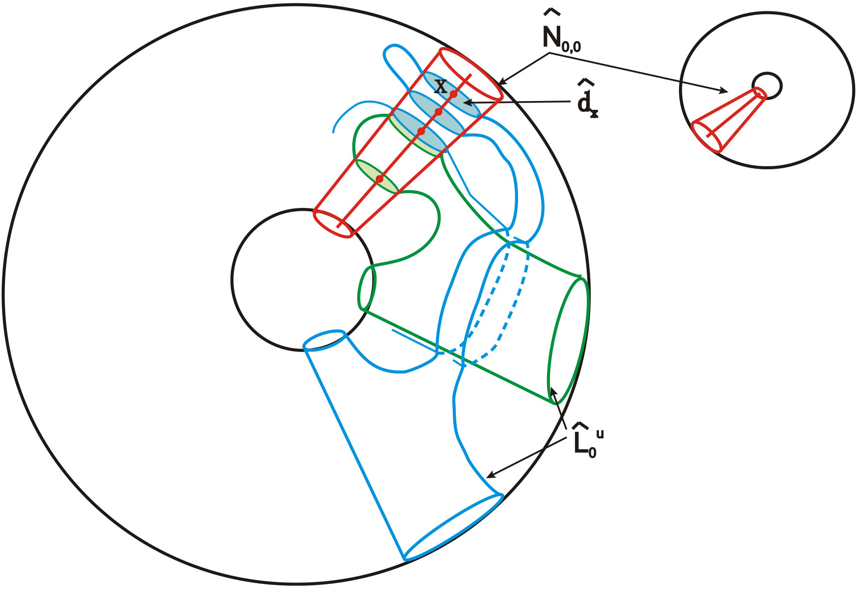 Figure 1
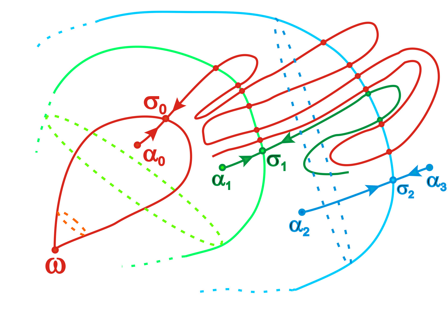 Figure 2
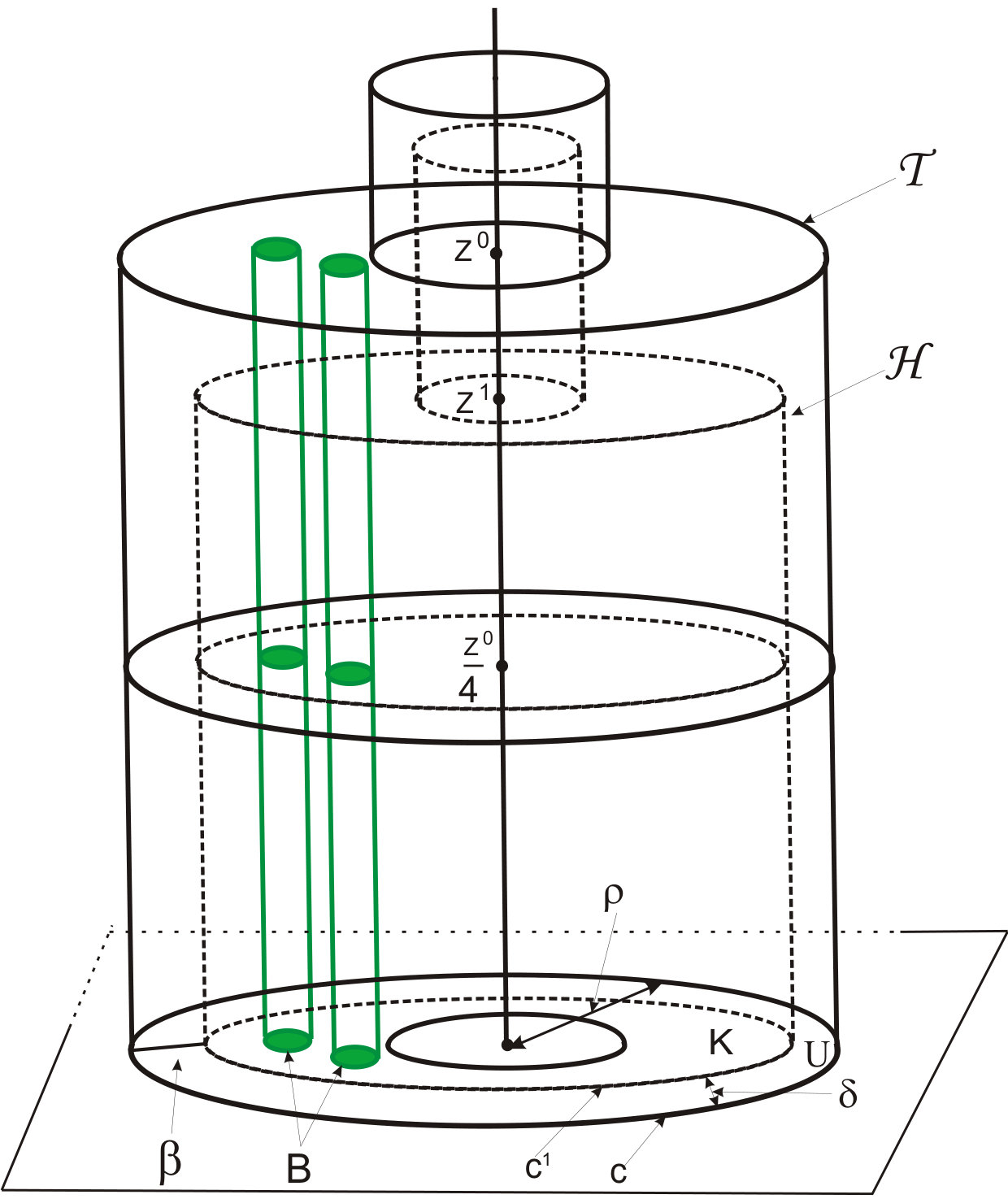 Figure 3
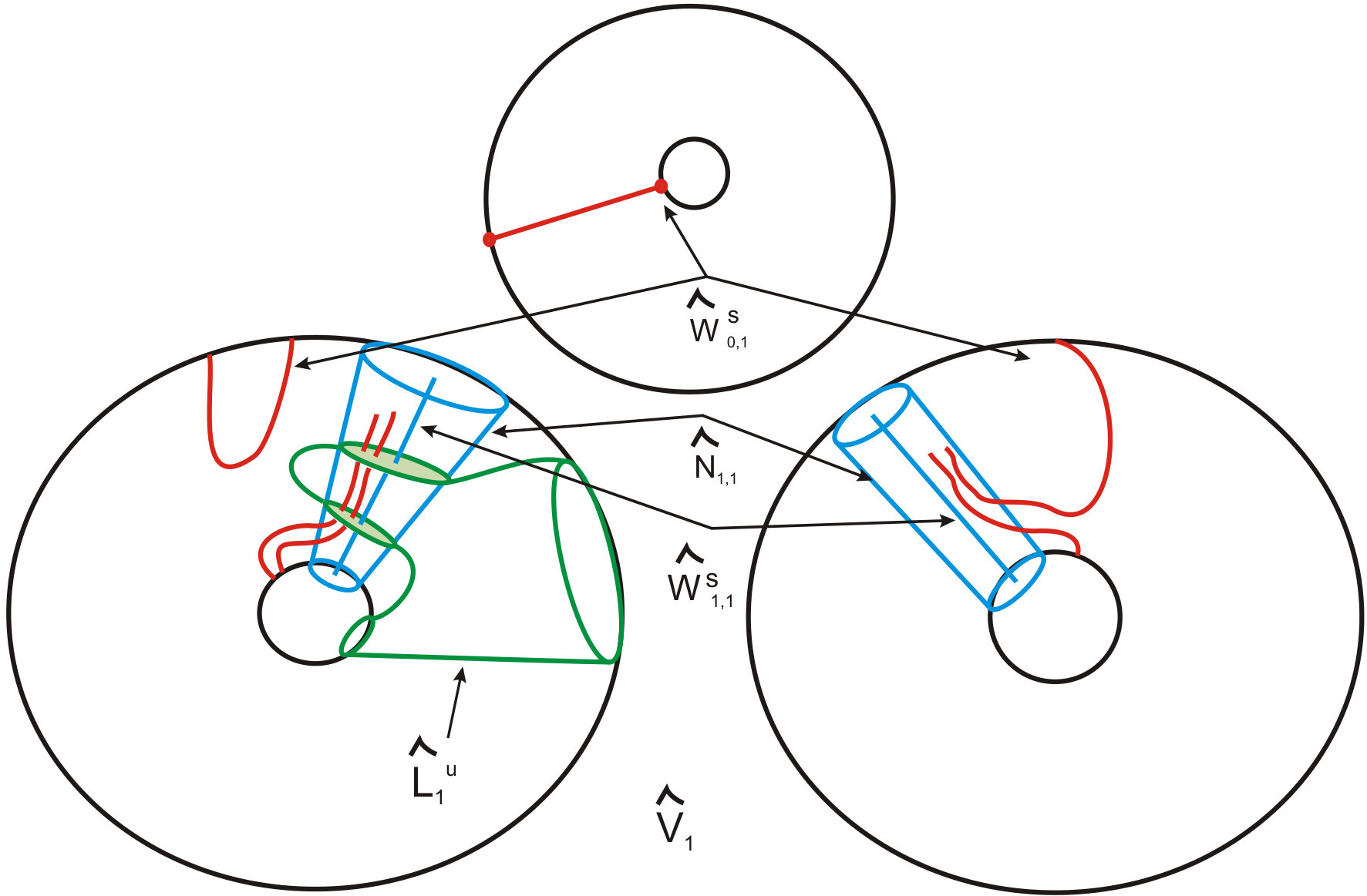 Figure 4
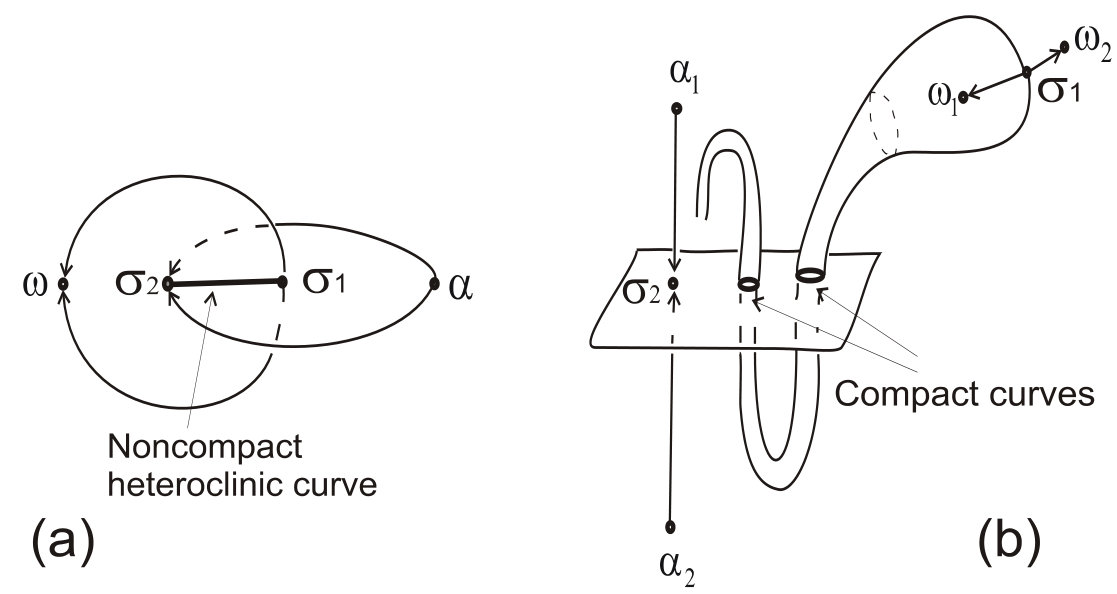 Figure 5
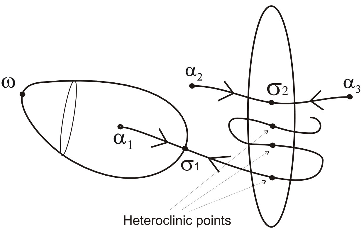 Figure 6
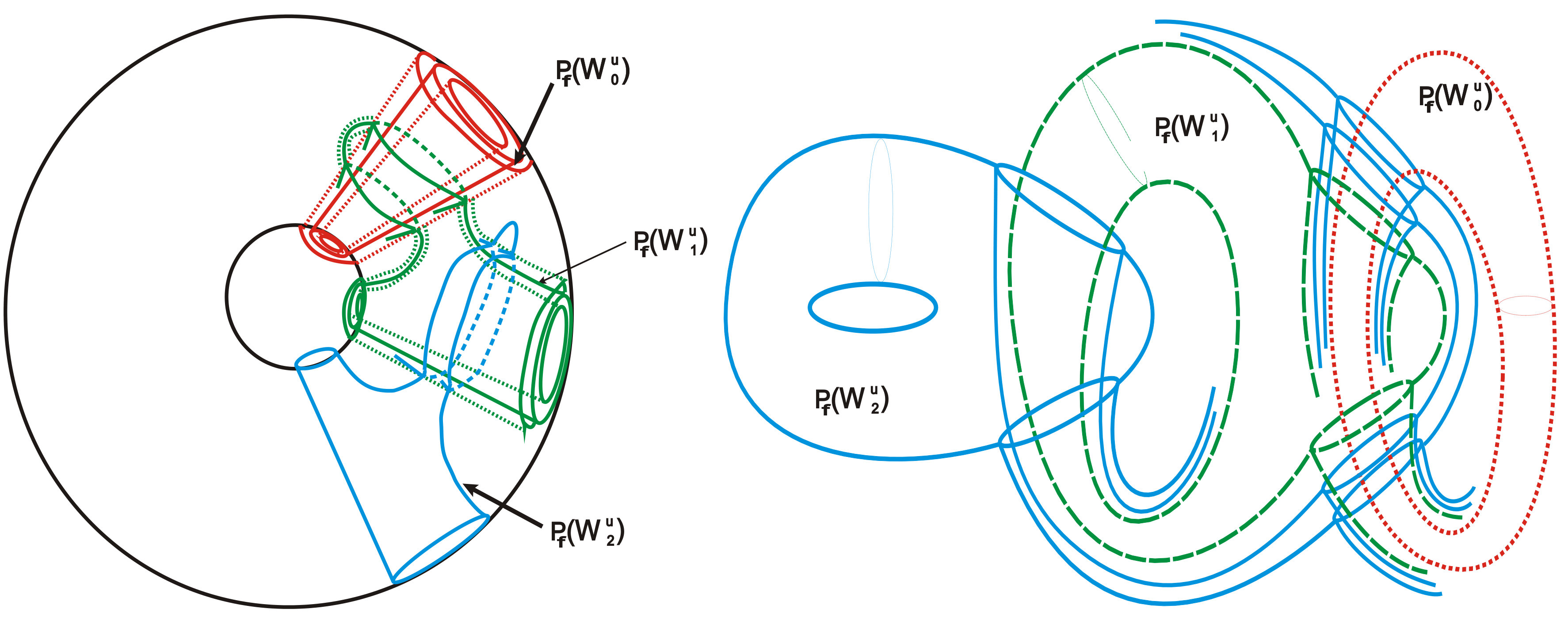 Figure 7