Quantum simulation of molecular spectroscopy in trapped-ion device
Yangchao Shen, Joonsuk Huh, Yao Lu, Junhua Zhang, Kuan Zhang,, Shuaining Zhang, Kihwan Kim

TL;DR
This paper reports the first experimental demonstration of molecular vibrational spectroscopy using a trapped-ion quantum system, showcasing a promising approach for large-scale quantum simulations of complex molecules.
Contribution
It experimentally implements a molecular spectroscopic process in a trapped-ion system using Gaussian transformations, advancing quantum simulation capabilities.
Findings
Successful reconstruction of molecular spectroscopic signals
Implementation of multimode Gaussian transformations via Raman lasers
Paves the way for large-scale quantum molecular simulations
Abstract
Molecules are the most demanding quantum systems to be simulated by quantum computers because of their complexity and the emergent role of quantum nature. The recent theoretical proposal of Huh et al. (Nature Photon., 9, 615 (2015)) showed that a multi-photon network with a Gaussian input state can simulate a molecular spectroscopic process. Here, we report the first experimental demonstration of molecular vibrational spectroscopy of SO with a trapped-ion system. In our realization, the molecular scattering operation is decomposed to a series of elementary quantum optical operations, which are implemented through Raman laser beams, resulting in a multimode Gaussian (Bogoliubov) transformation. The molecular spectroscopic signal is reconstructed from the collective projection measurements on phonon modes of the trapped-ion system. Our experimental demonstration would pave the way…
Click any figure to enlarge with its caption.
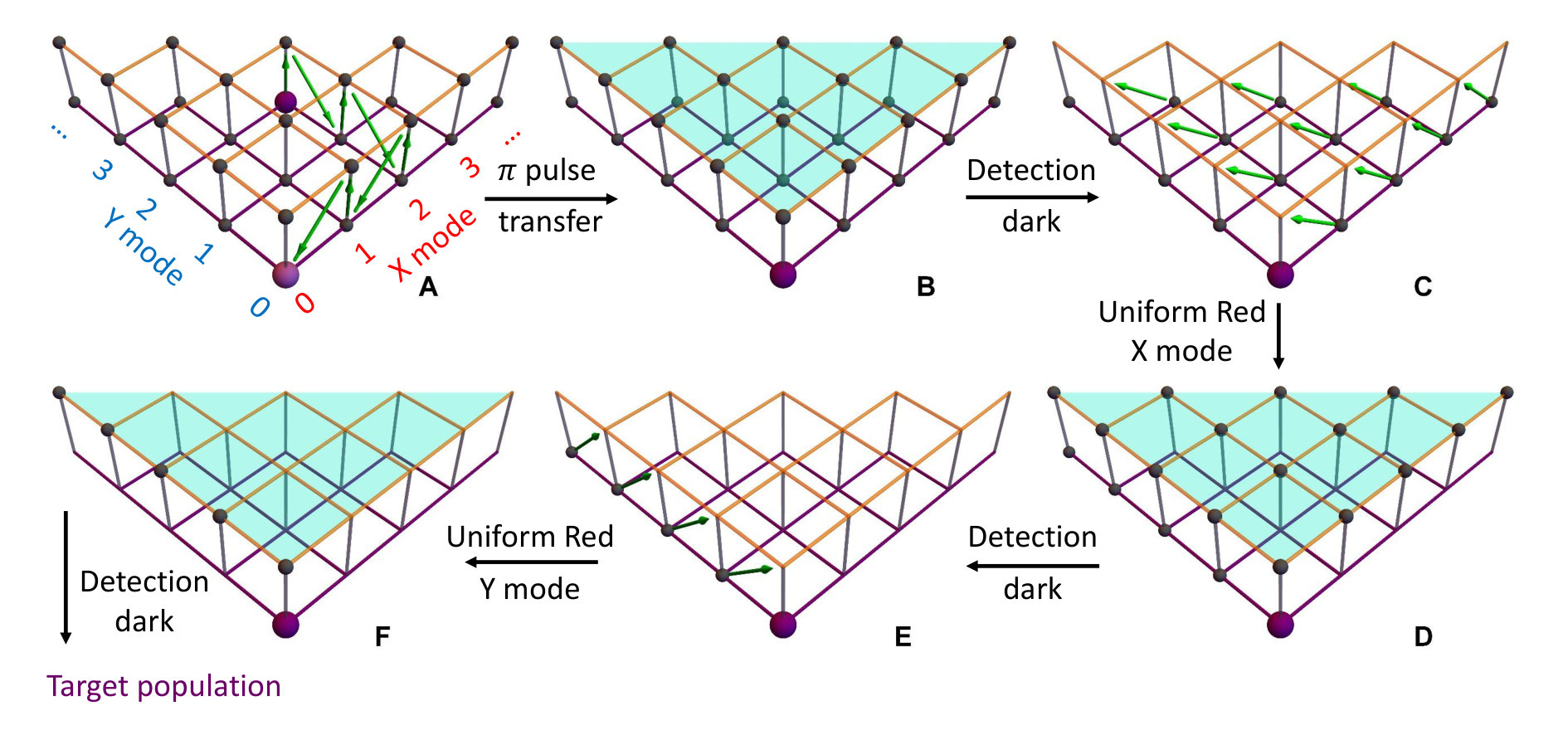 Figure 1
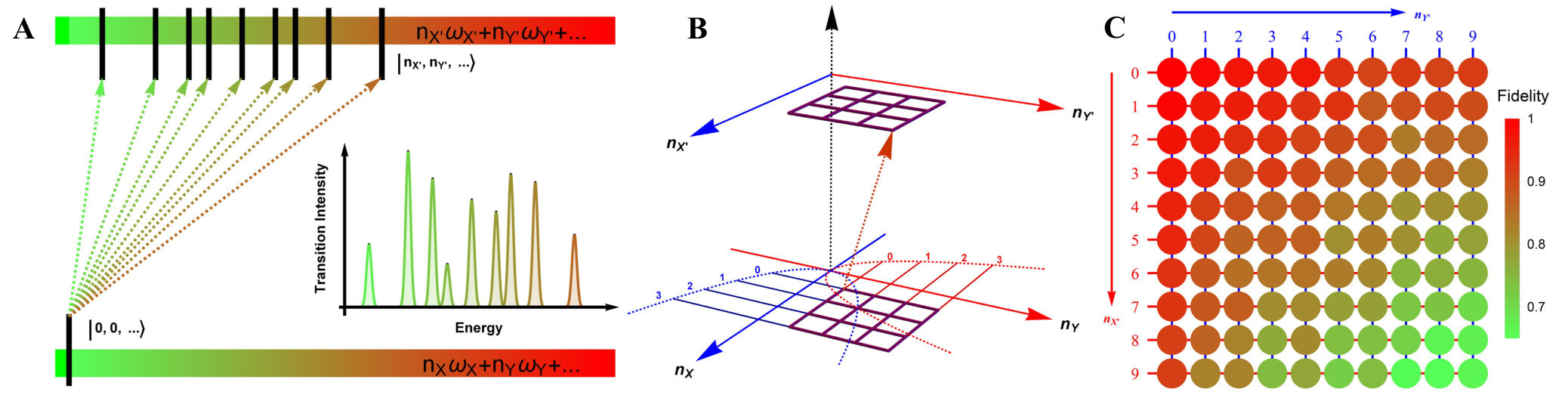 Figure 2
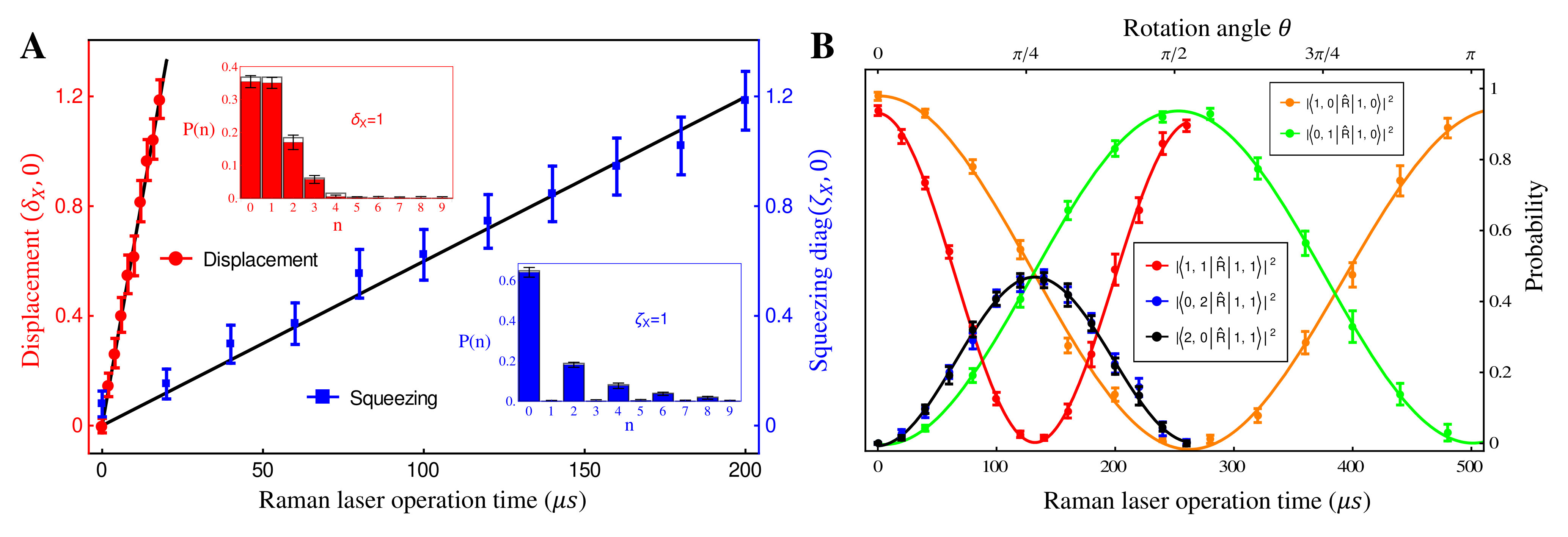 Figure 3
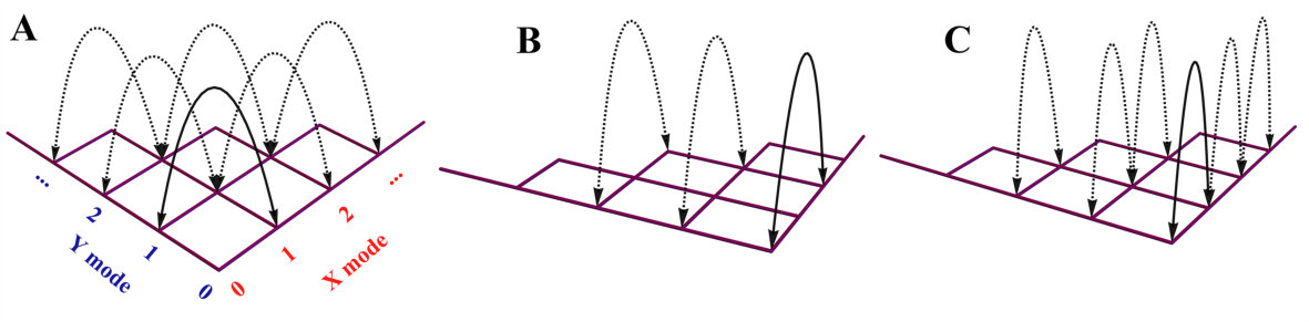 Figure 4
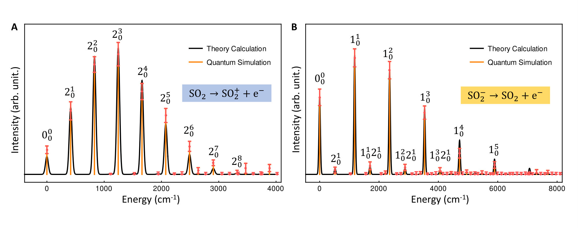 Figure 5
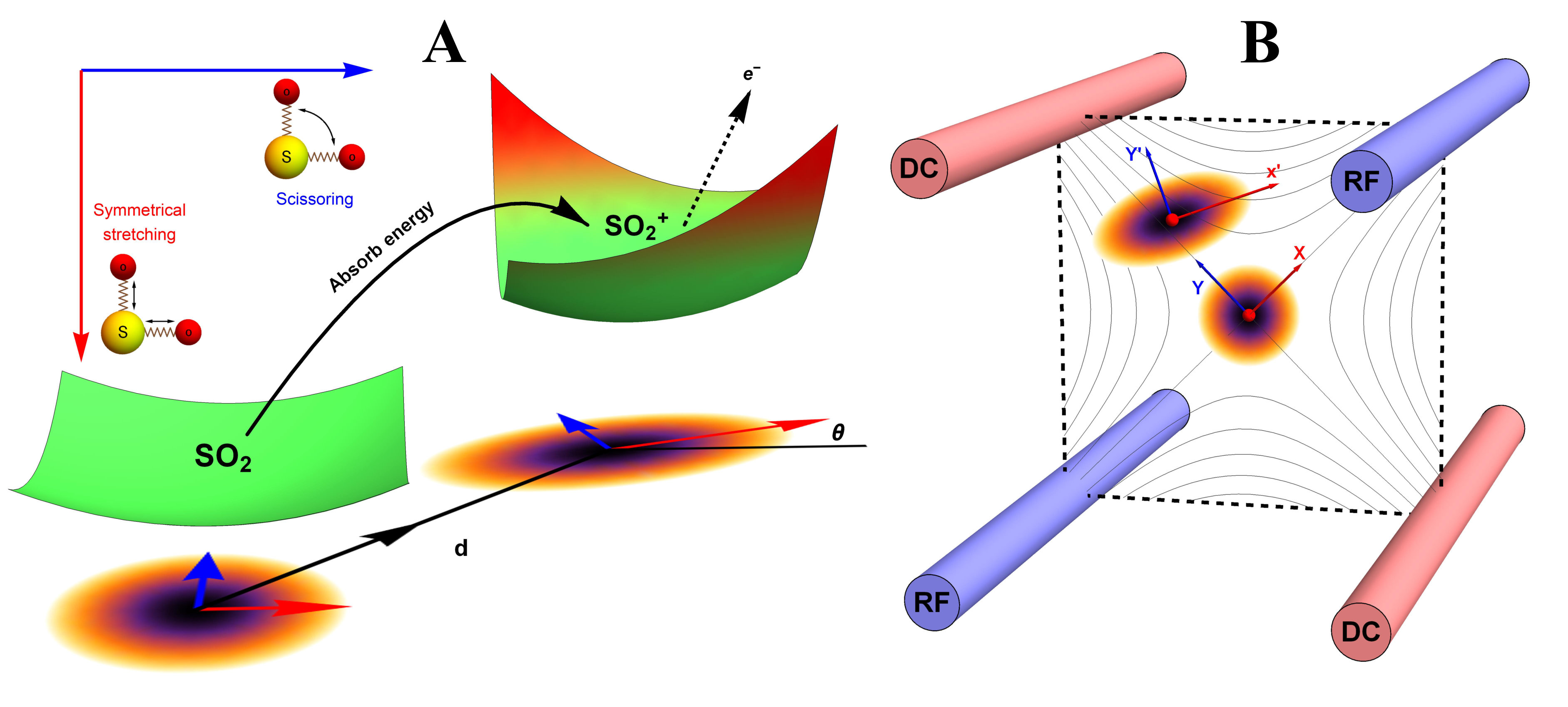 Figure 6
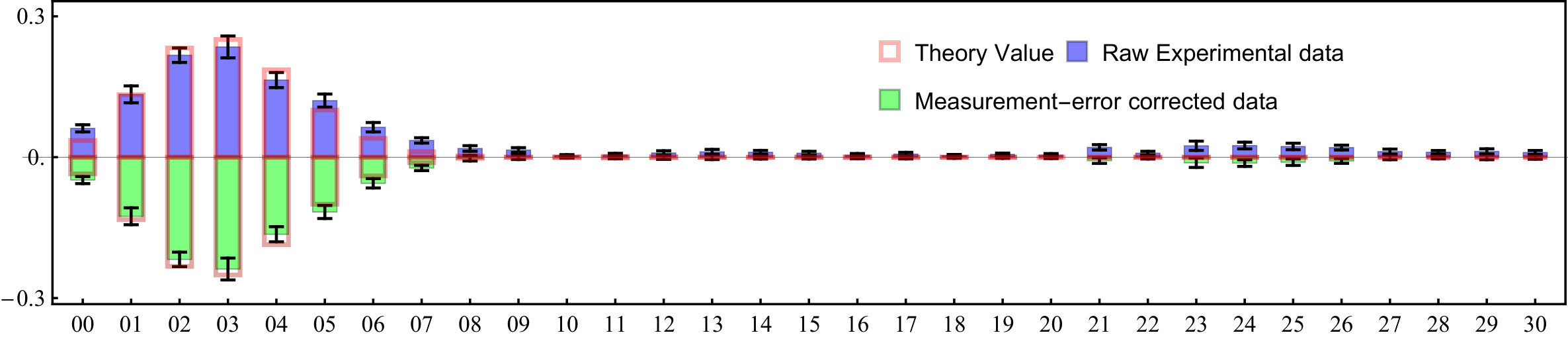 Figure 7
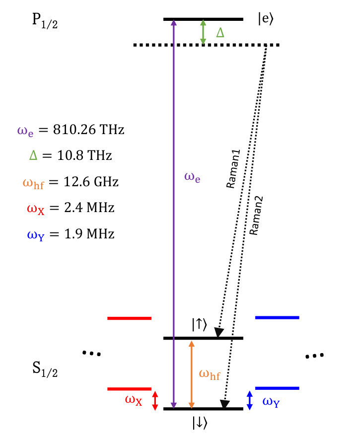 Figure 8
Peer Reviews
No public reviews on file for this paper yet. If you reviewed it on a platform where reviews are public (OpenReview, ICLR, NeurIPS, ICML), you can paste yours below so the community can read it here.
Videos
No videos yet. Explain this paper in a talk, walkthrough, or lecture? Add one.
Quantum simulation of molecular spectroscopy in trapped-ion device
Yangchao Shen1, Joonsuk Huh2∗, Yao Lu1, Junhua Zhang1,
Kuan Zhang1, Shuaining Zhang1 and Kihwan Kim1†
1Center for Quantum Information, IIIS, Tsinghua University, Beijing, P. R. China,
2Department of Chemistry, Sungkyunkwan University, Suwon 440-746, Korea
To whom correspondence should be addressed;
E-mails: ∗[email protected] and †[email protected]
**Molecules are the most demanding quantum systems to be simulated by quantum computers because of their complexity and the emergent role of quantum nature. The recent theoretical proposal of Huh et al. (Nature Photon., 9, 615 (2015)) showed that a multi-photon network with a Gaussian input state can simulate a molecular spectroscopic process. Here, we report the first experimental demonstration of molecular vibrational spectroscopy of SO2 with a trapped-ion system. In our realization, the molecular scattering operation is decomposed to a series of elementary quantum optical operations, which are implemented through Raman laser beams, resulting in a multimode Gaussian (Bogoliubov) transformation. The molecular spectroscopic signal is reconstructed from the collective projection measurements on phonon modes of the trapped-ion system. Our experimental demonstration would pave the way to large-scale molecular quantum simulations, which are classically intractable.
One Sentence Summary: Gaussian boson sampling for photoelectron spectra of sulfur dioxide has been performed using a trapped-ion quantum simulator.**
Boson sampling was originally proposed to simulate a classically intractable multiphoton distribution of indistinguishable photons scattered by beam splitters and phase shifters (?). The successful small-scale experimental implementations (?, ?, ?, ?) of the boson sampling paved the way for quantum simulators regardless of the lack in its obvious practical applications. Alternatively, a modified boson sampling with Gaussian input states, such as thermal and squeezed vacuum states, has been discussed in the computational complexity perspective, classifying that the boson sampling with squeezed states as a classically hard problem (?, ?). Recently, Huh et al. (?, ?) proposed Gaussian boson sampling as a practical application of the boson sampling in connecting the output to the molecular vibronic (vibrational+electronic) spectroscopy. Essentially, boson sampling turned out to be able to not only answer the computational complexity questions but also have a practical application.
The molecular vibronic spectroscopy carries the vibrational transitions between nuclear manifolds belonging to two electronic states of a molecule (?, ?), as shown in Fig. 1(A). Upon the electronic transition, a molecule undergoes structural deformation, vibrational frequency changes and rotation of normal modes; within a harmonic approximation to the electronic potential energy surfaces, these are equivalent to the displacement (), squeezing () and rotation () operations in quantum optics, respectively. The (mass-weighted) normal coordinates of initial () and final () states are related linearly as , where is called the Duschinsky rotation matrix and is a displacement vector of the multidimensional harmonic oscillators in the mass-weighted coordinate, the corresponding dimensionless displacement vector for the quantum optical operation is used later (?). As a result, the molecule performs a multi-mode Bogoliubov transformation (?) between the (vibrational) boson operators of the initial and final electronic states (?, ?). The probability distribution regarding a given molecular vibronic transition frequency () at zero Kelvin, that is, spectrum (Franck-Condon profile), is read as a Fermi’s golden rule for a unitary Gaussian operator (?, ?, ?),
[TABLE]
where , with the -th vibrational frequency () of a molecule in the final electronic state ( belongs to the initial electronic state). The constant off-set frequency , which includes the electronic transition and the zero-point vibrational transition, is set to be zero in this report without losing the generality. and are the initial and final -dimensional Fock states, respectively.
Doktorov et al. (?) decomposed in terms of the elementary quantum optical operators as follows:
[TABLE]
where and are the -mode operators of displacement, squeezing and rotation (?) (see also Supplementary Materials (SM), SM.A.); is a (dimensionless) molecular displacement vector, and are diagnoal matrices of the squeezing parameters, and is a unitary rotation matrix. The actions of the quantum optical operators are defined in Ref. (?). Therefore, the sequential operations of the quantum optical operators in Eq. (2) to the vacuum state and the measurement in Fock basis, as in Eq. (1) (?), can simulate the Franck-Condon profile.
Not only the original boson sampling but also the Gaussian boson sampling for the vibronic spectrum, however, are challenging in an optical system (?, ?, ?, ?) because of the difficulties in preparing the initial states: single Fock states for the original boson sampling and squeezed coherent states for the molecular simulation. Non-optical boson sampling devices, such as trapped-ion (?, ?) and superconducting circuit (?), have been suggested theoretically for the scalable boson sampling machine to overcome the difficulties of the optical implementation in preparing the single photon states. Moreover, these non-optical devices can handle the squeezed states with relative ease. In this report, we present the first quantum simulation of molecular vibronic spectroscopy with a particular example of photoelectron spectroscopy of sulfur dioxide (SO2) (?, ?).
Fig. 1(B) schematically illustrates quantum optical operations of Eq. (2) in the trapped-ion device for the molecular vibronic spectroscopy of SO2. Our trapped-ion simulation is performed using a single ion confined in the 3-dimensional harmonic potential generated by the four-rod trap. The two radial phonon modes (X and Y) of an ion, with the trap frequencies and , map the two vibrational modes of the molecule. After the mapping of the Hilbert space between the real molecule and simulator is established, the molecular spectroscopy is simulated through the following procedure: (i) the ion is first initialized in the motional ground state, (ii) the quantum optical operations in Eq. (2) are then sequentially applied, and (iii) finally, the vibronic spectrum is constructed using the collective projection measurements on the transformed state.
Accordingly, for the first step of the molecular spectroscopy simulation, we prepare the ion in the ground state by the Doppler cooling and the resolved sideband cooling methods (?, ?). Next, we perform the required displacement, squeezing and rotation operations by converting the molecular parameters to the corresponding device parameters. The molecular parameters and can be obtained via conventional quantum chemical calculations with available program packages (e.g., Ref. (?)). See SM.B., for the details of the parameter conversion for SO2.
The quantum optical operations (displacement , squeezing and rotation ) are implemented by the -polarized Raman laser beams from a pico-second pulse laser with a wavelength of 375 nm (see SM.C.). In the trapped-ion experiment, the quantum optical operations with the desired parameters can be performed by controlling the duration and relative phase of the Raman beams. Therefore, the different Raman laser beams with frequencies of , and are assigned for displacement, squeezing and rotation operations, respectively (?, ?). Fig. 2(A) shows the performance of the experimental displacement and squeezing operations, where and are the annihilation and creation operators of bosonic mode X, respectively. The amount of the displacement and the squeezing parameter are controlled by the duration of the corresponding Raman beams with the rates of 0.066 and 0.006 , respectively. We examine the trapped-ion implementation of the rotation operation between modes X and Y with two sets of initial states, as indicated in Fig. 2(B). The rotation angle is also controlled by the duration of the operation with a rate of 0.006 rad . The oscillations in Fig. 2(B) of the initial state (orange and green) are twice slower than those from state (blue, black and red), as expected. We note that at , the near zero probability of originates from the Hong-Ou-Mandel interference (?).
Fig. 3(A) depicts a scheme for reconstructing the spectrum at zero Kelvin from the output measurements of the trapped-ion simulator, the transition intensities from the ground state to the excited states are aligned according to the transition frequencies. Fig. 3(B) illustrates the transition between the two-dimensional Fock spaces resulting from the two-dimensional harmonic oscillators. Finally, We perform the collective quantum-projection measurement of the final state advanced from the measurement scheme of Ref. (?, ?): first, we transfer the population of a target state to the state by a sequence of -pulse transitions. Then, we measure the state population by applying three sequential fluorescence-detections combined with the uniform red sideband technique (see SM.D. for the detailed information). Our quantum projection measurement is limited by the imperfection of the state transfer and the fluorescence-detection efficiency (see SM.E.). We plot the fidelity of the collective projection measurement of state in Fig. 3(C). Based on the fidelity analysis, We perform measurement-error corrections for the experimental raw data (see SM.E. for the detailed information).
Furthermore, We simulate the photoelectron spectroscopies of SO2 and SO, in which a single electron is removed from the molecule during the photon absorption process, with our trapped-ion quantum simulator. Owing to the symmetry of the molecules, we use only two vibrational modes of sulfur dioxide, which show mixing of the vibration modes with respect to the final vibrational coordinates (?), in our quantum simulation for the molecular spectra; the remaining vibrational mode does not contribute to the overall spectral shape because SO2 does not deform along the remaining (non-totally-symmetric) vibrational mode during the vibronic transition.
Fig. 4 presents the photoelectron spectra, SOSO and SOSO2 obtained from our trapped-ion quantum simulation, this is compared with the theoretical classical calculations. Fig. 4 shows good agreement between the theory calculations and the trapped-ion simulations of the two photoelectron processes of sulfur dioxide, the required molecular parameters are described in the figure caption. In Fig. 4(A), the photoelectron spectrum of SO2 is dominated by transitions due to the significant large displacement along the second mode: . The photoelectron spectrum of SO in Fig. 4(B) shows tiny combination bands of the first and second modes regardless of the dominant contribution of the first mode (). We note that the observation of the tiny band combinations indicates reliable performance of the trapped-ion simulation.
As the first demonstration of quantum simulation for the molecular vibronic spectroscopy, our trapped-ion device shows an excellent performance at a small-scale after the error-correction scheme in SM.E. In the near future, we expect the many modes implementation for a large-scale molecular simulation, where the multi-modes can be mapped to the local vibrational modes or collective normal modes of many ions in a single trap. The demonstrated quantum optical operations through a single ion will be directly applied for the large-scale simulation. This would be useful in concluding the quantum supremacy of boson sampling with the Gaussian states. The molecular simulations in trapped-ion devices and the real molecular spectroscopic signals can be compared as a certification protocol for large-scale Gaussian boson sampling, which cannot be verified classically because of the #P-hardness (?, ?, ?).
References and Notes
S. Aaronson, A. Arkhipov, Proceedings of the 43rd annual ACM symposium on Theory of computing - STOC ’11 p. 333 (2011).
- 2.
J. B. Spring, et al., Science 339, 798 (2013).
- 3.
M. A. Broome, et al., Science 339, 794 (2013).
- 4.
A. Crespi, et al., Nature Photon. 7, 545 (2013).
- 5.
M. Tillmann, et al., Nature Photon. 7, 540 (2013).
- 6.
A. P. Lund, et al., Phys. Rev. Lett. 113, 100502 (2014).
- 7.
S. Rahimi-Keshari, A. P. Lund, T. C. Ralph, Phys. Rev. Lett. 114, 060501 (2015).
- 8.
J. Huh, G. G. Guerreschi, B. Peropadre, J. R. McClean, A. Aspuru-Guzik, Nature Photon. 9, 615 (2015).
- 9.
J. Huh, M.-H. Yung, arXiv:1608.03731 (2016).
- 10.
H.-C. Jankowiak, J. L. Stuber, R. Berger, J. Chem. Phys. 127, 234101 (2007).
- 11.
S. L. Braunstein, Phys. Rev. A 71, 1 (2005).
- 12.
E. V. Doktorov, I. A. Malkin, V. I. Man’ko, J. Mol. Spectrosc. 64, 302 (1977).
- 13.
X. Ma, W. Rhodes, Phys. Rev. A 41, 4625 (1990).
- 14.
H. K. Lau, D. F. V. James, Phys. Rev. A 85, 059905 (2012).
- 15.
C. Shen, Z. Zhang, L. M. Duan, Phys. Rev. Lett. 112, 1 (2014).
- 16.
B. Peropadre, G. G. Guerreschi, J. Huh, A. Aspuru-Guzik, Phys. Rev. Lett. 117, 140505 (2016).
- 17.
M. Nimlos, G. Ellison, J. Phys. Chem. 90, 2574 (1986).
- 18.
C.-L. Lee, S.-H. Yang, S.-Y. Kuo, J.-L. Chang, J. Mol. Spectros. 256, 279 (2009).
- 19.
C. Monroe, D. M. Meekhof, B. E. King, W. M. Itano, D. J. Wineland, Phys. Rev. Lett. 75, 4714 (1995).
- 20.
C. Roos, et al., Phys. Rev. Lett. 83, 4713 (1999).
- 21.
M. J. Frisch, et al., Gaussian˜16 Revision A.03 (2016). Gaussian Inc. Wallingford CT.
- 22.
D. M. Meekhof, C. Monroe, B. E. King, W. M. Itano, D. J. Wineland, Phys. Rev. Lett. 76, 1796 (1996).
- 23.
K. Toyoda, R. Hiji, A. Noguchi, S. Urabe, Nature 527, 74 (2015).
- 24.
M. Um, et al., Nat. Commun. 7, 11410 (2016).
- 25.
J. Zhang, et al., arXiv:1611.08700 (2016).
Acknowledgments:
This work was supported by the National Key Research and Development Program of China under Grants No. 2016YFA0301900 (No. 2016YFA0301901), the National Natural Science Foundation of China Grant 11374178 and 11574002. JH acknowledges the supports by Basic Science Research Program through the National Research Foundation of Korea (NRF) funded by the Ministry of Education, Science and Technology (NRF-2015R1A6A3A04059773), the ICT R&D program of MSIP/IITP [1711028311] and Mueunjae Institute for Chemistry (MIC) postdoctoral fellowship.
Supplementary Materials: Quantum simulation of molecular spectroscopy in trapped-ion device
Yangchao Shen1, Joonsuk Huh2∗, Yao Lu1, Junhua Zhang1,
Kuan Zhang1, Shuaining Zhang1 and Kihwan Kim1†
1Center for Quantum Information, IIIS, Tsinghua University, Beijing, P. R. China,
2Department of Chemistry, Sungkyunkwan University, Suwon 440-746, Korea
To whom correspondence should be addressed;
E-mails: ∗[email protected] and †[email protected]
A. Quantum optical operators
We define, herein, the quantum optical operators we have used in our work. and are -dimensional column vectors for the bosonic annihilation and creation operators, respectively. That is,
[TABLE]
where .
The -mode displacement operator is defined as below with the displacement vector ,
[TABLE]
The -mode squeezing operator is defined as below with the squeezing parameter matrix .
[TABLE]
The -mode rotation operator is defined as below with a unitary matrix ,
[TABLE]
B. Experimental parameters for quantum optical operations
We present, here, the parameters used in the trapped-ion device for the quantum optical operations. The displacement operator with two modes is rewritten as follows,
[TABLE]
As seen in Eq. S5, the displacement operations of the X and Y modes can be implemented independently.
The squeezing operator with the two mode parameter can be rewritten as follows,
[TABLE]
In the trapped-ion experiment, the squeezing operations are limited to the range of in Eq. S6. Since involves the squeezing and inverse squeezing operations, we can freely rescale the squeezing parameters with a single arbitrary constant: we rescale the squeezing parameters by a factor of 1/25, and (\zeta_{\rm X}^{\prime},\zeta_{\rm Y}^{\prime})=(\ln(\sqrt{\omega_{1}^{\prime}}/25),$$\ln(\sqrt{\omega_{2}^{\prime}}/25)). The rescaling parameter is canceled after the two squeezing operations.
The two mode rotation operation can be written simply with a rotation angle ,
[TABLE]
where becomes the unitary rotation matrix. The rotation angle is controlled by Raman laser beams in the trapped-ion simulation.
C. Quantum optical operations in trapped-ion system
We implement the quantum optical operations (, and ) via controlling Raman laser beams. Figure S1 shows the energy diagram of a trapped . The two levels in hyperfine structure of manifold is usually used to realize a qubit, which are denoted as and . The red (mode X) and blue (mode Y) lines stand for the motional degrees of freedom. The Raman process is implemented via the virtual energy level, which is detuned from level, . Our quantum optical operations can be implemented by applying different frequencies of Raman laser beams.
To show how we can implement the quantum optical operations with the Raman laser beams, we start from a light-matter Hamiltonian. Based on the energy level diagram of Figure S1, the Hamiltonian for the whole system (atom and laser) can be written as,
[TABLE]
where with the condition of and for the contour-propagating geometry of Raman laser beams. represents the strength of the dipole coupling between and . Here stand for the Raman beam.
After introducing the interaction picture to the Hamiltonian with respect to the system part, ; and by setting two Raman laser beam frequencies as , which is represented by the configuration shown in Fig. S2(A) ; finally, by using rotating wave and Lamb-Dicke approximation together with the experimental conditions of , we arrive at the Hamiltonian for the rotation operation as,
[TABLE]
which leads to the rotation
[TABLE]
Here , is the relative phase between two Raman beams, and , are the Lamb-Dicke parameter for the Raman process. In the experiment, we set rad .
Similarly, we can perform the squeezing operation of single motional mode (here, mode X as an example) by setting two Raman laser frequencies as , which leads the configuration shown in Fig. S2(B),
[TABLE]
where . In the experiment, we set .
The displacement operation of single mode (here, mode X as an example) by setting two Raman laser frequencies , which leads the configuration shown in Fig. S2(C),
[TABLE]
where . In the experiment, we set .
D. Method for collective projection measurements
We explain in this section the pulse sequence for the detection of population in an arbitrary phonon state , where we indicate the internal qubit state ( or ) of the phonon state ().
The first step is to transfer the population in the target state to : it is performed by applying a sequence of -pulse transitions, as shown in Fig. S3(A), i.e., with the following steps,
[TABLE]
The second step is to obtain the population in by using the sequence as shown in Fig. S3(B-F).
(B): Apply the fluorescence detection and record the event of detecting photons or no photons.
(C): Apply a uniform red-transition on mode X, which transfers all the states of to state.
(D): Apply the fluorescence detection and record the event of detecting photons or no photons.
(E): Apply a uniform red-transition on Y mode, which transfers all the states of to state.
(F): Apply the fluorescence detection and record the event of detecting photons or no photons.
In the above multiple-detection stages, there are four situations for the recorded data
[TABLE]
Here, means detecting no photons, means detecting photons, stands for both situations. Typically, we repeat the experiments for 2000 times to get the probability for each case noted as . The population of the target state is the probability of case .
Within the above collective projection measurements, Fig. 3(C) shows the experimentally measured result for the fidelity of the detection sequence of an arbitrary state , noted as . The infidelity mainly comes from the imperfection of -pulse and uniform red-transition on X and Y mode.
E. Measurement-error corrections for the experimental raw data
We mainly consider two error sources to correct the experimental raw data: i) the inefficiency of fluorescence detection of internal states; ii) the infidelity of the collective projection measurement discussed in section D.
Our fluorescence detection can distinguish the internal states and with the corresponding detection fidelities are state and for state, respectively. To correct this inefficiency, we use the value of , which is obtained by 1-(). The real population () of detecting photons scattered from the state is not exactly same to the measured population (). The relation between them is given as , thus
[TABLE]
For the correction of the second part, as discussed in the section C, we have to include the fidelity .
In order to correct the raw experimental data, we consider these two imperfections. For the experiment raw data, our corrected data is written accordingly as,
[TABLE]
Figure S4 compares the raw experimental data and corrected data for the photoelectron spectroscopy of SO2.
The reference list from the paper itself. Each links out to its DOI / PubMed record.
- 11. S. Aaronson, A. Arkhipov, Proceedings of the 43rd annual ACM symposium on Theory of computing - STOC ’11 p. 333 (2011).
- 22. J. B. Spring, et al. , Science 339 , 798 (2013).
- 33. M. A. Broome, et al. , Science 339 , 794 (2013).
- 44. A. Crespi, et al. , Nature Photon. 7 , 545 (2013).
- 55. M. Tillmann, et al. , Nature Photon. 7 , 540 (2013).
- 66. A. P. Lund, et al. , Phys. Rev. Lett. 113 , 100502 (2014).
- 77. S. Rahimi-Keshari, A. P. Lund, T. C. Ralph, Phys. Rev. Lett. 114 , 060501 (2015).
- 88. J. Huh, G. G. Guerreschi, B. Peropadre, J. R. Mc Clean, A. Aspuru-Guzik, Nature Photon. 9 , 615 (2015).