Low-resolution simulations of vesicle suspensions in 2D
Gokberk Kabacaoglu, Bryan Quaife, George Biros

TL;DR
This paper develops a low-resolution simulation scheme for vesicle suspensions that is faster and maintains accuracy, by systematically integrating empirical fixes to improve stability and physical fidelity.
Contribution
It introduces a systematic low-resolution correction algorithm (LRCA) for vesicle suspension simulations, enhancing efficiency and accuracy over previous methods.
Findings
LRCA enables 10x to 100x faster simulations.
Low-resolution simulations remain statistically accurate.
The scheme effectively handles dense suspensions and vesicle interactions.
Abstract
Vesicle suspensions appear in many biological and industrial applications. These suspensions are characterized by rich and complex dynamics of vesicles due to their interaction with the bulk fluid, and their large deformations and nonlinear elastic properties. Many existing state-of-the-art numerical schemes can resolve such complex vesicle flows. However, even when using provably optimal algorithms, these simulations can be computationally expensive, especially for suspensions with a large number of vesicles. In this paper, we investigate the effect of a number of algorithmic empirical fixes in an attempt to make low-resolution simulations more stable and more predictive. Based on our empirical studies for a number of flow configurations, we propose a scheme that attempts to integrate these fixes in a systematic way. This low-resolution scheme is an extension of our previous work…
Click any figure to enlarge with its caption.
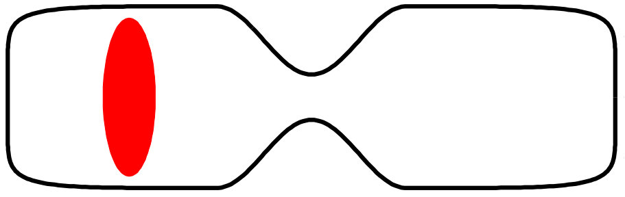 Figure 1
 Figure 2
 Figure 3
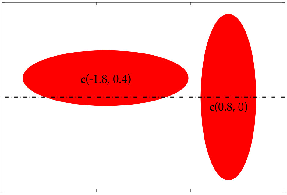 Figure 4
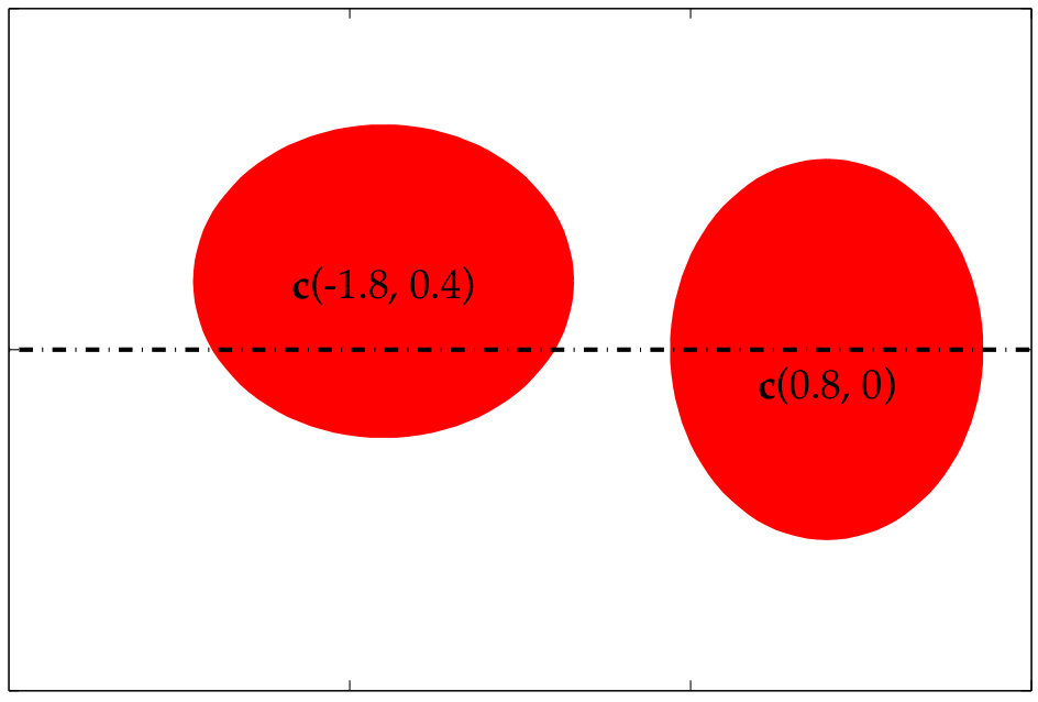 Figure 5
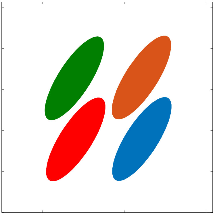 Figure 6
 Figure 7
 Figure 8
 Figure 9
 Figure 10
 Figure 11
 Figure 12
 Figure 13
 Figure 14
 Figure 15
 Figure 16
 Figure 17
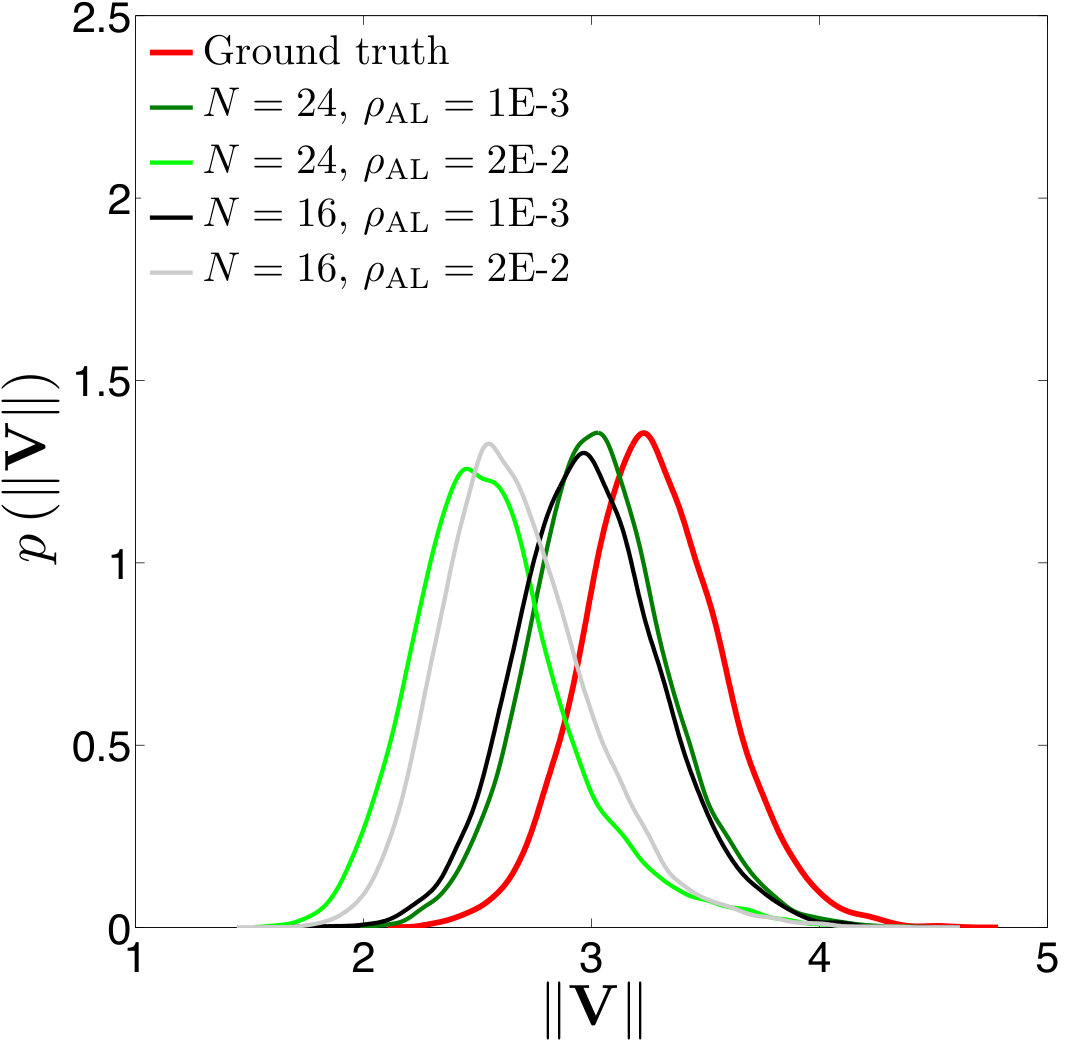 Figure 18
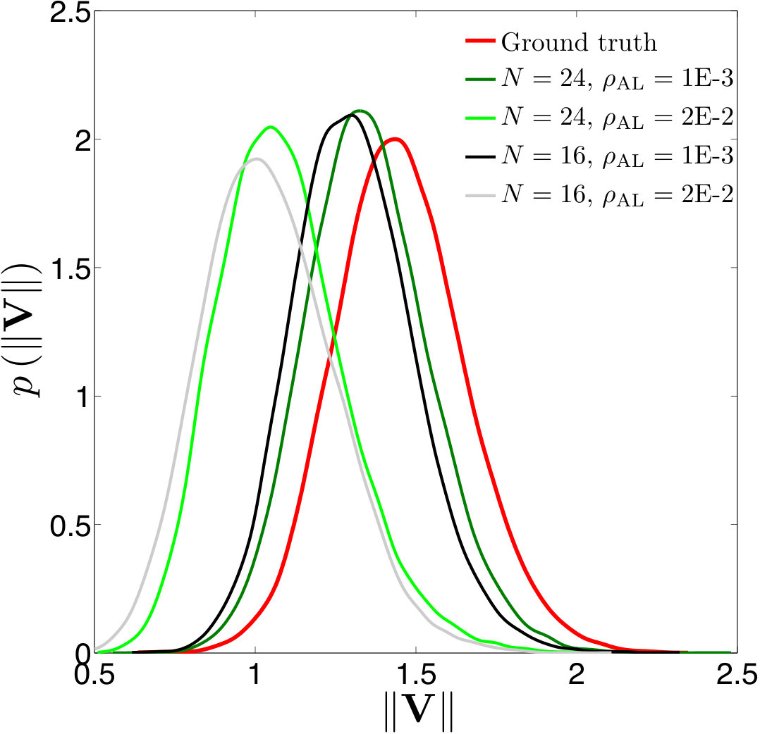 Figure 19
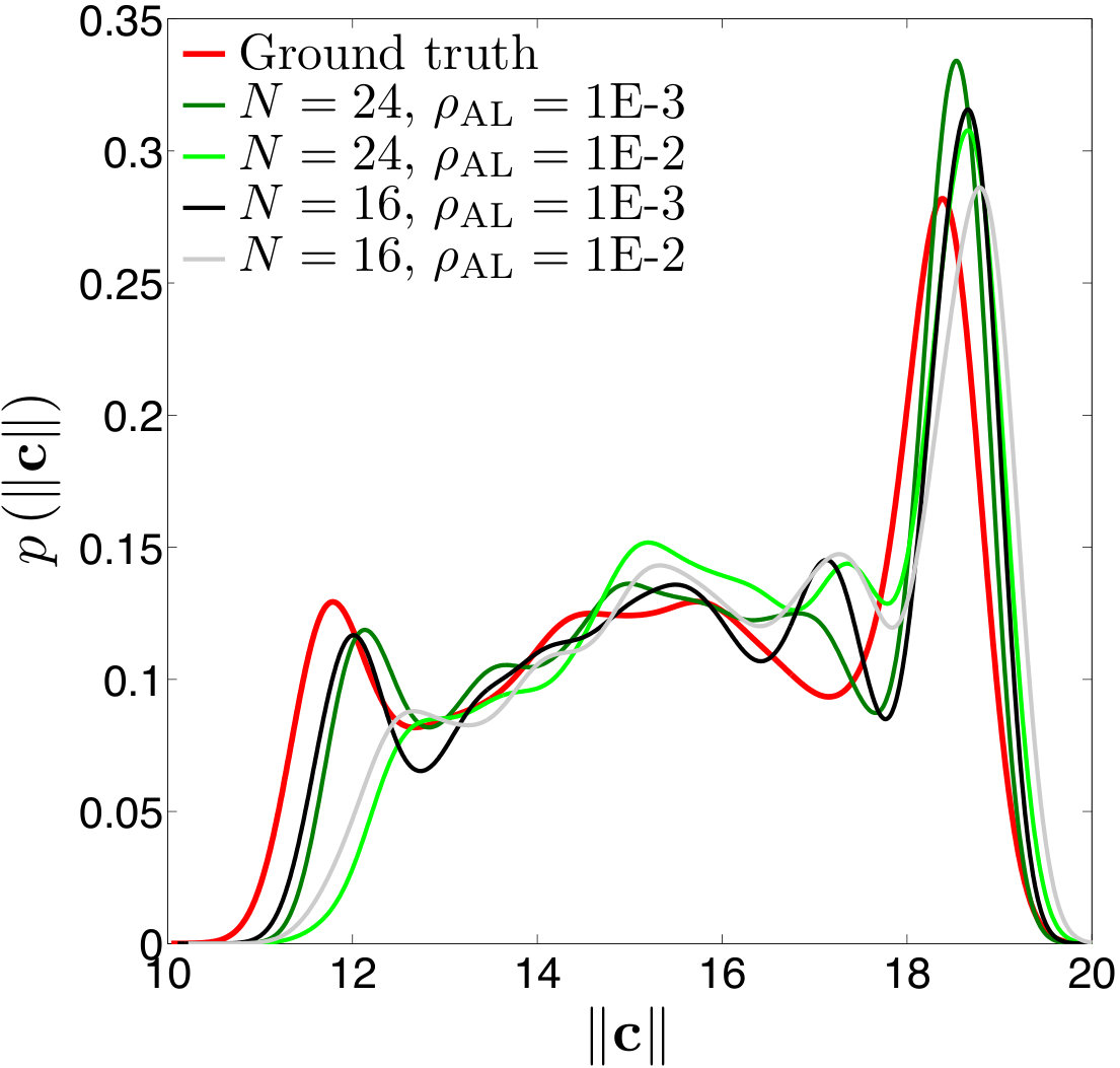 Figure 20
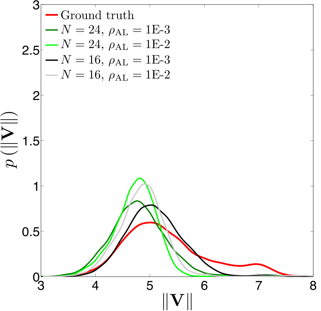 Figure 21
 Figure 22
 Figure 23
 Figure 24
 Figure 25
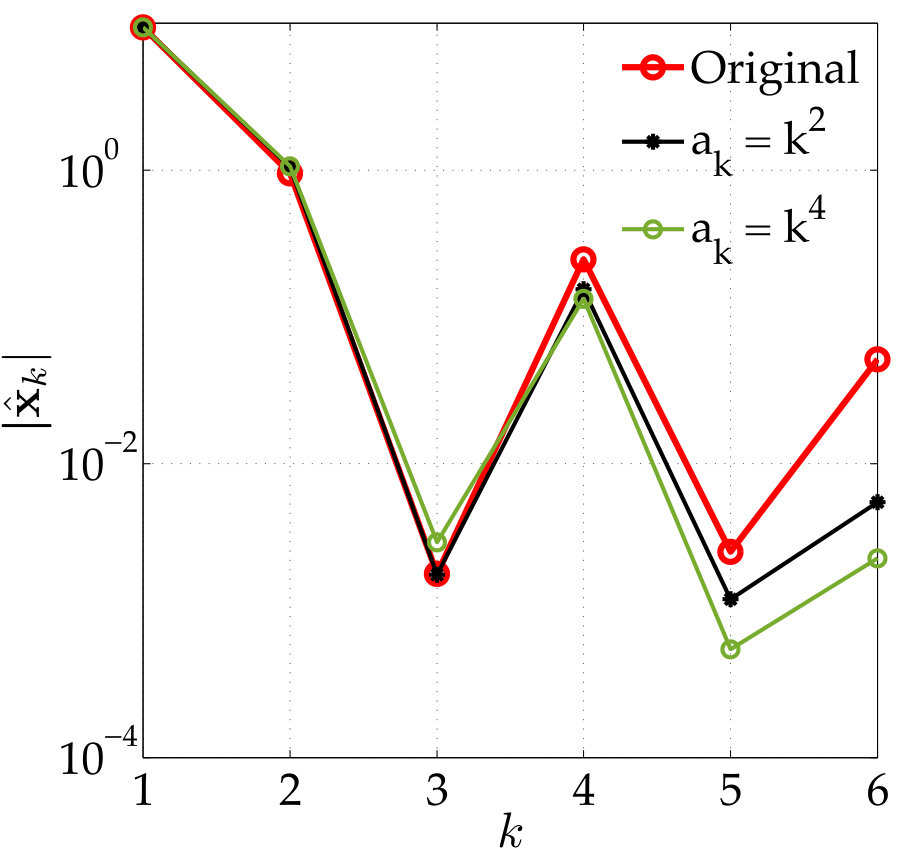 Figure 26
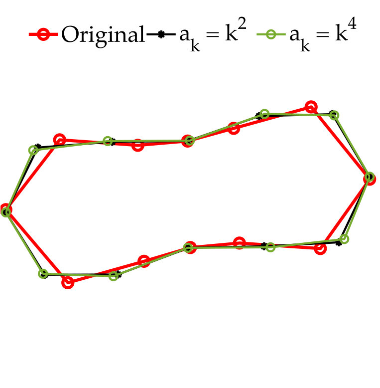 Figure 27
 Figure 28
 Figure 29
 Figure 30
 Figure 31
 Figure 32
 Figure 33
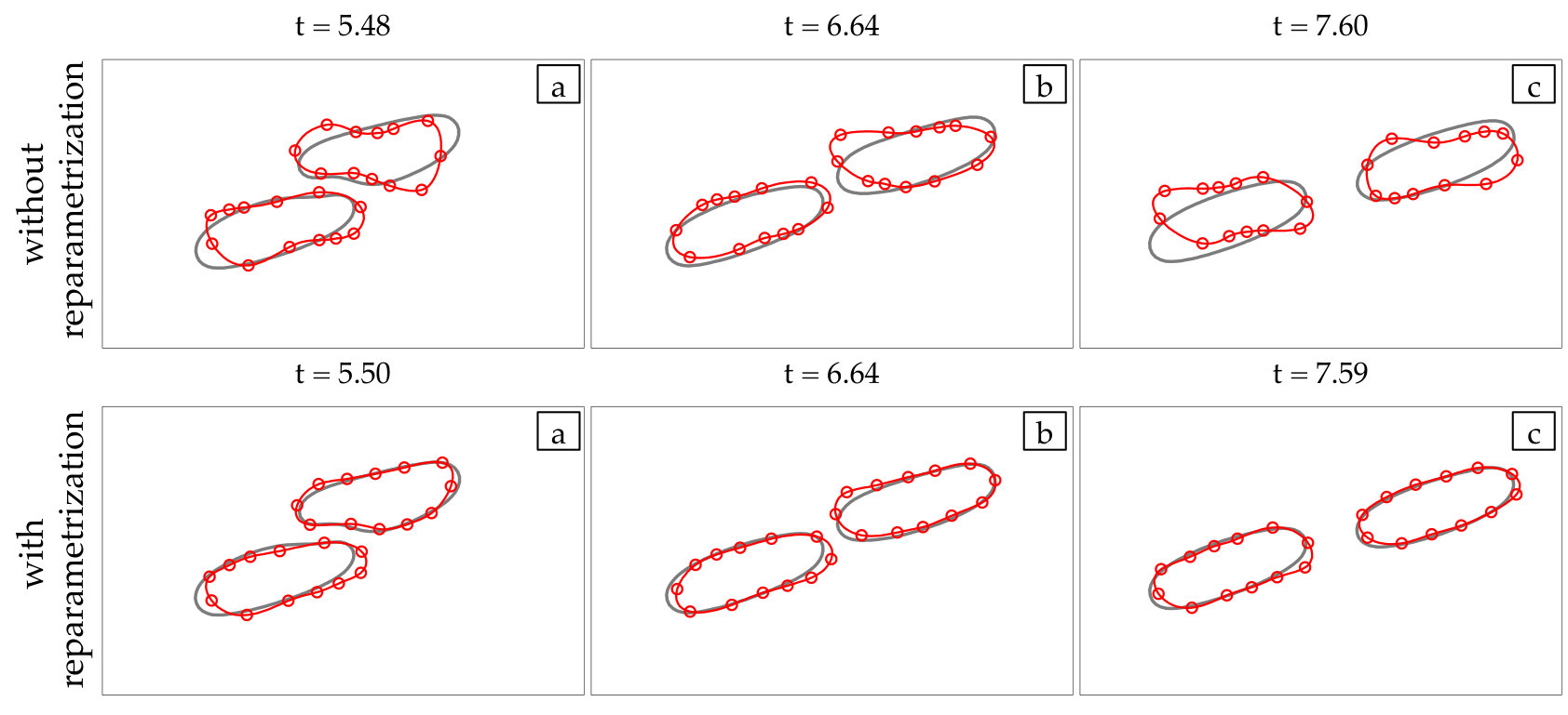 Figure 34
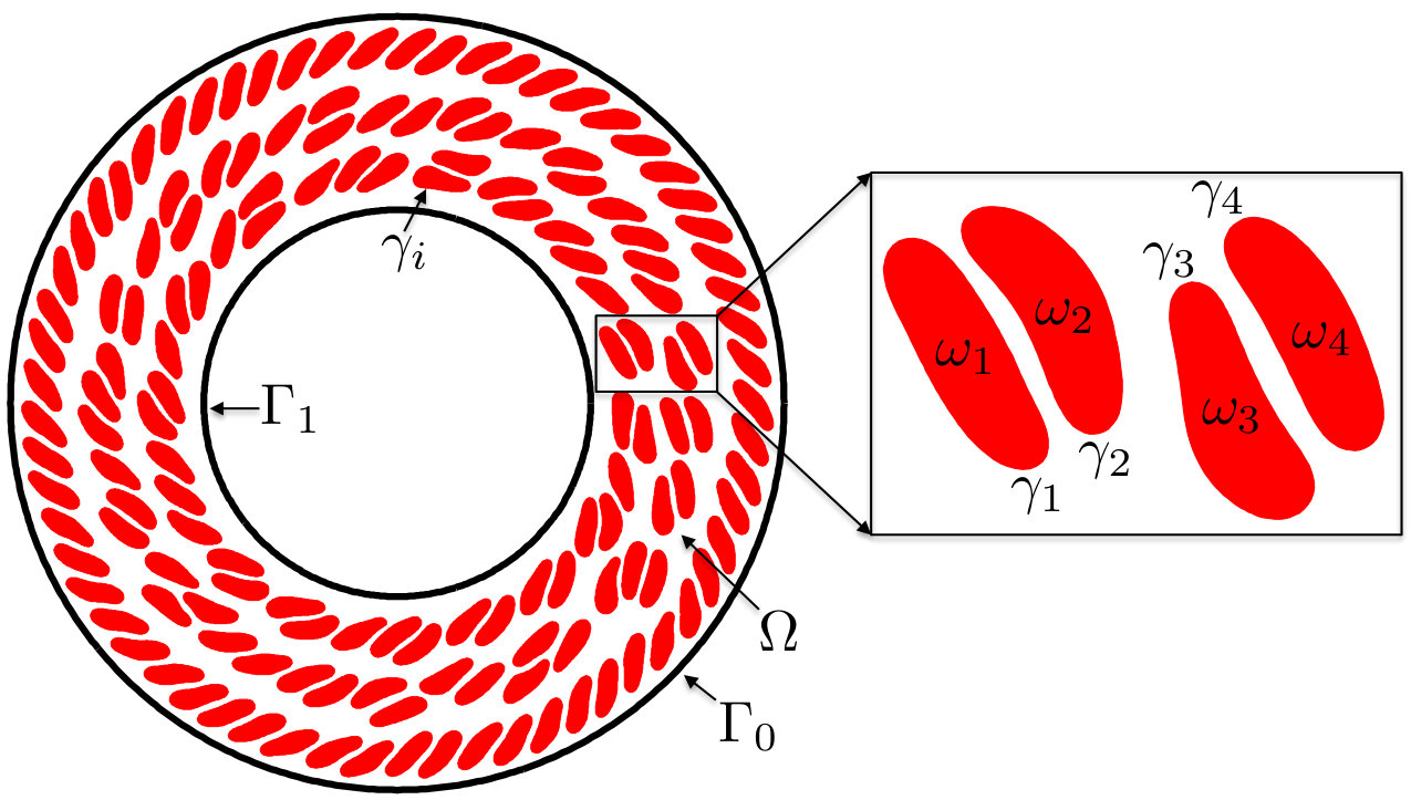 Figure 35
 Figure 36
 Figure 37
 Figure 38
| Symbol | Definition | Value |
|---|---|---|
| Tolerance for errors in area-length | [1E-4, 1E-1] | |
| Tolerance that must be reached for time step to be increased | ||
| Maximum factor of increment in time step size | ||
| Minimum factor of decrement in time step size | ||
| Tolerance for using the asymptotic assumption to increase time step size | ||
| Tolerance for using the asymptotic assumption to decrease time step size | ||
| Maximum time step size |
| LRCA | Original | |||||||||
| Accepts | Rejects | Time (sec) | Accepts | Rejects | Time (sec) | |||||
| 12 | 1E-2 | 1.2E-1 | 4.2E-2 | 94 | 4 | 64 | 2.5E-1 | 128 | 10 | 58 |
| 16 | 1E-3 | 3.7E-2 | 4.7E-2 | 310 | 7 | 193 | 2.0E-1 | 345 | 14 | 132 |
| 24 | 1E-4 | 4.1E-2 | 1.5E-2 | 998 | 11 | 826 | 4.1E-2 | 1026 | 14 | 400 |
| 32 | 1E-5 | 2.8E-2 | 3156 | 15 | 1930 | 9.1E-3 | 3174 | 15 | 808 | |
| 12 | 1E-2 | 1.2E-1 | 3.3E-2 | 94 | 4 | 64 | 2.5E-1 | 128 | 10 | 58 |
| 12 | 1E-3 | 8.0E-2 | 6.8E-2 | 354 | 10 | 348 | 8.4E-2 | 761 | 10 | 335 |
| 12 | 1E-4 | 1.5E-2 | 1165 | 15 | 1150 | 1.0E-2 | 5226 | 16 | 1880 | |
| 16 | 1E-3 | 3.7E-2 | 3.5E-2 | 310 | 7 | 193 | 2.0E-1 | 345 | 14 | 132 |
| 16 | 1E-4 | 2.6E-2 | 955 | 5 | 921 | 1.9E-1 | 2086 | 21 | 889 | |
| LRCA | Original | |||||||||
| Accepts | Rejects | Time (sec) | Accepts | Rejects | Time (sec) | |||||
| 12 | 1E-2 | 5.3E-1 | 1.3E-1 | 110 | 2 | 57 | 5.5E-1 | 110 | 3 | 38 |
| 16 | 1E-3 | 3.4E-1 | 2.6E-1 | 373 | 3 | 199 | 1.1E-1 | 343 | 6 | 134 |
| 24 | 1E-4 | 6.5E-2 | 4.5E-2 | 1192 | 9 | 699 | 1.5E-2 | 1191 | 9 | 446 |
| 32 | 1E-5 | 1.8E-2 | 3766 | 13 | 2300 | 4.8E-3 | 3767 | 13 | 862 | |
| 12 | 1E-2 | 5.3E-1 | 1.9E-1 | 110 | 2 | 57 | 5.5E-1 | 110 | 3 | 38 |
| 12 | 1E-3 | 2.8E-1 | 3.4E-1 | 333 | 3 | 193 | 3.8E-1 | 370 | 5 | 177 |
| 12 | 1E-4 | 4.3E-2 | 1187 | 6 | 805 | 3.1E-1 | 1592 | 19 | 599 | |
| 16 | 1E-3 | 3.4E-1 | 3.5E-1 | 373 | 3 | 199 | 1.1E-1 | 343 | 6 | 134 |
| 16 | 1E-4 | 1.1E-2 | 1092 | 5 | 852 | 1.2E-1 | 1217 | 6 | 509 | |
| LRCA | Original | |||||||||
|---|---|---|---|---|---|---|---|---|---|---|
| Accepts | Rejects | Time (sec) | Accepts | Rejects | Time (sec) | |||||
| 12 | 1E-1 | 1.7E-1 | 4.6E-2 | 29 | 6 | 83 | - | - | - | - |
| 16 | 1E-2 | 8.1E-2 | 3.2E-2 | 64 | 12 | 116 | - | - | - | - |
| 24 | 1E-3 | 2.6E-2 | 7.5E-3 | 208 | 32 | 348 | - | - | - | - |
| 32 | 1E-4 | 1.2E-2 | 567 | 27 | 887 | 1.4E-2 | 1312 | 155 | 1950 | |
| LRCA | ||||||||
| Accepts | Rejects | Time (sec) | ||||||
| 12 | 1E-1 | 1.0E+0 | 9.7E-1 | 4.1E-1 | 3.7E-1 | 35 | 7 | 50 |
| 16 | 1E-2 | 1.8E+0 | 2.0E+0 | 5.0E-2 | 6.5E-3 | 92 | 8 | 106 |
| 24 | 1E-3 | 1.7E+0 | 2.1E+0 | 5.6E-2 | 2.3E-2 | 326 | 13 | 419 |
| 32 | 1E-4 | 1.6E+0 | 2.0E+0 | 3.4E-2 | 5.0E-3 | 1080 | 15 | 1390 |
| 48 | 1E-5 | 1.5E+0 | 4.2E-1 | 3.0E-2 | 3437 | 26 | 5990 | |
| 64 | 1E-3 | 1.0E-2 | 2.0E-2 | 1.2E-3 | 20001 | - | 61200 | |
| 12 | 1E-1 | 1.0E+0 | 9.7E-1 | 4.1E-1 | 3.3E-1 | 35 | 7 | 50 |
| 12 | 1E-2 | 7.4E-1 | 2.0E+0 | 1.1E-1 | 9.9E-2 | 104 | 15 | 143 |
| 12 | 1E-3 | 8.3E-1 | 2.0E+0 | 2.3E-2 | 9.1E-3 | 312 | 17 | 486 |
| 12 | 1E-4 | 5.1E-1 | 1.7E+0 | 1.4E-2 | 1458 | 28 | 2200 | |
| 16 | 1E-2 | 1.8E+0 | 2.0E+0 | 5.0E-2 | 3.9E-2 | 92 | 8 | 106 |
| 16 | 1E-3 | 1.7E+0 | 2.0E+0 | 2.5E-2 | 1.4E-2 | 333 | 18 | 359 |
| 16 | 1E-4 | 1.6E+0 | 1.8E+0 | 1.2E-2 | 1135 | 18 | 1610 | |
| LRCA | ||||||||
| Accepts | Rejects | Time (sec) | ||||||
| 12 | 1E-1 | 2.9E+0 | 2.0E+0 | 3.4E-1 | 2.4E-1 | 36 | 9 | 50 |
| 16 | 1E-2 | 1.6E+0 | 2.0E+0 | 1.3E-1 | 8.9E-2 | 91 | 7 | 87 |
| 24 | 1E-3 | 1.6E+0 | 5.9E-1 | 4.7E-2 | 9.2E-3 | 282 | 10 | 371 |
| 32 | 1E-4 | 3.4E-1 | 1.2E-1 | 3.8E-2 | 7.2E-2 | 881 | 10 | 1210 |
| 48 | 1E-5 | 1.1E-1 | 5.4E-2 | 3.6E-2 | 2835 | 15 | 8650 | |
| 12 | 1E-1 | 2.9E+0 | 2.0E+0 | 3.4E-1 | 2.5E-1 | 36 | 9 | 50 |
| 12 | 1E-2 | 1.7E+0 | 2.0E+0 | 1.2E-1 | 1.9E-2 | 97 | 8 | 150 |
| 12 | 1E-3 | 1.3E+0 | 2.0E+0 | 1.0E-1 | 2.3E-2 | 284 | 10 | 595 |
| 12 | 1E-4 | 1.1E-1 | 1.8E+0 | 8.1E-2 | 888 | 16 | 2090 | |
| 16 | 1E-2 | 1.6E+0 | 2.0E+0 | 1.3E-1 | 8.7E-2 | 91 | 7 | 87 |
| 16 | 1E-3 | 1.6E+0 | 2.0E+0 | 5.0E-2 | 7.8E-2 | 286 | 11 | 415 |
| 16 | 1E-4 | 2.5E-1 | 2.0E+0 | 3.1E-2 | 899 | 11 | 1670 | |
| Accepts | Rejects | Time (hours) | ||||||||
|---|---|---|---|---|---|---|---|---|---|---|
| 16 | 2E-2 | 5.5E-2 | 1.8E-2 | 7.9E-2 | 5.7E-2 | 2.3E-2 | 1.2E-2 | 507 | 74 | 9.3 |
| 24 | 1E-3 | 3.8E-2 | 3.6E-2 | 1.8E-2 | 2160 | 55 | 32.2 | |||
| 16 | 2E-2 | 5.5E-2 | 2.2E-2 | 7.9E-2 | 4.1E-2 | 2.3E-2 | 5.6E-3 | 507 | 74 | 9.3 |
| 16 | 1E-3 | 3.4E-2 | 4.0E-2 | 1.7E-2 | 2499 | 82 | 32.8 | |||
| 24 | 2E-2 | 4.2E-2 | 3.9E-3 | 8.8E-2 | 5.3E-2 | 2.9E-2 | 1.1E-2 | 402 | 31 | 10.1 |
| 24 | 1E-3 | 3.8E-2 | 3.6E-2 | 1.8E-2 | 2160 | 55 | 32.2 |
| Accepts | Rejects | Time (hours) | ||||||||
|---|---|---|---|---|---|---|---|---|---|---|
| 16 | 1E-2 | 2.7E-2 | 2.3E-2 | 1.3E-1 | 5.7E-2 | 5.9E-2 | 1.2E-2 | 1007 | 125 | 62.8 |
| 24 | 1E-3 | 3.1E-3 | 7.8E-2 | 4.7E-2 | 2894 | 67 | 138.6 | |||
| 16 | 1E-2 | 2.7E-2 | 4.3E-2 | 1.3E-1 | 7.3E-2 | 5.9E-2 | 2.9E-2 | 1007 | 125 | 62.8 |
| 16 | 1E-3 | 1.6E-2 | 6.1E-2 | 3.1E-2 | 3517 | 110 | 156.1 | |||
| 24 | 1E-2 | 1.9E-2 | 1.6E-2 | 1.5E-1 | 7.7E-2 | 7.2E-2 | 2.6E-2 | 806 | 37 | 42.2 |
| 24 | 1E-3 | 3.1E-3 | 7.8E-2 | 4.7E-2 | 2894 | 67 | 138.6 |
| Accepts | Rejects | Time (hours) | ||||||
|---|---|---|---|---|---|---|---|---|
| 8 | 1E-2 | 3.2E+0 | 2.8E+0 | 3.3E-1 | 2.5E-1 | 506 | 27 | 2.92 |
| 16 | 1E-3 | 1.0E+0 | 1.1E+0 | 1.0E-1 | 1.7E-2 | 396 | 20 | 2.06 |
| 24 | 1E-4 | 6.7E-1 | 2.4E-1 | 8.5E-2 | 3.1E-2 | 1227 | 40 | 5.22 |
| 32 | 1E-4 | 4.5E-1 | 5.6E-2 | 1228 | 40 | 5.25 | ||
| 8 | 1E-2 | 3.2E+0 | 2.5E+0 | 3.3E-1 | 1.3E-1 | 506 | 27 | 2.92 |
| 8 | 1E-4 | 3.3E+0 | 4.1E-1 | 2429 | 75 | 10.25 | ||
| 16 | 1E-3 | 1.0E+0 | 3.5E-1 | 1.0E-1 | 4.4E-2 | 396 | 20 | 2.06 |
| 16 | 1E-4 | 1.1E+0 | 1.4E-1 | 1195 | 45 | 5.14 |
Peer Reviews
No public reviews on file for this paper yet. If you reviewed it on a platform where reviews are public (OpenReview, ICLR, NeurIPS, ICML), you can paste yours below so the community can read it here.
Videos
No videos yet. Explain this paper in a talk, walkthrough, or lecture? Add one.
Low-resolution simulations of vesicle suspensions in 2D
Gökberk Kabacaoğlu
Bryan Quaife
George Biros
Department of Mechanical Engineering,
The University of Texas at Austin, Austin, TX, 78712, United States
Department of Scientific Computing,
Florida State University, Tallahassee, FL 32306, United States
Institute for Computational Engineering and Sciences,
The University of Texas at Austin, Austin, TX, 78712, United States
Abstract
Vesicle suspensions appear in many biological and industrial applications. These suspensions are characterized by rich and complex dynamics of vesicles due to their interaction with the bulk fluid, and their large deformations and nonlinear elastic properties. Many existing state-of-the-art numerical schemes can resolve such complex vesicle flows. However, even when using provably optimal algorithms, these simulations can be computationally expensive, especially for suspensions with a large number of vesicles. These high computational costs can limit the use of simulations for parameter exploration, optimization, or uncertainty quantification. One way to reduce the cost is to use low-resolution discretizations in space and time. However, it is well-known that simply reducing the resolution results in vesicle collisions, numerical instabilities, and often in erroneous results.
In this paper, we investigate the effect of a number of algorithmic empirical fixes (which are commonly used by many groups) in an attempt to make low-resolution simulations more stable and more predictive. Based on our empirical studies for a number of flow configurations, we propose a scheme that attempts to integrate these fixes in a systematic way. This low-resolution scheme is an extension of our previous work [49, 51]. Our low-resolution correction algorithms (LRCA) include anti-aliasing and membrane reparametrization for avoiding spurious oscillations in vesicles’ membranes, adaptive time stepping and a repulsion force for handling vesicle collisions and, correction of vesicles’ area and arc-length for maintaining physical vesicle shapes. We perform a systematic error analysis by comparing the low-resolution simulations of dilute and dense suspensions with their high-fidelity, fully resolved, counterparts. We observe that the LRCA enables both efficient and statistically accurate low-resolution simulations of vesicle suspensions, while it can be 10 to 100 faster.
keywords:
Particulate flows , Suspensions , Stokes flow , Vesicle suspensions , Red blood cells , Boundary integral equations
1 Introduction
Vesicle suspensions are deformable capsules filled with and submerged in an incompressible fluid. Their simulation plays an important role in many biological applications [31, 56], such as biomembranes [55] and red blood cells (RBCs) [19, 29, 38, 41, 47].
Here we discuss the numerical simulations of vesicle suspensions; specifically, algorithms that enable stable and accurate simulations at low-resolution spatio-temporal discretization. Although many algorithmically optimal methods exist (see below), the costs remain prohibitively expensive for large vesicle suspensions. So, the basic question we try to address in this paper is the following. What is the minimum resolution required to recover different quantities of interest in the context of boundary integral equation methods for vesicle suspensions?
Understanding and improving low-resolution simulations will enable parametric studies and optimization (e.g., phase diagrams and design of microfluidic devices). Also many boundary integral equation codes use the empirical corrections we investigate here because convergence studies and high-resolution simulations are not possible. Further understanding these corrections and reducing the number of simulation parameters will be valuable for the community.
In our group, we have capability for both 2D and 3D simulations [49, 53]. We have opted to study two-dimensional Stokesian suspensions since convergence studies in three dimensions for suspensions with a large number of vesicles can be extremely expensive [53]. In addition, two dimensional simulations are valuable on their own since they can reproduce experimentally observed flow physics in many regimes (e.g., motion of red blood cells in microchannels [29, 13], margination of white blood cells in blood flow [17, 12, 13], and sorting of rigid particles and RBCs using deterministic lateral displacement technique [52, 61, 62]).
Background
Vesicle flows are characterized by large deformations, local inextensibility of a vesicle’s membrane, conservation of enclosed area due to the incompressibility of the fluid inside the vesicle, and stiffness related to tension and bending forces. These features make suspensions at low resolutions a challenging problem. In line with our previous work [57, 58, 53, 49, 50], and work of others [16, 63, 66, 18, 64, 65, 37, 54], we use an integral equation formulation for the viscous interfacial flow [48]. Our previous results for simulating high-concentration vesicle suspensions in two dimensions [49, 50] focus on accurate quadrature and high-order semi-implicit time stepping. The results in those papers rely on sufficient resolution and provide a robust framework for simulations. For example, vesicles do not collide because all hydrodynamic interactions are resolved with spectral accuracy. Thus, there is no need to introduce artificial repulsion forces between vesicles. We can accurately resolve long time horizon simulations for concentrated suspensions with roughly 96 or 128 points per vesicle. But in three dimensions such a resolution is prohibitively expensive. For example, a similar resolution using the 3D version of these algorithms [36] would require over 10,000 points per vesicle. Therefore, there is a need to use some empirical fixes to maintain stability in simulations, all the while accurately capturing the statistics of the underlying flow using as coarse discretization as possible. To measure the accuracy of the physics and statistics, we develop the algorithms in two dimensions so that we can compare with ”ground truth” simulations performed at an adequate resolution. Demonstrating the effectiveness of these algorithms at low resolutions is the first step towards extending them to three dimensions.
Contributions
Low-resolution simulations of vesicle suspensions can become unstable as a result of spurious oscillations in vesicles’ shapes due to computing nonlinear terms, non-physical changes in vesicles’ areas and arc-lengths, and vesicle collisions. We address these issues and develop a robust method by implementing some standard techniques and also introducing new schemes. We calibrate the parameters for these algorithms heuristically. We, then, investigate accuracy of our low-resolution simulations compared to the ground truth solutions. We also report the self-convergence of the low-resolution simulations without the ground truth. The numerical experiments help us develop a black-box solver that can capture underlying physics accurately using as coarse discretization as possible without having to adjust parameters other than the spatial and temporal resolution.
We summarize these contributions and our conclusions as follows:
- •
We introduce an efficient algorithm for determining an upsampling rate that is sufficient for controlling the aliasing errors caused by nonlinear terms, but not too large so that the computational costs are not unnecessarily inflated. Additionally, we formulate the reparametrization algorithm in [58] into two dimensions, which is necessary for low-resolution stability.
- •
Our previous adaptive time stepping work [51] relied on asymptotic assumptions of the truncation error, which are not valid at the low resolutions. Since this result breaks down, we present a new variation of this scheme that can be used at all resolutions.
- •
A vesicle’s area and arc-length are invariant in two-dimensional vesicle simulations (their counterparts are volume and surface area in the three-dimensional simulations). However, at low resolutions the errors can be extensive and hence result in unstable and non-physical flows in time scales much shorter than the target time horizons. Therefore, we present an efficient scheme to correct those errors without modifying the governing equations.
- •
Near-field (lubrication like) hydrodynamic interactions cannot be resolved accurately at low resolutions. This leads to non-physical collisions between vesicles. We detect collisions with spectral accuracy [49] and implement a short range repulsion force [23, 60] to keep vesicles sufficiently separated. Unlike many other repulsion models requiring two parameters, our scheme is parameter-free, i.e., the repulsion length scale is set beforehand based on numerical experiments and the strength of the force is adaptive that guarantees no collision.
- •
We calibrate all the parameters of the LRCA heuristically and thereby develop a black-box solver with a single parameter. We test the solver in a real-world application of a microfluidic cell sorting device.
Summary of conclusions:
- •
Corrections: All empirical fixes (anti-aliasing, reparametrization, repulsion, adaptive time stepping, area-length correction) are necessary to stabilize low-resolution simulations. Dropping one can result in failure.
- •
Parameters: The main parameters are the spatial resolution , the temporal resolution , and a time budget so the solver can automatically set the minimum time steps. Overall, the simulations are quite sensitive to time-discretization.
- •
Failure modes: If is not sufficient the code will terminate early. This is because the required time-step size is too small or equivalently the time per time step is too large (for example, the suspensions has too many vesicles).
- •
Convergence: We don’t have a way to guarantee convergence. Goal-oriented error estimation requires adjoints and we don’t have this capability. The only way to check for convergence is to start with a coarse and and refine until the results do not change significantly. Notice that this is also true for the fine-resolution simulations. Notice even in this scenario in which we compare simulations at different resolutions, the error metric matters a lot. If we’re interested in convergence of individual trajectories, very refined simulations are necessary, especially for dense suspensions. But for error metrics that look at average quantities, (e.g., effective viscosity) convergence is faster and less sensitive to the details of the simulation.
Limitations
One limitation is that our results are entirely empirical. In general, there is very little work on theoretical results for general vesicles. Indeed the only results are for vesicles that are small perturbations of a disc and thus resemble rigid spheres. Another limitation is that the methods are implemented in two dimensions. However, the algorithms can be naturally extended to three dimensions: e.g. local area and length correction can be extended to a volume and surface area correction [36], and a surface reparameterization has already been implemented in three dimensions [58, 54, 36]. Another limitation is that our methods do not allow for spatial adaptivity. However, upsampling is utilized to avoid aliasing that would otherwise be unavoidable at low frequencies.
Our methods allow for a viscosity contrast between the interior and exterior of the vesicles, and several numerical examples are presented. But the methods are not directly applicable to suspensions in which the bulk fluid is non-Newtonian or inertial flows.
Related work
This paper is an extension of our work for high-concentration suspensions [49] and for high-order adaptive time stepping with spectral deferred correction (SDC) [51]. That’s why, we refer the reader to [49, 51] for the review of the literature on the numerical methods for Stokesian particulate flows. Here, we only review the literature on anti-aliasing techniques, surface reparametrization algorithms, area-length correction methods, repulsion models, and error measures for vesicle dynamics and rheology.
Anti-aliasing. Classical works in aliasing include [10, 45, 32]. In [42] and [43], if the discretization is with points, the nonlinear terms are computed at the higher resolution and filtered back to points. While this removes aliasing errors due to quadratic operations, the nonlinearities in the vesicle model, such as roots and inverses, are much stronger. Therefore, it is essential to find appropriate upsampling rates. In [54], an algorithm that automatically adjusts the upsampling rate for differentiation is based on the mean curvature of the three-dimensional vesicles; our upsampling scheme is similar. It efficiently determines the sufficient upsampling rate for each vesicle to compute the force due to bending while we always upsample to to compute the layer potentials.
Reparametrization. By using reparametrization, the grid quality of the vesicle membrane is preserved and this also helps control aliasing errors. An algorithm for distributing grid points equally in arc-length for two-dimensional membranes is presented in [5] and implemented in [24, 37]. Additionally, [58, 54] present a reparametrization scheme for three-dimensional vesicles which redistributes points so that high-frequency components of the spectral discretization are minimized. Our reparametrization scheme is based on the latter works and smooths vesicle shapes by penalizing its high frequencies. We have observed that this provides better grid quality than equally spacing the points in arc-length.
Local correction to area and arc-length. Despite the local inextensibility and incompressibility conditions, errors in the area and length of a vesicle can become large because of error accumulating at each time step. This not only results in non-physical vesicle shapes, but can also lead to instabilities. In [37], this issue is addressed by performing an area-length correction after each time step. The length is corrected by adding a correction term to the inextensibility condition and the area correction requires solving a quadratic equation. In [9, 6, 1], area and length errors are corrected by adding artificial forces. Unlike those techniques, our area-length correction scheme does not modify the governing equations. We correct area and length after each time step by solving a constrained optimization problem. This scheme is also extended to three-dimensions in [36].
Repulsion. There is extensive work on repulsion force models for avoiding collisions in particulate flows [20, 14, 15, 44]. These models are in either polynomial or exponential form. They have two parameters: One is the repulsion length scale where the force is non-zero and the other is the strength of the force. However these two parameters are set a priori and the cannot be adapted during the simulation. In our scheme we employ a state-of-the-art scheme from computer graphics [23, 60]. This model is in a polynomial form which performs well in dense suspension simulations because it is developed for simulations with objects coming close frequently with low velocities in the context of contact mechanics. The length scale is the only parameter of the model, which we calibrate heuristically. The strength of the repulsion is determined adaptively, therefore, no vesicle collision is guaranteed.
Error measures. A significant question that arises in these low-resolution calculations is an appropriate definition of the error. Obviously one has to give up on capturing individual trajectories accurately and look at appropriate statistics that should depend on the particular application in dense suspensions. By contrast, there are applications such as cell sorting in which the trajectories are of interest. Since we do not have a particular goal in mind and we consider this coarsening problem generically, we quantify the error in terms of individual trajectories in dilute suspensions and of upscaled quantities or statistics in dense suspensions.
The dynamics and rheology of vesicle suspensions have been investigated widely and various error measures have been introduced. For dilute suspensions, local error measures such error in the vesicles’ inclination angles, centers and proximity to other vesicles are frequently used. In [28, 34, 30], the error is quantified using the vesicles’ inclination angles and centers in dilute suspensions. In [53] distance between two vesicles in a shear flow, i.e. error in proximity. For dense suspensions, it is typical to consider collective dynamics rather than the behavior of each vesicle. For instance, effective viscosity of a suspension is an upscaling measure which is equivalent to the viscosity of a homogeneous Newtonian fluid having the same energy dissipation as the suspension [26, 53]. Additionally, in [11, 35], the so-called shear-induced diffusion, that is, the evolution of probability distributions of vesicles’ centers is investigated. This phenomenon is studied both computationally [40, 39] and experimentally [46]. We also studied mixing in vesicle suspension in [27], where we need accurate averages of velocity field. In this study, we quantify the error based on those quantities of interest.
Outline of the paper
In Section 2 we summarize the formulation of our problem. In Section 3 we introduce the LRCA including anti-aliasing, a new adaptive time stepping method, area-length correction, reparametrization, repulsion and alignment of shapes. In Section 4 we test the stability of the low-resolution simulations with the LRCA in various confined and unconfined flows, and we report accuracy in terms of different error measures.
2 Formulation
In this section, we summarize the formulation and discretization algorithm from [49] (see [48] for a detailed derivation).
2.1 Governing equations
In the length and velocity scales of vesicle flows, the inertial forces are often negligible so we use the quasi-static incompressible Stokes equations. The dynamics of the flow is fully characterized by the position of the interface , where is arc-length, is time, and is the membrane of the vesicle. Given vesicles, we define . The interior of the vesicle is denoted by , and we define . Let be the -ply connected domain containing the vesicles, and be its boundary. The interior connected components of are , , and is the connected component containing all other connected components. See Figure 1 for the schematic.
Let and be the viscosities of the bulk fluid and the interior fluid of the vesicle, respectively. The position of the vesicle is determined by the moving interface problem modeling the mechanical interactions between the viscous incompressible fluids and the vesicles’ boundaries. The equations governing the motion of vesicles are
[TABLE]
Here is the Cauchy stress tensor and is the outward normal vector to the membrane at point . denotes the jump across the interface, is arc-length derivative of , is bending stiffness of a membrane, and is tension of a membrane. Here, the right-hand side of (1e) is the interfacial force applied by the membrane to the fluid due to bending and tension. is velocity on the boundary .
There exist several methods for solving interface evolution equations similar to (1). In line with our previous work [49, 51, 53, 57, 58, 50], we use an integral equation formulation which naturally handle the piecewise constant viscosity and the discontinuity along the interface.
2.2 Integral equation formulation
We present an integral equation formulation of (1) with a viscosity contrast between the interior fluid with viscosity and the exterior fluid with viscosity . The single and double layer potentials for Stokes flow ( and , respectively) denote the potential induced by hydrodynamic densities of the interfacial force and velocity on vesicle and evaluated on vesicle :
[TABLE]
where and . Let and denote vesicle self-interactions. We, then, define
[TABLE]
For confined flows, we use the completed double layer potential due to a density function defined on the solid walls
[TABLE]
The Stokeslets and rotlets are
[TABLE]
where is a point inside , , and . The size of the Stokeslets and rotlets are
[TABLE]
If , we add the rank one modification to to remove a one-dimensional null space. Finally, by expressing the inextensibility constraint in operator form as
[TABLE]
the integral equation formulation of (1) is
[TABLE]
Since the velocity and the interfacial force depend on and , (3) is a system of integro-differential-algebraic equations for , and .
2.3 Temporal discretization
We discretize (3) in time with a first-order IMEX [4] time stepping method. We linearize (3) and treat the stiff terms, such as the bending, implicitly, while treating nonlinear terms, such as the layer potential kernel, explicitly. In particular, an approximation for the position and tension of vesicle at time is computed by solving
[TABLE]
where , and operators with a superscript are discretized at . Although (4) is fully coupled, it is more stable method than methods that treat vesicle-vesicle and vesicle-boundary interactions explicitly [49].
2.4 Spatial discretization
Let , be a parametrization of the interface , and let be uniformly distributed discretization points. Then, a spectral representation of the vesicle membrane is given by
[TABLE]
We use the fast Fourier transform to compute , and arc-length derivatives are computed pseudospectrally. Nearly singular integrals are computed with an interpolation scheme [49]. Finally, we use a Gauss-trapezoid quadrature rule [2] with accuracy to evaluate the single layer potential and the spectrally accurate trapezoid rule for the double layer potential.
We build and factorize a block-diagonal preconditioner introduced in [49]. This preconditioner removes the stiffness due to the self-interactions of vesicles but does nothing for the inter-vesicle and inter-wall interactions. As a result, the number of preconditioned GMRES iterations depends mostly on the magnitude of the inter-vesicle interactions which is a function of the vesicles’ proximity. As we will see later, we upsample vesicles’ boundaries to avoid aliasing. Thus, we construct the preconditioner on the upsampled grid. Although this increases the cost of building the preconditioner, the cost is offset by a significant reduction in the number of GMRES iterations.
3 Algorithms for low-resolution simulations
In this section, we present our low-resolution correction algorithms (LRCA) for simulations of vesicle suspensions: anti-aliasing in Section 3.1, adaptive time stepping in Section 3.2, local correction to area and length in Section 3.3, reparametrization in Section 3.4, alignment of shapes in Section 3.5, and repulsion force in Section 3.6. In Algorithm 1, we list the order that these algorithms are called in conjuction with the advancing the vesicles forward one time step.
At every time step, we solve (4) with our anti-aliasing algorithm to update the vesicles’ position , tension , and density function (if the flow is confined). After solving the evolution equation, given a tolerance determines if the solution is accepted or rejected, and chooses a new time step size, . If the solution is accepted, we correct the errors in area and length of every vesicle. We, then, reparametrize the vesicles’ boundaries to redistribute points such that high frequency components of the surface parametrization are minimized. The reparametrization and the area-length correction cause vesicles to translate and rotate, so we align their centers and inclination angles with those of the original ones. Finally, if we detect that too much error has been committed, then the solution is rejected and a time step is taken with a smaller time step size.
We list and comment on the parameters required by the algorithms under the pertinent sections. As a result of numerical experiments we heuristically decide on the values of these parameters. There are two main parameters setting resolution of a simulation: Spatial resolution is determined by numbers of points per vesicle and per wall and the tolerance for the error in area and length at each time step, , sets the temporal resolution. [51] introduced new higher-order adaptive time integrators based on spectral deferred corrections (SDC). The number of SDC sweeps determines the time stepping order of accuracy. At low resolutions, we have observed that SDC does not achieve high-order accuracy unless a very small time step is taken meaning that a small tolerance is requested. Since we are not interested in taking small time step sizes, we do not use SDC sweeps for low- resolution simulations, but they are used for our ground truth high- resolution simulations.
We propose a black-box solver using Algorithm 1 which requires a single parameter: allocated CPU time in which a simulation is desired to be completed. Our experiments in Section 4 show that the temporal resolution required for accurate and efficient simulations does not vary much at low spatial resolutions. The low-resolution simulations can be successfully completed using = 1E-2 or 1E-3. Since the errors in area and length are large at the coarse spatial resolutions, the smaller temporal resolutions result in excessive computing times at the coarse spatial resolutions, i.e. . This renders the low-resolution simulations impractical. Therefore, we do not require the temporal resolution to be defined in our solver and instead use the tolerances we consider workable at low resolutions.
Our solver starts with a coarse spatial discretization points per vesicle and a high tolerance 1E-2. Then it indicates possible refinement of the resolutions to provide an accurate physics or to avoid the failure of the simulation due to a computation time going beyond the allocated time . We summarize the scheme as follows:
First, the solver runs the simulation with and 1E-2 and monitors on-the-fly if the simulation can be completed within . 2. 2.
If the estimated CPU time goes beyond the allocated time , the solver terminates the simulation and increases the temporal resolution, first. The next simulation is run with 1E-3. 3. 3.
If the estimated CPU time again exceeds the allocated time , it increases the spatial resolution to and uses 1E-2 for the next simulation. 4. 4.
The last two steps are repeated until the simulation is completed within . If this is not possible, it seems that is not achievable at the low resolutions. 5. 5.
Once the solver finds a resolution and , it then checks the accuracy of the simulation. To do so, it runs two more simulations: one with and , and the other with and . 6. 6.
The self-error is computed with respect to these higher resolution simulations in terms of the quantity of interest. If the self-convergence is achieved, the simulation is terminated. If not, then the procedure above is repeated.
This scheme can guarantee the accuracy of the physics in terms of the quantity of interest using as coarse discretization as possible. But it may not find the simulation which takes the shortest CPU time. However, it is expected to be faster than to simulate using some high spatial and temporal resolutions at which it is still unknown if the simulation is stable or not beforehand. Additionally, another simulation of a similar CPU time is still needed to estimate the accuracy of that solution. We test the proposed solver with an example of a microfluidic device for cell sorting in Section 4.7.
3.1 Anti-aliasing
When representing periodic functions at grid points, only frequencies can be represented. Therefore, if a certain operation such as the multiplication of two periodic functions is performed, new high-frequency components are formed and can not be represented with points. These newly introduced high-frequency components are identical to one of the low-frequency components, and the result is that the high-frequency components are aliased as one of the frequencies.
In vesicle suspensions, two operations that result in aliasing errors, especially at low resolutions, are computing the traction jump , and computing the single and double layer potentials (2). The bending term is especially susceptible to aliasing errors since it requires multiplication by the Jacobian four times. We control the aliasing error by upsampling (uniformly). But how much should we upsample? We adjust the upsampling rate using the decay of the spectrum of . First, we upsample the point vesicle to points and compute the fourth derivative of this upsampled shape. Then, we systematically compare the high-frequency and low-frequency energy using a growing number of points of this upsampled shape. We start by considering the first Fourier modes. If the low-frequency energy exceeds the high-frequency energy, then we use as the upsampling rate. Otherwise, we continue by comparing the low-frequency and high-frequency energy of the first Fourier modes. This algorithm is continued until the low-frequency energy exceeds the high-frequency energy, or the maximum upsampled rate of is reached. The algorithm is outlined in Algorithm 2.
While the upsampling rate may be as large as 16, the vesicle shape is only tracked at the low resolutions with points. Therefore, the additional cost of computing the traction jump with our anti-aliasing algorithm is proportional to the upsampling rate. In addition, our numerical examples never required an upsampling rate larger than , and, at most time steps, they do not exceed .
In Figure 3.1 we use Algorithm 2 to compute the aliasing error in the traction jump of a single elliptical vesicle. To compute the error, we first compute a reference traction jump with points. Then, we compute the traction jump, but with , and, points both with (red) and without (blue) anti-aliasing. As expected, smaller values of require a larger upsampling rate. In addition, the error of the Fourier modes of the traction jump when our upsampling algorithm is applied is bounded in the interval for all four values of ; in contrast, when no upsampling is applied, the error decays in the low frequencies as is increased, but remains large in the high frequencies. Finally, even when a high resolution such as is used, we see that it is important to upsample by at least to control the aliasing error.
The reference list from the paper itself. Each links out to its DOI / PubMed record.
- 1Aland et al. [2014] S. Aland, S. Egerer, J. Lowengrub, and A. Voigt. Diffuse interface models of locally inextensible vesicles in a viscous flow. Journal of Computational Physics , 277:32–47, 2014.
- 2Alpert [1999] B. K. Alpert. Hybrid Gauss-trapezoidal quadrature rules. SIAM Journal on Scientific Computing , 20:1551–1584, 1999.
- 3amd Marine Thiebaud et al. [2014] Othmane Aouane amd Marine Thiebaud, Abdelilah Benyoussef, Christian Wagner, and Chaouqi Misbah. Vesicle dynamics in a confined Poiseuille flow: From steady state to chaos. Physical Review E , 90(3):033011, 2014.
- 4Ascher et al. [1995] U. M. Ascher, S. J. Ruuth, and B. T. R. Wetton. Implicit-explicit methods for time dependent partial differential equations. SIAM Journal on Numerical Analysis , 32:797–823, 1995.
- 5Baker and Shelley [1990] G. R. Baker and M. J. Shelley. On the connection between thin vortex layers and vortex sheets. Journal of Fluid Mechanics , 215:161–194, 1990.
- 6Beaucourt et al. [2004] J. Beaucourt, F. Rioual, T. Séon, T. Biben, and C. Misbah. Steady to unsteady dynamics of a vesicle in a flow. Physical Review Letter E , 69(1), 2004.
- 7Beech et al. [2012] Jason P. Beech, Stefan H. Holm, Karl Adolfsson, and Jonas O. Tegenfeldt. Sorting cells by size, shape and deformability. Lab on a Chip , 12:1048–1051, 2012.
- 8Besl and Mc Kay [1992] Paul J. Besl and Neil D. Mc Kay. A Method for Registration of 3-D Shapes. IEEE Transactions on Pattern Analysis and Machine Intelligence , 14:239–256, 1992.