Thermal discrete dipole approximation for the description of thermal emission and radiative heat transfer of magneto-optical systems
R. M. Abraham Ekeroth, Antonio Garc\'ia-Mart\'in, Juan Carlos Cuevas

TL;DR
This paper generalizes the thermal discrete dipole approximation (TDDA) to model near-field radiative heat transfer and thermal emission in magneto-optical and anisotropic materials of arbitrary shapes, enabling active control studies.
Contribution
It introduces a generalized TDDA method for magneto-optical and anisotropic materials, with simplified formulas and rigorous validation of Kirchhoff's law for such systems.
Findings
Validated the generalized TDDA for MO systems.
Derived simple formulas for thermal quantities.
Confirmed Kirchhoff's law for MO objects.
Abstract
We present here a generalization of the thermal discrete dipole approximation (TDDA) that allows us to describe the near-field radiative heat transfer between finite objects of arbitrary shape that exhibit magneto-optical (MO) activity. We also extend the TDDA approach to describe the thermal emission of a finite object with and without MO activity. Our method is also valid for optically anisotropic materials described by an arbitrary permittivity tensor and we provide simple closed formulas for the basic thermal quantities that considerably simplify the implementation of TDDA method. Moreover, we show that employing our TDDA approach one can rigorously demonstrate Kirchhoff's radiation law relating the emissivity and absorptivity of an arbitrary MO object. Our work paves the way for the theoretical study of the active control of emission and radiative heat transfer between MO systems…
Click any figure to enlarge with its caption.
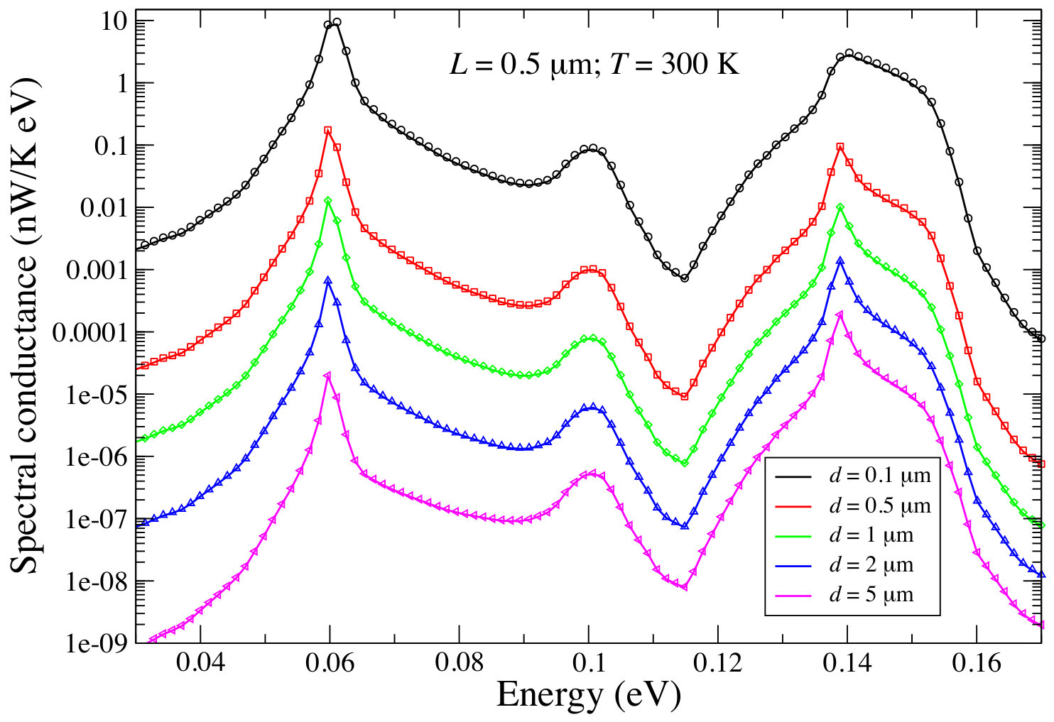 Figure 1
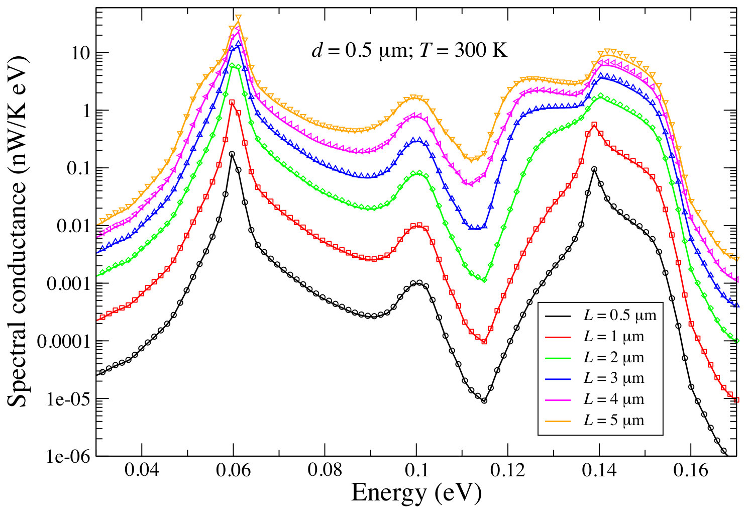 Figure 2
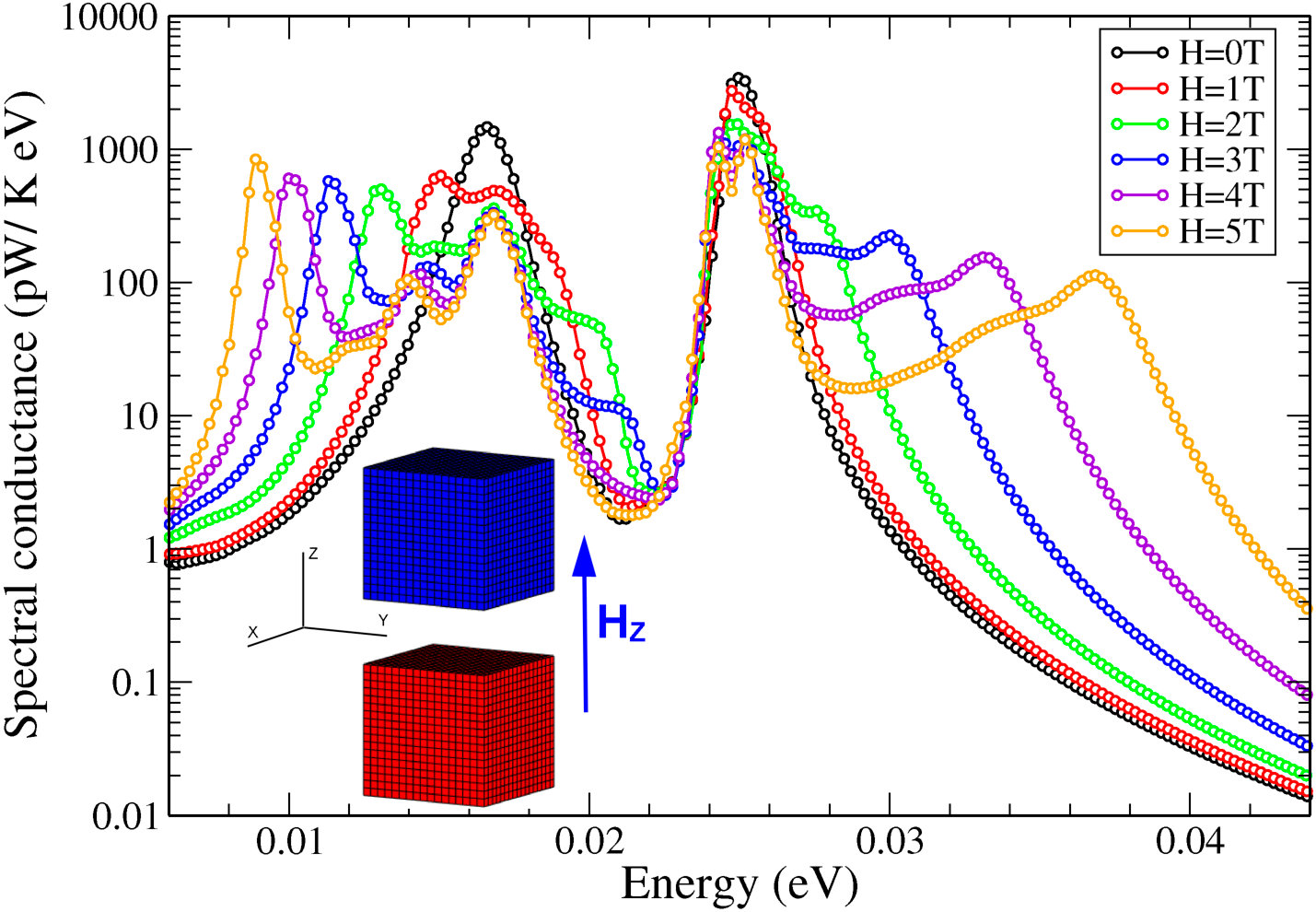 Figure 3
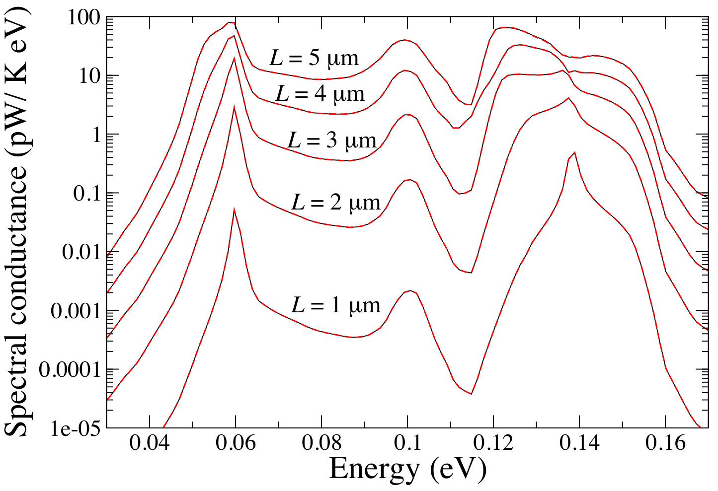 Figure 4
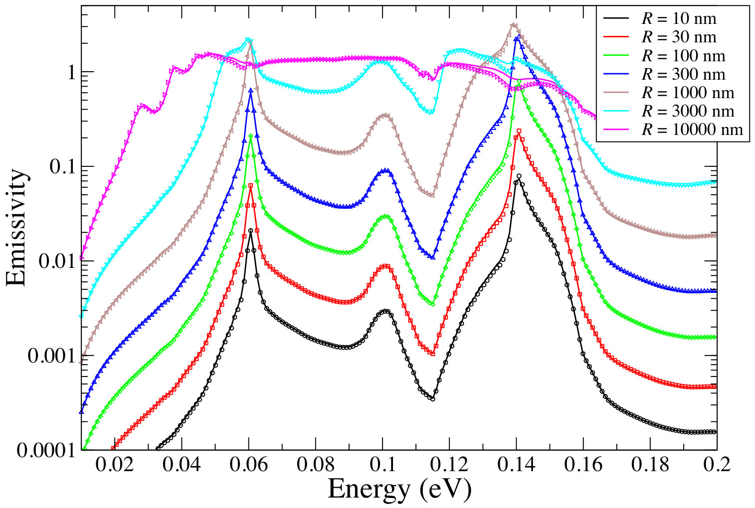 Figure 5
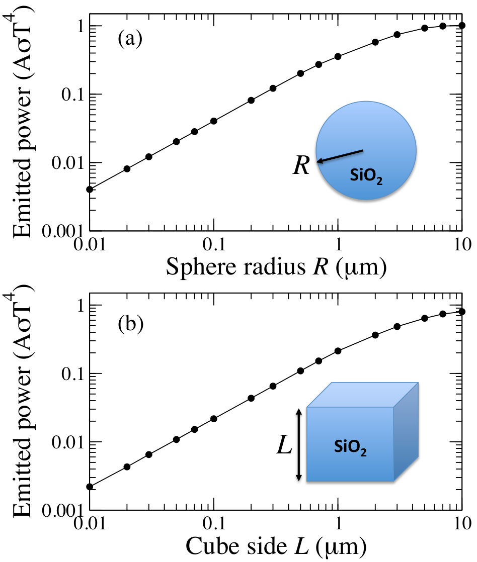 Figure 6
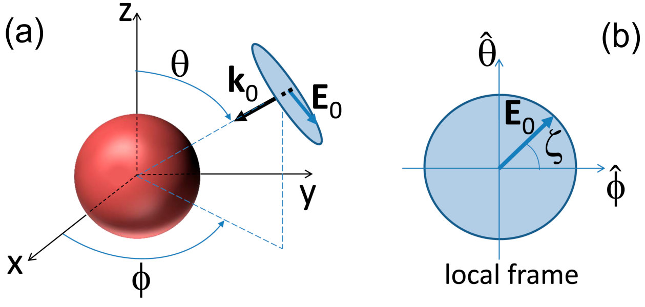 Figure 7
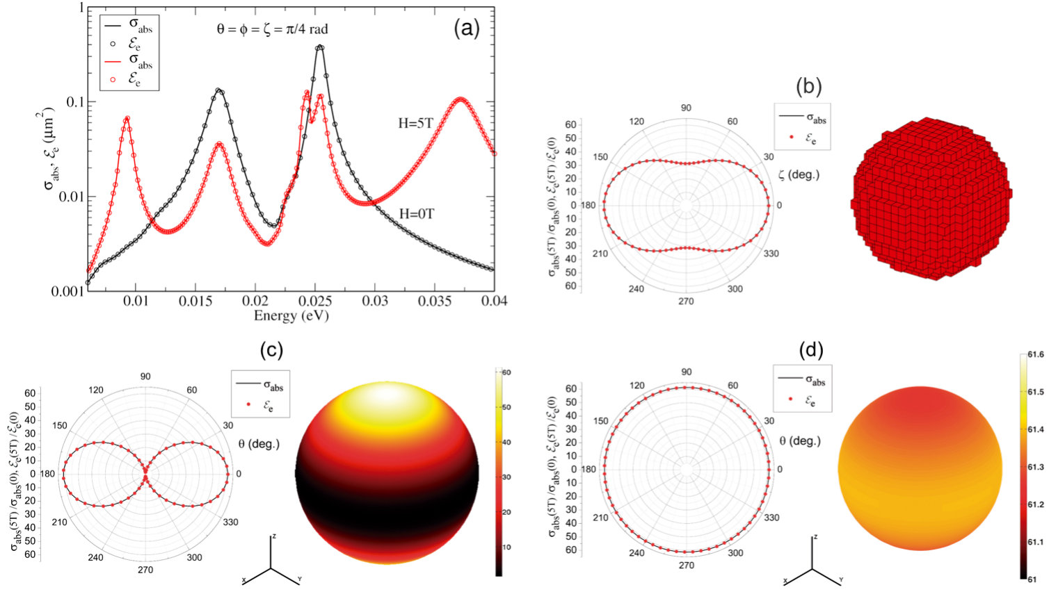 Figure 8
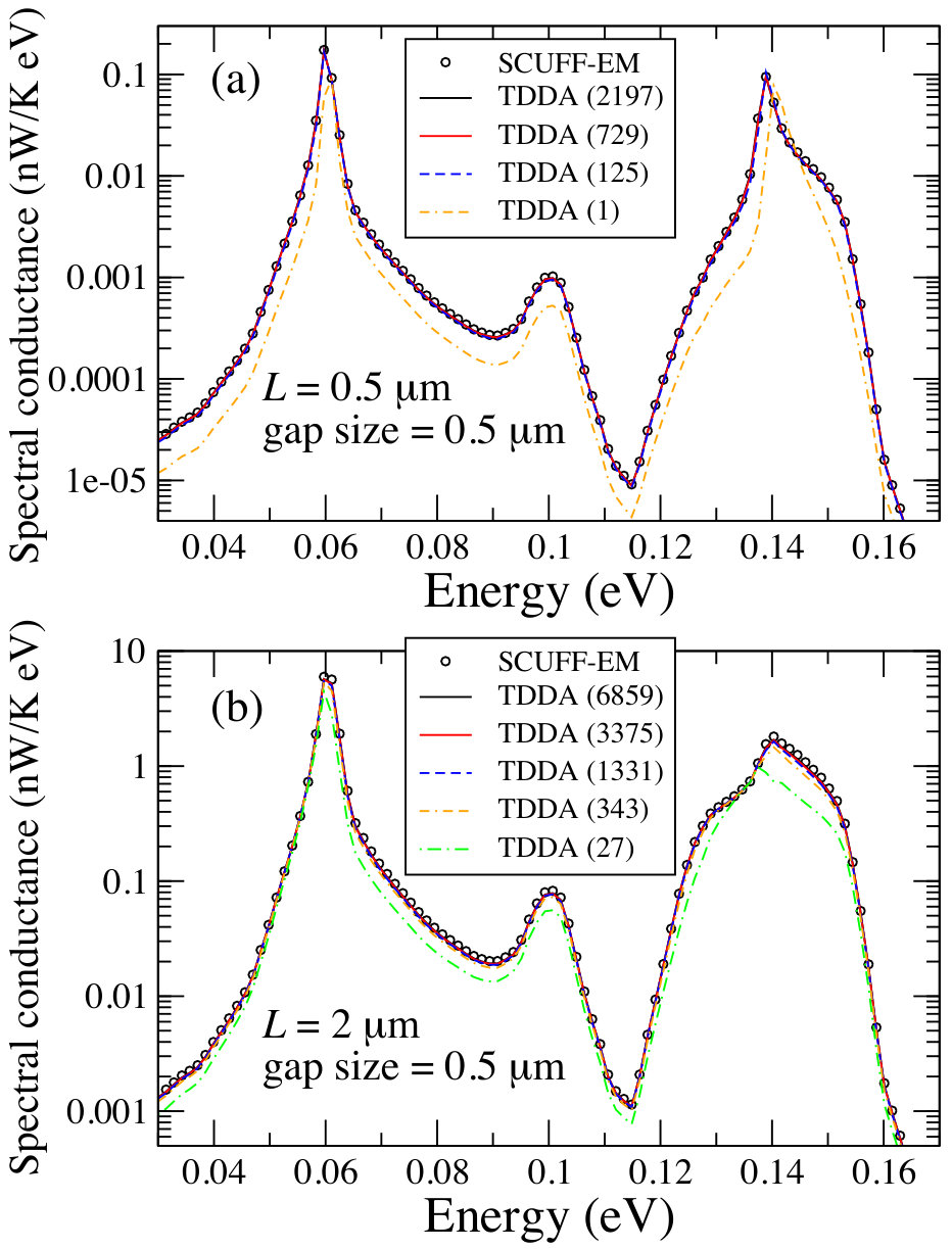 Figure 9
Peer Reviews
No public reviews on file for this paper yet. If you reviewed it on a platform where reviews are public (OpenReview, ICLR, NeurIPS, ICML), you can paste yours below so the community can read it here.
Videos
No videos yet. Explain this paper in a talk, walkthrough, or lecture? Add one.
Thermal discrete dipole approximation for the description of thermal emission and radiative
heat transfer of magneto-optical systems
R. M. Abraham Ekeroth1,2
A. García-Martín1
J. C. Cuevas3,4
1IMM-Instituto de Microelectrónica de Madrid (CNM-CSIC), Isaac Newton 8, PTM, Tres Cantos, E-28760 Madrid, Spain
2Instituto de Física Arroyo Seco, Universidad Nacional del Centro de la Provincia de Buenos Aires, Pinto 399, 7000 Tandil, Argentina
3Departamento de Física Teórica de la Materia Condensada and Condensed Matter Physics Center (IFIMAC), Universidad Autónoma de Madrid, E-28049 Madrid, Spain
4Department of Physics, University of Konstanz, D-78457 Konstanz, Germany
Abstract
We present here a generalization of the thermal discrete dipole approximation (TDDA) that allows us to describe the near-field radiative heat transfer between finite objects of arbitrary shape that exhibit magneto-optical (MO) activity. We also extend the TDDA approach to describe the thermal emission of a finite object with and without MO activity. Our method is also valid for optically anisotropic materials described by an arbitrary permittivity tensor and we provide simple closed formulas for the basic thermal quantities that considerably simplify the implementation of TDDA method. Moreover, we show that employing our TDDA approach one can rigorously demonstrate Kirchhoff’s radiation law relating the emissivity and absorptivity of an arbitrary MO object. Our work paves the way for the theoretical study of the active control of emission and radiative heat transfer between MO systems of arbitrary size and shape.
I Introduction
There is presently a great interest in the study of the radiative heat transfer between closely placed objects Song2015b . The reason for that is the experimental verification of the prediction that the radiative heat transfer between two bodies can be greatly enhanced when they are brought sufficiently close to each other Polder1971 ; Rytov1953 . This enhancement can lead to overcome the far-field limit set by the Stefan-Boltzmann law for black bodies and it takes place when the gap between the two objects is smaller than the thermal wavelength (9.6 m at room temperature). Such an enhanced thermal radiation exchange originates from the contribution of evanescent waves that dominate the near-field regime and by now it has been observed in numerous experiments Kittel2005 ; Rousseau2009 ; Shen2009 ; Ottens2011 ; Kralik2012 ; Zwol2012a ; Zwol2012b ; Guha2012 ; Worbes2013 ; St-Gelais2014 ; Song2015a ; Kim2015 ; St-Gelais2016 ; Song2016 ; Bernardi2016 ; Cui2017 . These experiments have in turn triggered off the hope that near-field radiative heat transfer (NFRHT) could lead to new applications in the context of thermal technologies such as thermophotovoltaics Laroche2006 ; Lenert2014 ; Bierman2016 , heat-assisted magnetic recording Challener2009 ; Stipe2010 , scanning thermal microscopy Wilde2006 ; Kittel2008 ; Jones2013 , nanolithography Pendry1999 or thermal management Otey2010 ; Ben-Abdallah2014 , just to mention a few.
The theoretical description of NFRHT is usually done in the framework of fluctuational electrodynamics (FE) introduced by Rytov in the 1950s Rytov1953 ; Rytov1989 . In this framework, it is assumed that the thermal radiation is generated by random, thermally activated electric currents in the interior of a material. These currents vanish on average, but their correlations are given by the fluctuation-dissipation theorem Landau1980 ; Keldysh1994 ; Joulain2005 . Thus, the technical problem involved in the description of the radiative heat transfer between two finite objects is to find the solution of the stochastic Maxwell equations with random electric currents as radiation sources. This problem can be quite challenging and an analytical solution can only be obtained in a few cases with simple geometries like, for instance, two parallel plates Polder1971 , two spheres Narayanaswamy2008 or a sphere in front of a plate Otey2011 . In general, in order to solve this problem for complex geometries, which is usually necessary for a comparison with the experiments, one has to resort to numerical methods. In this respect, a lot of progress has been done in recent years and standard numerical methods in electromagnetism have already been combined with FE to describe NFRHT between objects of arbitrary size and shape (for a review see Ref. Otey2014 ). Those methods include, among others, the scattering matrix approach Kruger2011 ; Kruger2012 , finite-difference time- and frequency-domain methods Rodriguez2011 ; Liu2013 ; Datas2013 ; Wen2010 , the boundary element method Rodriguez2012 ; Rodriguez2013 , and volumen-integral-equation methods Polimeridis2015 . Recently Francoeur and coworkers adapted the discrete dipole approximation (DDA) to describe the NFRHT between two optically isotropic objects of arbitrary shape Edalatpour2014 ; Edalatpour2015 ; Edalatpour2016 . This new approach has been termed as thermal discrete dipole approximation (TDDA). It describes the NFRHT between two bodies in the framework of FE by discretizing the objects in terms of point dipoles in the spirit of the DDA method that is widely used for describing the scattering and absorption of light by small particles Purcell1973 ; Draine1988 ; Draine1994 ; Yurkin2007 . The goal of this work is to generalize the TDDA method to describe the radiative heat transfer and the thermal emission in magneto-optical (MO) systems.
MO objects are of great interest in the context of NFRHT. Thus for instance, in a recent work by some of us we showed that the NFRHT between two parallel plates made of doped semiconductors can be largely tuned by applying a static external magnetic field Moncada-Villa2015 . Doped semiconductors under a magnetic field present a sizable MO activity, that can be controlled by changing the magnitude and the direction of the field. More recently, it has been predicted that the NFRHT between several MO particles, also made of doped semiconductors, can lead to the appearance of striking phenomena such a near-field thermal Hall effect Ben-Abdallah2016 or the existence of a persistent directional heat current Zhu2016 .
Motivated by these recent developments in the context of NFRHT of MO systems, we present here a generalization of the TDDA method to describe the radiative heat transfer between MO objects of arbitrary shape, something that is still missing in the literature. To be precise, we present a TDDA method that is valid for optically anisotropic systems that can be described by an arbitrary electric permittivity tensor (with ). We also extend the TDDA approach to describe the thermal emission of a finite object (both MO and non-MO). Moreover, we use our generalized approach to provide a rigorous demonstration of the Kirchhoff law relating the emissivity and absorptivity of a finite MO object. Finally, we also provide the correct expression for the radiative heat transfer between MO dipoles, which is the basis to study many-body effects in systems of non-reciprocal particles. Our work focuses on the analysis of homogeneous MO objects with constant temperatures, but it can be straightforwardly generalized to more complicated situations including the description of nonhomogeneous materials or situations with complicated temperature profiles. Our work provides a practical method to investigate many interesting effects in the context of the thermal emission and NFRHT between MO systems.
The rest of the paper is organized as follows. In section II we review the DDA method for MO systems that we use as a starting point for our generalized TDDA approach. Section III is devoted to the description of the radiative heat transfer between MO dipoles. In section IV we describe in detail our generalized TDDA approach for the description of the radiative heat transfer between two MO bodies. In section V we show how the TDDA can be used to describe the total thermal emission of an arbitrary finite object. In section VI we address the issue of the Kirchhoff law of thermal radiation of MO objects. In particular, we derive here the definition of the directional, polarization-dependent emissivity that has to be compared with the corresponding absorption cross section to prove Kirchhoff’s law. In section VII we present the numerical results obtained for the thermal radiation and radiative heat transfer between different objects of arbitrary size and shape. The goal of this section is to illustrate both the validity and the capabilities of the formalisms developed in the previous sections. We conclude the paper in section VIII with some additional remarks about our TDDA approach and the main conclusions of our work. On the other hand, we have included two appendixes where we briefly discuss the convergence of the method (Appendix A) and provide an alternative derivation of the main result of section IV (Appendix B).
II DDA for magneto-optical systems: A reminder
Our formulation of the TDDA is based on a DDA extension to describe the electromagnetic response of MO systems that has been recently put forward by one of us deSousa2016 . To make this paper more self-contained, we present here a brief description of this method, which in turn will allow us to illustrate the peculiarities of the DDA approach for MO objects.
Let us recall that a MO system is characterized by a non-symmetric permittivity tensor whose components depend on an external magnetic field or on the magnetization state. With this idea in mind, we consider an optically anisotropic finite object characterized by a spatially-dependent dielectric permittivity tensor that is embedded in a homogeneous medium, which hereafter is assumed to be vacuum. In the absence of currents inside the object, the electric field is given by the solution of the volume-integral equation Novotny2012
[TABLE]
Here, is source electric field or the field in the absence of the object, is the magnitude of the vacuum wave vector, is the volume of the object, and is the vacuum dyadic Green tensor given by Novotny2012
[TABLE]
where , , and denotes the exterior product.
In the DDA approach, the previous integral equation is solved by discretizing the volume as , where is the volumen of an homogeneous region where the electric field is assumed to be constant. Thus, Eq. (1) now reads
[TABLE]
Defining the dipole moments as
[TABLE]
we can rewrite Eq. (3) as
[TABLE]
where
[TABLE]
It can be shown that deSousa2016
[TABLE]
and
[TABLE]
Here, is the so-called electrostatic depolarization dyadic that depends on the shape of the volume element Lakhtakia1992 ; Yaghjian1980 . For the case of a parallelepiped of volume , adopts the form Yaghjian1980
[TABLE]
Thus, we can now rewrite Eq. (5) for the internal field, , as follows
[TABLE]
where , and .
The left hand side of Eq. (II) can be defined as the exciting field , i.e., the field that excites the -volumen element. Now, defining the polarizability tensor of the -volumen element, , as
[TABLE]
where
[TABLE]
is the quasistatic polarizability tensor, Eq. (II) can be rewritten as a set of coupled dipole equations for the exciting fields at each element
[TABLE]
It is worth stressing that this DDA formulation includes automatically the so-called radiative corrections Sipe1974 ; Belov2003 ; Albaladejo2010 , which are related to the imaginary part of the Green tensor, and it is thus fully consistent with the optical theorem. On the other hand, from the solution of Eq. (13), which constitutes a set of 3 coupled linear equations for the exciting fields, one can get the dipole moments and the total internal fields as follows
[TABLE]
Let us conclude this section with a few useful remarks. First, for cubic volumen elements, the depolarization tensor is diagonal: . For volumen elements of spherical or cubic, optically isotropic materials, the polarizability tensor is diagonal: with
[TABLE]
Finally, from the knowledge of the dipole moments and the internal fields, one can easily compute the different cross sections (scattering, absorption, and extinction). In particular, the absorption cross section, which will play an important role later on, can be obtained as follows. Assuming a plane-wave illumination, , the absorption cross section is given by deSousa2016
[TABLE]
III Radiative heat transfer between magneto-optical dipoles
Before presenting our generalized formulation of the TDDA for arbitrary bodies, it is instructive to first discuss the radiative heat transfer between MO dipoles. This discussion will allow us to highlight the peculiarities of MO systems.
The problem that we address in this section is the radiative heat transfer (both in the near and in the far field) between two MO particles that are small compared to their thermal wavelengths such that they can treated as point electrical dipoles. Let us assume that these two dipoles (or dipolar particles) are located in positions and , they have arbitrary polarizability tensors and , and they are at temperatures and . To compute the net power exchanged between the two dipoles, we first compute the power dissipated in dipole 2 due to the emission from dipole 1, , assuming that dipole 2 does not emit note1 . This power is given by
[TABLE]
where is the local electric current density in the volume and is the local electric field at position . Moreover, denotes the statistical average that takes into account the stochastic nature of the dipoles. Let us recall that the thermal emission originates from the fluctuating part of the dipole moments.
Now, we can express and in terms of their Fourier transforms
[TABLE]
Using the fact that these two functions are real, one can easily show that
[TABLE]
Since the fluctuation-dissipation theorem (FTD) will introduce a -function of the type , we focus on the calculation of and in most cases we shall drop the argument to alleviate the notation.
In order to determine the dipole moment and field, we need to solve the DDA equations, see Eq. (13). The exciting field at the position of dipole 2 is given by
[TABLE]
To close this equation, we need the corresponding equation for , which reads
[TABLE]
Notice that there is no source term in this case. Introducing Eq. (21) in Eq. (20), we arrive at
[TABLE]
where
[TABLE]
The source field , due to the emission of the fluctuating part of dipole 1, , is given by . Thus,
[TABLE]
where we have defined .
Now, using Eqs. (14) and (15), we can express the dipole moment and the internal field in terms of as
[TABLE]
To compute it is convenient to use a matrix notation where column vectors like are understood as () matrices and row vectors like are () matrices. With this notation, we get rid of the dot product (or scalar product) in favor of matrix multiplications as follows
[TABLE]
Now, using Eqs. (11) and (12) it is easy to show that
[TABLE]
Introducing this relation into Eq. (III) and after several simple algebraic manipulations, we arrive at
[TABLE]
where
[TABLE]
Notice that .
Now, making use of Eq. (24), we obtain
[TABLE]
The statistical average appearing in the previous equation can be determined with the help of the fluctuation-dissipation theorem (FDT), which in its most general form reads Landau1980 ; Keldysh1994 ; Joulain2005
[TABLE]
where is the Bose function. Several remarks are pertinent at this stage. First, notice that the FDT of Eq. (31) involves , which contains two terms, see Eq. (29). The first one is the standard contribution, while the second one is related to the radiative correction and its contribution avoids the violation of the optical theorem Manjavacas2012 . The origin of this term has been nicely explained by Messina et al. Messina2013 and the result above is a generalization of their arguments to the MO case. On the other hand, notice that in the first term in the expression of the combination appears, which for MO systems differs from . This latter combination was used in the work of Ref. [Nikbakht2014, ] for the description of radiative heat transfer between anisotropic particles and therefore, that formulation is not valid for MO systems, as it was assumed in the work on the photon thermal Hall effect of Ref. [Ben-Abdallah2016, ].
Now, we can combine Eqs. (31), (30), and (III) to write the power dissipated in dipole 2 due to the emission from dipole 1 as follows
[TABLE]
Following the same line of reasoning, one can show that the power absorbed by the particle 1 due to the emission of particle 2 is given by
[TABLE]
where can be obtained from by interchanging the indexes 1 and 2.
It is straightforward to show that
[TABLE]
Thus, the net power exchange, , between the two particles is given by the Landauer-like formula
[TABLE]
where and is the frequency-dependent transmission function given by
[TABLE]
We emphasize that this result differs from that reported in Refs. [Nikbakht2014, ; Ben-Abdallah2016, ] and it only coincides with those results for non-MO particles. It is also important to remark that in the case of isotropic particles, it reduces to the result reported in the literature in which radiative corrections have been taken into account Manjavacas2012 ; Messina2013 .
IV Generalized TDDA: Radiative heat transfer between two arbitrary
magneto-optical bodies
In this section we present our generalized TDDA for the description of the radiative heat transfer between MO objects of arbitrary shape and for arbitrary separations. In particular, we focus here on the case of two finite objects assumed to be at fixed temperatures and and do not consider the interaction with any thermal bath.
In the spirit of the DDA, we assume that these two bodies are described by a collection of (body 1) and (body 2) electrical point dipoles. Each dipole is characterized by a volumen and a polarizability tensor , where indicates to which body the dipole belongs and if and if . The information about the individual dipole moments and the internal electrical field can be grouped into column supervectors (denoted with a bar) as follows
[TABLE]
[TABLE]
The same notation will be used for the exciting and source electric fields.
The calculation of the net radiative power exchanged by arbitrary objects is a straightforward generalization of the calculation for two dipoles presented in the previous section and we shall follow the same strategy. Thus, we first compute the power absorbed by object 2 due to the thermal emission of object 1, , which is given by
[TABLE]
Following the previous section, the goal is now to compute the exciting field . For this purpose, we use Eq. (13), which can be rewritten in a more compact form using the notation above
[TABLE]
Here, with
[TABLE]
where is the vacuum dyadic Green tensor connecting dipole in body with dipole in body and with .
Solving now for , we have
[TABLE]
where
[TABLE]
The source field, , due to the emission of the fluctuating dipoles in body 1, , is given by
[TABLE]
Thus,
[TABLE]
From Eq. (46) it is easy to show that
[TABLE]
Therefore,
[TABLE]
where
[TABLE]
Now, we use Eqs. (14) and (15) to express the dipole moment and the internal field in terms of as
[TABLE]
where .
Following the same steps as in the previous section, it is straightforward to show that
[TABLE]
where with . Let us recall that is given by Eq. (29). Again, the statistical average appearing in the previous equation can be computed with the FDT, which now reads
[TABLE]
Now, we can combine the last two equations to write the power dissipated in body 2 due to the emission from body 1 as follows
[TABLE]
Analogously, one can show that the power absorbed by body 1 due to the emission of body 2 is given by
[TABLE]
where can be obtained from by interchanging the indexes 1 and 2.
On the other hand, it can be shown that
[TABLE]
Thus, the net power exchange, , between the two bodies is given by the Landauer-like formula
[TABLE]
where let us recall that and is the transmission function given by
[TABLE]
Eqs. (59) and (60) are our central result for the description of the radiative heat transfer between anisotropic objects of arbitrary shape, which is valid in particular for MO systems. Obviously, the result summarized in these equations reduces to that of Eqs. (35) and (36) for the case of two dipoles.
The result of Eqs. (59) and (60) is valid for arbitrary separations between the two bodies, i.e., it includes both the near-field and the far-field contributions. In the far-field, the formula can be simplified by neglecting the multiple scattering between the two bodies. This can be done by approximating the matrix by
[TABLE]
Let us conclude this section by saying that our derivation of the result for the radiative heat transfer between two finite objects is based on an intuitive division of the problem into two subproblems in which one object is assumed to be the emitter and the other one the receiver, and in each subproblem the receiver is assumed to not radiate. This is indeed the strategy followed by Polder and van Hove in their seminal paper in which they computed the radiative heat transfer between two parallel plates Polder1971 . Anyway, one might wonder if this ad hoc division is fully justified in the problem addressed in this section. To demonstrate that this is indeed the case, we present in Appendix B an alternative derivation of the central result of this section starting from a different point of view in which both objects radiate “simultaneously” and the net exchanged power is directly calculated. This alternative derivation detailed in Appendix B confirms the validity of the central result of this section summarized in Eqs. (59) and (60).
V Thermal emission of finite object
The thermal emission of a finite object is another important issue that can be described with the help TDDA, but it has not been done so far. The goal of this section, and the next one, is to fill this gap. We divide our discussion of the formulation of thermal radiation within TDDA into two parts. The first one is addressed in this section, where we present a convenient way to compute the total radiation power emitted by a finite object. The analysis of the angular and polarization dependence of the thermal emission will be carried out in the next section, where, in particular, we generalize Kirchhoff’s law of thermal radiation to the case of MO objects of arbitrary size and shape.
The problem we want to address in this section is the calculation of the total radiation power emitted by a finite body at temperature . In this case, we model this body as a collection of point dipoles that interact with the electric field of a thermal bath at temperature . The total power emitted by the body, , must be equal to the total power absorbed from the bath when they are at the same temperature. Thus, we can follow the previous section and write the emitted power as
[TABLE]
where we are using the same type of notation as in the previous section, i.e.,
[TABLE]
In this problem, the source field is the field of the bath, i.e., , where we have used the notation of previous equation. Thus, the exciting field is simply given by
[TABLE]
where . Here, , where is the vacuum dyadic Green tensor connecting dipole with dipole inside the body and .
As in the previous section, it is straightforward to show that
[TABLE]
where . Now, to compute the statistical average appearing in the previous equation, we make use of the FDT theorem for the field correlations of the bath, which reads Messina2013
[TABLE]
Now, we can combine the last two equations to write the emitted power as follows note2
[TABLE]
where
[TABLE]
is Planck distribution function. In the previous equation one can identify
[TABLE]
as a quantity that, when divided by the geometrical cross section of the body, plays the role of an effective angular-averaged frequency-dependent emissivity. In the case of a single dipole, , which for a spherical, optically isotropic dipole () reduces to , where is given by Eq. (16). As we show below, the quantity is simply the absorption cross section of this isotropic dipole.
VI Kirchhoff law of thermal radiation of magneto-optical objects
Another fundamental question that we want to address in this work is the validity of Kirchhoff’s law for finite MO objects. This thermal radiation law states that the emissivity is equal to the absorptivity. This law is a textbook result for the case of extended systems, but its proof for finite objects has also been reported for both isothermal bodies Rytov1989 and non-isothermal ones Greffet2016 . However, these proofs are restricted to reciprocal objects, i.e., objects with symmetric permittivity tensors, and our goal is to extend the analysis of the validity of this law to the case of MO (non-reciprocal) objects.
In its most general form, Kirchhoff’s law involves the thermal emission in a given direction and for a given polarization. Thus, our first task is to find a proper expression for the polarization-dependent directional emissivity. For this purpose, it is convenient to write the total emitted power in a way different than above, i.e., in terms of Poynting’s vector as
[TABLE]
which describes the integrated flux across a differential section perpendicular to a radial unit vector , performed over a sphere of radius enclosing the emitting object. Since this quantity does not depend on the actual choice of , for convenience, we will evaluate Poynting’s vector in the far field.
Now, we need to compute the statistical average of Poynting’s vector resulting from the thermal emission of an arbitrary body, i.e., , where is the point of observation (outside the object) and and are the electric and magnetic field, respectively. As usual, we can express this average in terms of the Fourier transforms of the fields as
[TABLE]
Anticipating that the FDT theorem will introduce a -function of the type , we shall focus on the calculation of and we shall not write explicitly the argument .
It is worth noting that , in virtue of the superposition principle, can always be described in terms of two linearly polarized fields that are perpendicular to each other, both lying on a plane perpendicular to , as .
In the spirit of the TDDA, we assume that our body is described by a collection of point dipoles located at positions . Using the notation of previous sections, the electric field generated by these dipoles is given by
[TABLE]
where we have defined the following row supervector of Green tensors
[TABLE]
As usual, is the source field that originates from the fluctuating dipoles inside that body and is given by
[TABLE]
The total dipole moments can be obtained from the exciting field inside the body as , while fulfills the DDA equation
[TABLE]
where . Solving for , we obtain that
[TABLE]
from which it is straightforward to show that the total field is given by
[TABLE]
where
[TABLE]
In the far-field region, the magnetic field is simply related to the electric field via
[TABLE]
where .
Now, to select the contribution of a given polarization, we write the electric field as , where is a unit vector defining the polarization state and lies in a plane perpendicular to the radial direction . In our matrix notation, the field amplitude reads and we have
[TABLE]
which with the help of Eq. (77) can be written as
[TABLE]
Now, we can make use of the FDT to write
[TABLE]
which leads to the following expression for the radial component of Poynting’s vector for a polarization given by the unit vector
[TABLE]
Let us stress that in the previous expression one must use the far-field expression of the Green tensors, i.e., where , , and .
Taking into account the standard definition of the total emitted power
[TABLE]
we can write
[TABLE]
Equation (VI) can be written as
[TABLE]
where is the polarization-dependent directional emissivity given by
[TABLE]
Let us stress that, as defined here, this emissivity has dimensions of area like the absorption cross section. On the other hand, it is worth noting that Eq. (86) permits establishing the following relationship between the total emissivity and the polarization-dependent directional emissivity
[TABLE]
where it is easy to verify that in the case of isotropic it reduces to .
The quantity has to be compared with the absorption cross section for the same polarization and incident angle to verify Kirchhoff’s law. The expression for the absorption cross section is given by Eq. (17), which can be written as
[TABLE]
where
[TABLE]
is a linearly polarized plane wave impinging as .
A general demonstration of Kirchhoff’s law from Eqs. (87) and (89) is cumbersome. In what follows we will provide evidence of this fulfillment in the case of single dipoles whereas a numerical verification for finite objects will be provided in section VII.
In the case of a single dipole we have that in Eq. (87) and in Eq. (89). Then, using , the absorption cross section can be written as . On the other hand, if we assume that the dipole is located at the origin of the spherical coordinate system, the Green tensor in far-field approximation is given by and Eq. (87) becomes
[TABLE]
Finally, for an isotropic system this leads to the well-known Kirchhoff’s result.
VII Numerical results
In this section we present a series of results related to the different aspects of radiative heat transfer and thermal emission discussed in previous sections. Our goal is to illustrate the capabilities of the TDDA method put forward in this work, as well as to demonstrate its validity by comparing with established results in the literature. For these purposes, we shall consider below two materials. First, as an example of a non-MO material we choose SiO2, which is polar dielectric that has been amply studied in the context of NFRHT. We use the dielectric function of SiO2 reported in Palik’s book Palik1985 . As an example of a MO material we shall consider -doped InSb, a polar semiconductor, that when subjected to an external magnetic field becomes MO. For the sake of concreteness, we shall assume that magnetic field is applied in the -direction, . In this case, the permittivity tensor of InSb adopts the following form Palik1976
[TABLE]
where
[TABLE]
Here, is the high-frequency dielectric constant, is the longitudinal optical phonon frequency, is the transverse optical phonon frequency, defines the plasma frequency of free carriers of density and effective mass , is the phonon damping constant, and is the free-carrier damping constant. Finally, the magnetic field enters in these expressions via the cyclotron frequency . Let us point out that in this case the magneto-optics is induced by the magnetic field, which modifies the diagonal elements of the permittivity tensor and introduces off-diagonal terms. There are two contributions to the diagonal components, namely, optical phonons and free carriers. These latter ones are responsible for the magneto-optics at finite magnetic field. Notice that we have neglected the contribution from intra-band transitions because we are interested in thermal properties at room temperature, where this contribution does not play any role. In all calculations below, we consider the particular case taken from Ref. [Palik1976, ], where , rad/s, rad/s, rad/s, rad/s, cm*-3*, , and rad/s. As a reference, let us say that with these parameters rad/s for a field of 1 T.
The explicit form for the dielectric tensor given by Eq. (92) gives rise to a , see Eq. (29), having the form
[TABLE]
For simplicity, the results presented below are for homogeneous bodies, i.e., with a spatially constant permittivity tensor, and for constant temperatures inside the bodies. Moreover, all the results for finite systems were obtained by discretizing the objects in terms of cubes of equal size. The corresponding polarizability tensors of the cubes were computed with Eqs. (11) and (12) with , which in the case of isotropic materials reduce to Eq. (16). Unless stated otherwise, the calculations of the radiative thermal conductance, power emission, etc., were carried out at K.
VII.1 Radiative heat transfer
The issue that we want to address now is the description of the radiative heat transfer between two finite objects using the formalism detailed in section IV. To test the validity of this formalism, we first consider the case of optically isotropic objects, a case that can be described with existent methods. Indeed, in this case our formalism basically reduces to the TDDA put forward in Ref. [Edalatpour2015, ], which was thoroughly tested against the solution for two spheres Narayanaswamy2008 . In our case, and in order to avoid known problems related to the so-called shape error, an error due to the description of objects that cannot be exactly represented by cubical lattices Draine1988 ; Yurkin2006 , we consider here the heat transfer between two identical cubes of side . In Fig. 1 we show as solid lines the TDDA results for the spectral radiative thermal conductance (conductance per unit of energy) as a function of the photon energy for two SiO2 cubes of side m and various separations ranging from 100 nm to 5 m. To check the validity of our TDDA approach, we compare our results with those obtained with the code SCUFF-EM Reid2015 ; SCUFF-EM , which are shown in Fig. 1 as open symbols. The SCUFF-EM solver implements the fluctuating-surface-current (FSC) formulation of the heat transfer problem put forward in Refs. [Rodriguez2012, ; Rodriguez2013, ] in combination with the boundary element method (BEM). The FSC-BEM combination used in SCUFF-EM enables the description of the radiative heat transfer between homogeneous, optically isotropic bodies of arbitrary shape and provide numerically exact results within the framework of fluctuational electrodynamics in the local approximation, i.e., assuming that the dielectric function only depends on frequency.
As it can be seen in Fig. 1, our TDDA method is able to reproduce the exact results obtained with SCUFF-EM. Let us say that the TDDA results shown here were obtained modeling each cube with 6859 cubic dipoles (we briefly discuss the convergence of these results with the number of dipoles used in the simulations in Appendix A). It is worth stressing that it becomes progressively more demanding to converge the TDDA results upon reducing the gap between the cubes. Thus for instance, in this example the difference between the TDDA and the SCUFF-EM results for the total conductance (integrated over energy) is of 2.5% for a gap of m, while it monotonically increases up to 6.2% for nm. The physical reason for this behavior is the fact that the NFRHT in this case is dominated by surface phonon polaritons Mulet2002 that have a penetration depth comparable to the gap size Song2015a . This implies that the electric field inside the cubes varies on a length scale smaller than the gap and therefore, one needs an increasing number of dipoles to properly describe the radiative heat transfer as the gap diminishes. The important thing is that the error in the TDDA calculations can be systematically reduced by refining the dipole grid, which can be done by increasing the number of dipoles or using adaptive meshes. Let us stress that in this work we are not interested in presenting a detailed analysis of the convergence of our TDDA approach (since it would be strictly equivalent to that in Ref. Edalatpour2015 ), but rather in establishing its fundamental validity.
We present another example of the comparison between our TDDA results and those obtained with SCUFF-EM for the spectral conductance of two SiO2 cubes of varying size and gap m in Fig. 2. Again, we find a very good agreement between both types of results, which becomes progressively worse (for a fixed number of dipoles) as the side of the cube increases, as expected. More importantly, we always find that this agreement can be systematically improved by increasing the number of dipoles in our cubic lattices (for more details on the convergence of these results, see Appendix A). So in short, we conclude that our TDDA method produces the correct results for the radiative heat transfer provided that a sufficiently large number of dipoles is employed in the discretization of the objects.
We now proceed to illustrate our approach in the case of MO objects, which is out of the scope of existent methods. For this purpose, we consider the radiative heat transfer between two identical InSb cubic particles of side m separated nm using 4913 cubic dipoles for each particle. The results for the spectral conductance for different values of the external magnetic field, , are shown in Fig. 3. In this case, the magnetic field is oriented as shown in the inset of this figure. As one can see, the spectral conductance in the absence of field () is dominated by the contribution of two peaks that, as explained in Ref. Moncada-Villa2015 , are due to the contribution of surface plasmon polaritons (low-energy peak) and surface phonon polaritons (high-energy peak). Notice that the magnetic field induces a splitting of the low-energy peak, while it introduces a new peak at high energies that appears at the cyclotron frequency and therefore, its position is blue-shifted linearly with the external field. This behavior is very similar to what it was found in Ref. Moncada-Villa2015 for the case of two semi-infinite InSb plates. These results will be discussed in more detail in a forthcoming publication and we show them here just to illustrate the capabilities of our TDDA method.
To conclude this subsection, we want to illustrate the validity of the far-field approximation of Eq. (61). For this purpose, we show in Fig. 4 a comparison between the exact results and the far-field approximation for the room temperature spectral conductance for two identical cubes of SiO2 of various sizes separated a distance of 20 m, which is larger than the thermal wavelength. The results were computed with 2197 dipoles in each cube, which was sufficient to converge the results with an accuracy of better than 1%. As it is clear from Fig. 4, the approximation of Eq. (61) accurately reproduces the exact results.
VII.2 Total thermal emission
In this subsection we want to discuss the total thermal emission of a finite object. To test the validity of the formalism described in section V we first consider the total thermal emission of a sphere of a non-MO material. A well-known result, first derived by Kattawar and Eisner Kattawar1970 , is that the emissivity of a non-MO sphere of arbitrary radius obtained within fluctuational electrodynamics is equal to the corresponding absorption efficiency, i.e., to the absorption cross section normalized by the geometrical cross section. Let us recall that we demonstrated this result in section V for the case of a single spherical dipole. Since the absorption efficiency can be computed exactly with the help of Mie theory Bohren1998 , the result of Kattawar and Eisner provides a very stringent test for our theory of thermal emission. We have computed both the emissivity and absorption efficiency using Eqs. (69) and (89), respectively, for spheres of different sizes and materials and in all cases we have found that they are indeed identical. In Fig. 5 we show the TDDA results for the total emissivity of a SiO2 sphere for different radii (solid lines) as a function of the energy. Let us clarify that we are showing the quantity defined in Eq. (69) and normalized by the geometrical cross section to make it dimensionless. We also show the corresponding results for the absorption efficiency calculated with the exact Mie theory Bohren1998 . As one can see, there is a very good agreement between our TDDA results and the exact results, which demonstrates the validity of our formalism. Again, it is worth remarking that as one increases the size of the sphere, a larger number of dipoles is required to satisfactorily converge the results. To obtain the results of Fig. 5 we used about 12000 dipoles, which is enough to reproduce the exact results for spheres of radius up to approximately 10 m. In any case, it is important to emphasize there is no fundamental limitation to obtain the exact result within our TDDA approach, although the practical problem to converge the results may become in some cases very difficult to overcome.
For completeness, we show in Fig. 6 the total power emitted at room temperature by a sphere and a cube of SiO2 of varying size. The results are normalized by the corresponding results for a black body (Stefan-Boltzmann law). As one can see, for small spheres and cubes the emitted power is proportional to the volumen of the finite objects. This is a well-known result Kruger2011 ; Kruger2012 , which is due to the fact that in this regime the skin depth of this material at the relevant wavelengths is larger than the characteristic size of the object. This means in practice that the whole object contributes to the thermal emission. However, as the size increases, the emitted power becomes proportional the area of the object, which reflects the fact that the size becomes larger than the skin depth and then only the surface of the object significantly contributes to the thermal emission. Notice also that in both cases (spheres and cubes), when the characteristic size becomes on the order of a few microns, the emitted power becomes comparable to that of a black body of the same size. Let us say that the thermal emission of a SiO2 sphere was studied by Krüger et al. Kruger2011 ; Kruger2012 and our results agree with those reported in those references.
VII.3 Kirchhoff’s law for MO systems
The goal of this subsection is to illustrate the validity of Kirchhoff’s law in the case of finite MO objects. But before presenting the full numerical analysis, it is instructive to consider a MO dipole (where we still consider MO activity is due to a magnetic field pointing along the -direction) since it is possible to provide an analytical solution for an arbitrary polarization vector . Using the coordinate system depicted in Fig. 7 the spectral, polarization-dependent directional emissivity for a single dipole with given by Eq. (94) can be written for any polarization angle as [see Eq. (91)]
[TABLE]
Notice that there is no dependence on the azimuthal angle due to the symmetry introduced by the fact that . Moreover, since we have to choose two orthogonal vectors, i.e., and , the sum required to obtain the total emitted power is equal to , that, as expected, does not depend on the choice of .
Since the direction of the external magnetic field imposes a preferential direction, it is convenient to choose two values of so that one polarization vector has no component along the direction of the external magnetic field, rad (let us call it ), while the other is collinear with the magnetic field, rad (let us call it ). It is straightforward to see that , i.e., independent of any incidence angle or , while presenting thus a dependence, varying from to .
To illustrate the fulfillment of Kirchhoff’s law for a body of finite size, we consider an homogeneous InSb sphere of radius m, using discretization unit cubes with an edge of nm ( 2550 discretization elements). In Fig. 8(a) we present spectra of the polarized emissivity and of the absorption cross section for a direction defined by rad and polarization angle by rad. Two values of magnetic field, T and T, are shown. For both cases and (for the same angles and polarization) are identical.
In order to analyze the same system as a function of the geometrical angles, we verify the dependence obtained for a single dipole in Eq. (95). This is clearly visible in Fig. 8(b), where we plot and for rad, rad and eV, as a function of for an applied field of T normalized to its value at T (let us point out that, since the geometry is fully isotropic, for T it happens that and thus emissivity and absorption cross section are polarization insensitive).
The next step in the verification is to compare the angular profile of the emissivity and of the absorption cross section for fixed polarizations. As it can be understood from Eq. (95), the most interesting choice is the -polarization ( rad). In Fig. 8(c), we present a colormap of and (for the same polarization) for T normalized to T, as a function of and showing that they are independent of and that the dependence on is of the form of , as evidenced by the associated polar plot. The same plot, but for -polarization is presented in Fig. 8(d) demonstrating that for this configuration and polarization, the emissivity and absorption cross section is isotropic, within a numerical error smaller than 2%.
Let us conclude this subsection by saying that we have analyzed the polarization-dependent, directional emissivity and the corresponding absorption cross section for different sizes and shapes of InSb particles under a magnetic field finding that in all cases these two quantities are identical.
VIII Additional remarks and conclusions
In this work we have focused on the description of the thermal radiation and radiative heat transfer of homogeneous objects with constant temperatures. However, all the basic formulas derived in this work are directly applicable to the case of inhomogeneous objects, with spatially dependent dielectric functions, and they can be straightforwardly generalized to consider the case of arbitrary temperature profiles in the interior of the objects. On the other hand, the TDDA method presented here can easily be generalized in a number of additional ways to treat, for instance, the radiative heat transfer between surfaces and finite objects Edalatpour2016 or between periodic systems Draine2008 .
With respect to the improvement of the efficiency and accuracy of the TDDA method presented here, there are a number of obvious improvements that one can implement without the need to modify the formulation detailed in this work. Thus for instance, one can employ adaptive dipole lattices to better describe the non-uniform field profiles inside the objects Edalatpour2015 , one can discretize the objects in terms of non-cubic dipoles with shapes better adapted to the geometries of the objects under study Smunev2015 , or one can use a DDA formulation based on the integration of the Green’s tensor (IGT) in the spirit of Ref. Chaumet2004 , rather than on the standard point-dipole interaction, as done in this work.
In summary, we have presented in this work a new formulation of the TDDA approach to describe the radiative heat between finite objects of arbitrary size and shape. This formulation allows us to describe the radiative heat transfer between MO objects and, more generally, between optically anisotropic objects with arbitrary permittivity tensors. We have shown how this TDDA approach can also be used to describe the thermal emission of a finite object. Moreover, we have provided very compact and transparent formulas for different physical quantities that can be directly employed in generalizations of the method presented here. In particular, we have corrected the existent formulas for the radiative heat transfer between non-reciprocal dipoles, which can be used to analyze different many-body effects in ensembles of MO particles. On the other hand, we have used our TDDA approach to demonstrate Kirchhoff’s law relating the emission and absorption of non-reciprocal objects. Our work opens the way for the rigorous description of different thermal radiation phenomena involving finite MO objects of arbitrary shape.
Acknowledgements.
We thank V. Fernández-Hurtado for providing the numerical results obtained SCUFF-EM shown in this paper, and J.J. Sáenz and N. de Sousa for stimulating discussions. This work was financially supported by the Comunidad de Madrid (Contract No. S2013/MIT-2740). J.C.C. also acknowledges financial support from the Spanish MINECO (Contract No. FIS2014-53488-P) and thanks the DFG and SFB 767 for sponsoring his stay at the University of Konstanz as Mercator Fellow. A.G.-M. also acknowledges funding from the Spanish MINECO (Contract No. MAT2014-58860-P).
Appendix A Convergence analysis
In this appendix we present a brief analysis of the convergence of the results shown in section VII.1. In Fig. 9 we show some convergence tests for the radiative heat transfer between two SiO2 cubes of two different sizes. In this figure, together with the converged results obtained with SCUFF-EM, we show the TDDA results obtained with different number of dipoles (per cube). As one can see, upon increasing the number of dipoles, the TDDA results first converge rapidly to approximately the correct result and then, the convergence improves slowly, but monotonically until a very satisfactory agreement with the SCUFF-EM results is achieved. Of course, as the size of the objects increases, the required number of dipoles increases accordingly and a proper convergence becomes much more demanding. The same occurs when the gap size is reduced (not shown here). In that case, the electric field inside the SiO2 particles varies more rapidly in space due to the smaller penetration depth of the surface phonon polaritons that dominate the NFRHT in this polar dielectric Song2015a . All these qualitative conclusions on the convergence trends also apply to the case of MO objects, like that considered in Fig. 3. Let us conclude by reminding that a very thorough analysis of the convergence of TDDA for isotropic objects was reported in Ref. [Edalatpour2015, ].
Appendix B Alternative derivation Eq. (59)
For completeness, we provide here an alternative derivation of the central result of Eq. (59). For this purpose, we have made use of the formalism put forward by Messina et al. Messina2013 for the description of heat transfer in systems of multiple dipoles (see also Ref. [Ben-Abdallah2011, ]). This formalism was developed to study many-body effects in the heat transfer between dipoles, but as we show below, it can be adapted in the TDDA spirit to describe the heat transfer between bodies of arbitrary size.
As in section IV, we consider two bodies described by a collection of (body 1) and (body 2) electrical point dipoles. Again, each dipole has a volumen and it is characterized by a polarizability tensor , where . In this case, rather than separating the problem into two problems of the emission of one body and the absorption of the other, as we did in section IV, we now consider that the fluctuating dipoles in both bodies are radiating at the same time. In this case, the total dipole moments can be grouped into column supervectors as follows
[TABLE]
where there are two contributions to the total dipole moments, one coming from the fluctuating dipoles, , and the other is an induced contribution arising from the interaction with the other dipoles. This second contribution is given by Messina2013
[TABLE]
Here, the indexes and refer to dipoles in both bodies. From this equation it is easy to show that the total dipole moments are given by
[TABLE]
Here, we have used the notation of section IV.
Now the goal is compute the net power balance in, let us say, body 2. This net power is given by
[TABLE]
The dipole moment can be obtained from Eq. (98):
[TABLE]
while can be related to via Eq. (15). Then, with the usual algebraic manipulations, one can show that
[TABLE]
which with the help of the FDT theorem leads to
[TABLE]
In thermal equilibrium (), should vanish. Therefore, they following relation must hold
[TABLE]
Thus, can be rewritten as
[TABLE]
where
[TABLE]
Now, the remaining task is to show that the previous expression for the transmission reduces to Eq. (60). For this purpose, one can use Eq. (98) to show that
[TABLE]
From these equations it is straightforward to show that
[TABLE]
from which it is obvious that Eq. (105) reduces to Eq. (60). This completes our alternative derivation of Eq. (59), which confirms the validity of our result.
The reference list from the paper itself. Each links out to its DOI / PubMed record.
- 1(1) B. Song, A. Fiorino, E. Meyhofer, and P. Reddy, AIP Advances 5 , 053503 (2015).
- 2(2) D. Polder and M. Van Hove, Phys. Rev. B 4 , 3303 (1971).
- 3(3) S. M. Rytov, Theory of Electric Fluctuations and Thermal Radiation , (Air Force Cambridge Research Center, Bedford, MA, 1953).
- 4(4) A. Kittel, W. Müller-Hirsch, J. Parisi, S. A. Biehs, D. Reddig, and M. Holthaus, Phys. Rev. Lett. 95 , 224301 (2005).
- 5(5) E. Rousseau, A. Siria, G. Jourdan, S. Volz, F. Comin, J. Chevrier, and J. J. Greffet, Nat. Photon. 3 , 514 (2009).
- 6(6) S. Shen, A. Narayanaswamy, and G. Chen, Nano Lett. 9 , 2909 (2009).
- 7(7) R. S. Ottens, V. Quetschke, S. Wise, A. A. Alemi, R. Lundock, G. Mueller, D. H. Reitze, D. B. Tanner, and B. F. Whiting, Phys. Rev. Lett. 107 , 014301 (2011).
- 8(8) T. Kralik, P. Hanzelka, M. Zobac, V. Musilova, T. Fort, and M. Horak, Phys. Rev. Lett. 109 , 224302 (2012).