The stochastic X-ray variability of the accreting millisecond pulsar MAXI J0911-655
Peter Bult

TL;DR
This paper studies the stochastic X-ray variability of the accreting millisecond pulsar MAXI J0911-655, revealing broad band-limited noise, energy-dependent fractional variability, and discovering harmonic QPOs likely related to inner accretion flow dynamics.
Contribution
It presents the first detailed analysis of the stochastic variability and harmonic QPOs in MAXI J0911-655, linking them to the inner accretion flow and Lense-Thirring precession.
Findings
Broad band-limited stochastic variability in 0.01-10 Hz range.
Discovery of harmonic QPOs between 62 mHz and 146 mHz.
QPO amplitude increases with energy, suggesting a common origin.
Abstract
In this work I report on the stochastic X-ray variability of the 340 Hz accreting millisecond pulsar MAXI J0911-655. Analyzing pointed observations of the XMM-Newton and NuSTAR observatories I find that the source shows broad band-limited stochastic variability in the Hz range, with a total fractional variability of rms in the keV energy band, which increases to rms in the keV band. Additionally a pair of harmonically related quasi-periodic oscillations are discovered. The fundamental frequency of this harmonic pair is observed between frequencies of mHz and mHz. Like the band-limited noise, the amplitude of the QPOs show a steep increase as a function of energy, suggesting they share a similar origin, which is likely the inner accretion flow. Based on their energy dependence and their frequency relation with respect to the noise…
Click any figure to enlarge with its caption.
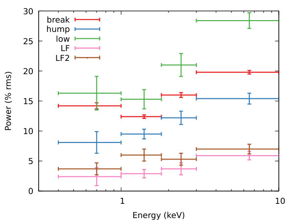 Figure 1
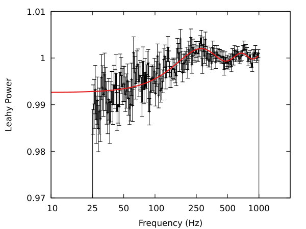 Figure 2
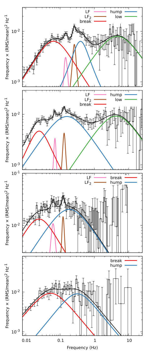 Figure 3
 Figure 4
| Energy | Component | Frequency | Quality | Amplitude | / dof | ||
| (keV) | (Hz) | (% rms) | |||||
| XMM-1 | |||||||
| break | 0\@alignment@align.065(6) | 0.18(6) | 13\@alignment@align.1(6) | ||||
| hump | 0\@alignment@align.40(5) | 0.8(3) | 9\@alignment@align.8(1 | ||||
| ow | 4\@alignment@align.7(9) | 0. (fixed) | 15\@alignment@align.8(8) | 70 / 81 | |||
| LF | 0\@alignment@align.146(5) | 4.2(1.8) | 3\@alignment@align.3(5) | ||||
| 0\@alignment@align.260(7) | 4.3(1.1) | 4\@alignment@align.4(4) | |||||
| break | 0\@alignment@align.046(6) | 0.35(11) | 15\@alignment@align.3(1 | ||||
| hump | 0\@alignment@align.29(2) | 0.26(15) | 23\@alignment@align.4(1 | 104/87 | |||
| ow | 6\@alignment@align.4(1 | 0. (fixed) | 28\@alignment@align.5(1 | ||||
| XMM-2 | |||||||
| break | 0\@alignment@align.0245(18) | 0.52(9) | 9\@alignment@align.4(9) | ||||
| hump | 0\@alignment@align.16(2) | 0. (fixed) | 16\@alignment@align.9(7) | ||||
| ow | 4\@alignment@align.3(7) | 0. (fixed) | 17\@alignment@align.0(8) | 122 / 114 | |||
| LF | 0\@alignment@align.071(2) | 6.4(26) | 2\@alignment@align.8(5) | ||||
| 0\@alignment@align.131(3) | 5.5(1.9) | 3\@alignment@align.4(4) | |||||
| break | 0\@alignment@align.026(3) | 0.32(9) | 18\@alignment@align.7(2 | ||||
| hump | 0\@alignment@align.144(11) | 0.27(13) | 25\@alignment@align.9(2 | 119 / 112 | |||
| ow | 3\@alignment@align.3(6) | 0. (fixed) | 31\@alignment@align.0(1 | ||||
| NuSTAR-1 | |||||||
| break | 0\@alignment@align.024(4) | 0.22(11) | 19\@alignment@align. (2) | ||||
| hump | 0\@alignment@align.19(5) | 0. (fixed) | 25\@alignment@align.2(1 | 94 / 92 | |||
| LF | 0\@alignment@align.062(3) | 3.6(1.7) | 6\@alignment@align.7(1 | ||||
| 0\@alignment@align.123(4) | 6. (3) | 6\@alignment@align.0(1 | |||||
| break | 0\@alignment@align.041(6) | 0. (fixed) | 28\@alignment@align.2(1 | 86 / 77 | |||
| NuSTAR-2 | |||||||
| break | 0\@alignment@align.05(2) | 0.10(20) | 16\@alignment@align. (4) | ||||
| hump | 0\@alignment@align.32(14) | 0. (fixed) | 15\@alignment@align. (5) | 43 / 55 | |||
| break | 0\@alignment@align.054(13) | 0. (fixed) | 15\@alignment@align.2(1 | 59/56 | |||
Peer Reviews
No public reviews on file for this paper yet. If you reviewed it on a platform where reviews are public (OpenReview, ICLR, NeurIPS, ICML), you can paste yours below so the community can read it here.
Videos
No videos yet. Explain this paper in a talk, walkthrough, or lecture? Add one.
The stochastic X-ray variability of the accreting millisecond pulsar MAXI J0911–655
Peter Bult
Astrophysics Science Division, NASA Goddard Space Flight Center, Greenbelt, MD 20771
Abstract
In this work I report on the stochastic X-ray variability of the 340 Hz accreting millisecond pulsar MAXI J0911–655. Analyzing pointed observations of the XMM-Newton and NuSTAR observatories I find that the source shows broad band-limited stochastic variability in the Hz range, with a total fractional variability of rms in the keV energy band, which increases to rms in the keV band. Additionally a pair of harmonically related quasi-periodic oscillations are discovered. The fundamental frequency of this harmonic pair is observed between frequencies of mHz and mHz. Like the band-limited noise, the amplitude of the QPOs show a steep increase as a function of energy, suggesting they share a similar origin, which is likely the inner accretion flow. Based on their energy dependence and their frequency relation with respect to the noise terms, the QPOs are identified as Low-Frequency oscillations, and discussed in terms of Lense-Thirring precession model.
pulsars: general – stars: neutron – X-rays: binaries – individual (MAXI J0911–655)
\AuthorCallLimit
=1
1 Introduction
Accreting Millisecond X-ray Pulsars (AMXPs) are a class of transient neutron star Low-Mass X-ray Binaries (LMXBs) that show coherent pulsations during their outbursts (see Patruno & Watts 2012 for a review). Such pulsations are attributed to magnetically channeled accretion onto the neutron star, so that emission from a localized impact region gives rise to periodic intensity variations at the neutron star spin frequency. By tracking the arrival time of the pulsations the neutron spin frequency and its evolution can be measured. This then gives a direct tool through which the torque mechanisms acting between the star and the surrounding accretion flow may be studied (Psaltis & Chakrabarty, 1999; Bildsten, 1998; Haskell & Patruno, 2011). Additionally, through the timing of the pulsar the binary orbit and evolution may be investigated (Patruno et al., 2012), while careful modeling of the pulse waveform may be used to extract information on otherwise elusive neutron star properties, such as mass, radius, and magnetic field strength (Poutanen & Gierliński, 2003; Leahy et al., 2008; Psaltis et al., 2014).
In addition to coherent pulsations, the X-ray emission from AMXPs also shows rich stochastic variability. Like the broader class of LMXBs (van der Klis, 2006), various timing features may be distinguished in AMXP light curves, including broad band-limited noise terms, and narrow Quasi-Periodic Oscillations (QPOs). Furthermore, the morphology, relative frequencies, and correlations with luminosity or energy spectra that may be observed for these timing features are all largely consistent with those observed in the atoll class of accreting neutron stars (van Straaten et al., 2005).
Atoll type neutron stars are named for the pattern they trace out in the color-color diagram as their luminosity changes (Hasinger & van der Klis, 1989). At high luminosity, their energy spectrum is soft and the bulk of their variability features narrow and concentrated at high frequencies ( Hz). As the luminosity varies, atoll sources trace out a banana shaped pattern in the color-color diagram, which is usually sub-categorized into three source states (upper-, lower- and lower-left banana) depending on the specific morphology of the power spectrum. For lower luminosities, atolls transition into the island state, which is characterized by a harder energy spectrum. Meanwhile, the power spectral features shift to lower frequencies ( Hz), while gaining in both width and amplitude. This trend continues to the lowest observed luminosities where such sources may enter an extreme island state. Here the energy spectrum is dominated by a hard power law, while the bulk power density has shifted down to Hz with only weak QPOs or none at all.
Given that the stochastic timing signatures are generally attributed to the accretion flow, it is of interest to compare the differences and similarity between pulsating and non-pulsating objects as this offers a path to investigating the coupling mechanisms between the neutron star and the accretion flow. In this work I therefore report on the first stochastic X-ray variability study of the accreting millisecond pulsar MAXI J0911–655 (henceforth MAXI J0911) based on observed of the XMM-Newton and NuSTAR observatories.
1.1 MAXI J0911–655
The X-ray transient MAXI J0911, was discovered on February 19th, 2016 (Serino et al., 2016) with the MAXI/GSC. The source was immediately associated with the globular cluster NGC 2808, a position that was later confirmed by Swift/XRT (Kennea et al., 2016) and Chandra (Homan et al., 2016) observations. Subsequent monitoring with INTEGRAL and Swift/XRT has shown that MAXI J0911 has remained active, showing a persistent flux of about mCrab (Ducci et al., 2016). At the time of writing this source is yet to transition into quiescence, placing the duration of the outburst at approximately one year.
The nature of the compact object in MAXI J0911 was settled when its 340 Hz pulsations were discovered by Sanna et al. (2017). Using pointed XMM-Newton and NuSTAR observations, these authors studied the pulsations and showed the AMXP is set in a compact binary with a 44.3 minutes orbital period and a companion star of . The nature of the companion is not definitively constrained, but is likely either a hot, helium white dwarf, or an old brown dwarf. Additionally, they found that the energy spectrum of MAXI J0911 is relatively hard, with a power-law dominating over a weak blackbody component.
2 Data Reduction
2.1 XMM-Newton
In this work I analyze the epic-pn data of two XMM-Newton observations of MAXI J0911. The first observation took place on April 24, 2016 (ObsID 0790181401) and the second on May 22, 2016 (ObsID 0790181501). For both observations the epic-pn camera was operated in timing mode, yielding event list data at a time resolution of 29.56 .
To obtain science grade products, the data was processed with sas version 15.0.0 using the most recent calibration files available. Standard data screening criteria were applied to the data, selecting only those events in the keV energy range with pattern and screening flag. The source data was extracted from a 15 bin wide rectangular region with rawx coordinates . Finally the sas tool barycen was applied to correct the event arrival times to the Solar System barycenter, using the source coordinates of Homan et al. (2016).
The background estimate was obtained similarly, but from a 3 bin wide region with the rawx coordinates . Since this region is smaller than the source extraction region I multiplied the resulting background count rate by a factor of 5 to ensure both source and background rates reflect a comparable effective area.
The source count rates obtained are 40(1) and 35(2) counts/s for the first and second observations, respectively. The associated background count rates are respectively 0.8(4) and 0.4(2) counts/s.
2.2 NuSTAR
NuSTAR observed MAXI J0911 on May 24, 2016 (ObsID 90201024002), and again 180 days later on November 23, 2016 (ObsID 90201042002). The data was processed using the nustardas software pipeline version 1.6.0. This was done separately for each of the two focal plane modules (FPMA and FPMB).
The source events in the keV energy band were extracted from a circular region with a radius that was centered on the image source position. The filtered event arrival times were then corrected to the Solar System barycenter using the barycorr tool, again based on the source coordinates of Homan et al. (2016). The background events were extracted similarly, but with a source region centered in the background field. The resulting source count rates are 2.0(2) counts/s and 3.0(2) counts/s, for the first and second observations, respectively, with a background count rate of 0.01(1) counts/s in both cases.
2.3 Timing Analysis
A stochastic timing analysis is performed on the cleaned and processed X-ray data. First all the arrival times are adjusted for the binary motion of neutron star based on the ephemeris of Sanna et al. (2017). The event lists are then binned into second long light curves using a time resolution of 480 (the length of the time series is adjusted so that the number of time bins is a power of two). For each of these light curves I compute the Fourier transform, from which a Leahy-normalized power spectrum is calculated (Leahy et al., 1983). These power spectra have a frequency resolution of Hz and a limiting Nyquist frequency of Hz. All individual power spectral estimates are averaged per ObsID and corrected for Poisson noise.
For the XMM-Newton data the Poisson noise spectrum is modeled as a constant. That noise power is measured between Hz and Hz, where no signal features are observed, and then subtracted from the averaged power density spectrum.
In the case of the NuSTAR data the instrument deadtime needs to be taken into account, as it has a comparatively long timescale of ms (Harrison et al., 2013). An elegant way of dealing with the NuSTAR deadtime was proposed by Bachetti et al. (2015) and involves computing the complex-valued cross spectrum from the two FPM light curves. The real component of the cross spectrum, also known as the co-spectrum, can then be adopted as an estimator of the source power density spectrum. Because, to good approximation111Deadtime is a multiplicative noise term, so the modulation imposed on the power spectrum is, to some degree, correlated with the spectrum of the signal itself. Correlating a multi-detector system can therefore not completely remove deadtime effects. , the deadtime is independent between detectors, while the signal itself is wholly correlated, this approach effectively filters out any deadtime modulation without the need to model it.
I would point out, however, that the gain achieved through considering the co-spectrum does not come for free. The cost of correlating the two FPM light curves is that the resulting signal-to-noise is lower than what would have been obtained if the two light curves were simply added in the time domain. Specifically, the uncertainties on the co-spectral powers are larger than those obtained from a regular power spectrum by up to a factor of (see appendix A for details).
Given that the observed event rate (0.5 s/count) is much larger than the timescale of the deadtime, the effect of the dead time will be relatively small, and the power spectrum will only be sensitive at comparatively low frequencies. I would therefore argue that in this case it is more appropriate to add the two FPM light curves for the increased sensitivity, rather than correlating them to reduce the deadtime modulation.
The NuSTAR power spectra are constructed by adding the concurrent FPM data. For each light curve the Fourier transforms are computed and normalized, and subsequently averaged in the complex domain. From this averaged Fourier transform a Leahy normalized power spectrum constructed. Note that this power spectrum will have an expected Poisson noise level of (see appendix A). All segments of the ObsID are averaged to a single power spectrum. This power spectrum shows some deadtime modulation, which is modeled heuristically by taking all powers above Hz and fitting the scaled sinc function
[TABLE]
where and are a mean and scale parameter, respectively, and is the characteristic deadtime. For the first NuSTAR observation the best fit gives with parameters , and ms (Figure 1). Below 10 Hz this curve is near constant at a level of , which I adopt as the Poisson noise level and subtract from the data. The second NuSTAR observation has similar results, and differs only in the scale, , so that the Poisson noise level is marginally higher, .
Finally, the Poisson noise corrected averaged power spectra are renormalized to squared fractional rms, and subsequently described in terms of a multi-Lorentzian model (Belloni et al., 2002). Each component, , is a function of Fourier frequency and characterized by three parameters. Here is the characteristic frequency, and the quality factor, where gives the centroid frequency and is the full-width-at-half-maximum. The amplitude of an individual component is expressed in terms of fractional rms, , defined as
[TABLE]
where is the integrated power. A component is considered to be significant if its integrated power has a single trial significance greater than three, that is, if .
3 Results
Because the XMM-Newton and NuSTAR energy bands overlap, the XMM-Newton data is split in a low energy ( keV) and high energy ( keV) band, so that the latter is covered by both observatories, allowing for a direct comparison of their power spectra.
The first XMM-Newton observation (XMM-1) shows significant power in the to Hz frequency range (Figure 2, top panel). The integrated fractional rms amplitude is in the keV band, and increases to in the keV band.
The reference list from the paper itself. Each links out to its DOI / PubMed record.
- 1Altamirano et al. (2012) Altamirano, D., Ingram, A., van der Klis, M., et al. 2012, Ap J, 759, L 20
- 2Altamirano et al. (2008 a) Altamirano, D., van der Klis, M., Méndez, M., et al. 2008 a, Ap J, 685, 436
- 3Altamirano et al. (2005) —. 2005, Ap J, 633, 358
- 4Altamirano et al. (2008 b) Altamirano, D., van der Klis, M., Wijnands, R., & Cumming, A. 2008 b, Ap J, 673, L 35
- 5Altamirano et al. (2011) Altamirano, D., Belloni, T., Linares, M., et al. 2011, Ap J, 742, L 17
- 6Bachetti et al. (2015) Bachetti, M., Harrison, F. A., Cook, R., et al. 2015, Ap J, 800, 109
- 7Belloni et al. (2000) Belloni, T., Klein-Wolt, M., Méndez, M., van der Klis, M., & van Paradijs, J. 2000, A&A, 355, 271
- 8Belloni et al. (2002) Belloni, T., Psaltis, D., & van der Klis, M. 2002, Ap J, 572, 392