Analytic structure of eigenvalues of coupled quantum systems
Carl M. Bender, Alexander Felski, Nima Hassanpour, S. P. Klevansky,, and Alireza Beygi

TL;DR
This paper explores the analytic continuation of coupling constants in quantum systems to understand eigenvalue structures, revealing unconventional states with energies below the ground state, and discusses the physical implications of such continuations.
Contribution
It introduces a method to analyze eigenvalues of coupled quantum systems through complex coupling continuation, highlighting new states and their energetic properties.
Findings
Analytic continuation can lead to states with energies below the original ground state.
Exceptional points in the complex plane influence eigenvalue behavior.
The process requires work, questioning the physical realization of these states.
Abstract
By analytically continuing the coupling constant of a coupled quantum theory, one can, at least in principle, arrive at a state whose energy is lower than the ground state of the theory. The idea is to begin with the uncoupled theory in its ground state, to analytically continue around an exceptional point (square-root singularity) in the complex-coupling-constant plane, and finally to return to the point . In the course of this analytic continuation, the uncoupled theory ends up in an unconventional state whose energy is lower than the original ground state energy. However, it is unclear whether one can use this analytic continuation to extract energy from the conventional vacuum state; this process appears to be exothermic but one must do work to vary the coupling constant .
Click any figure to enlarge with its caption.
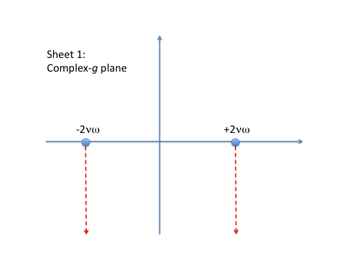 Figure 1
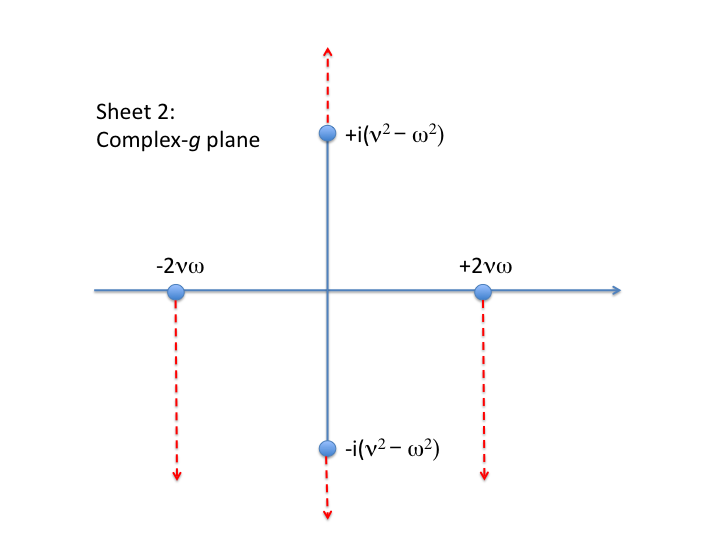 Figure 2
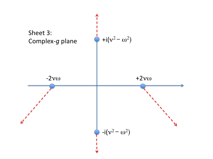 Figure 3
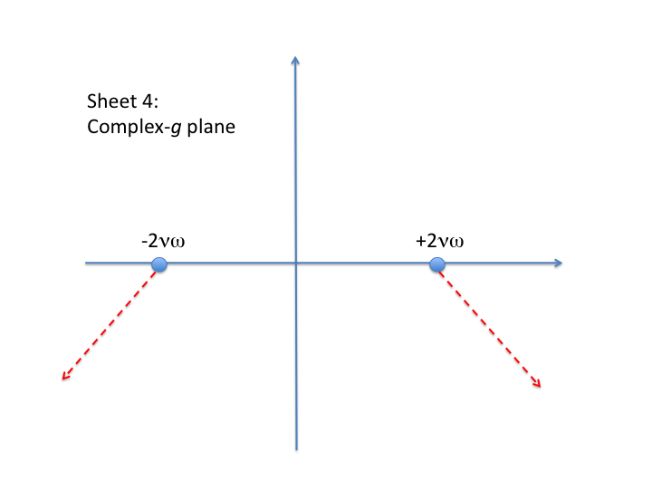 Figure 4
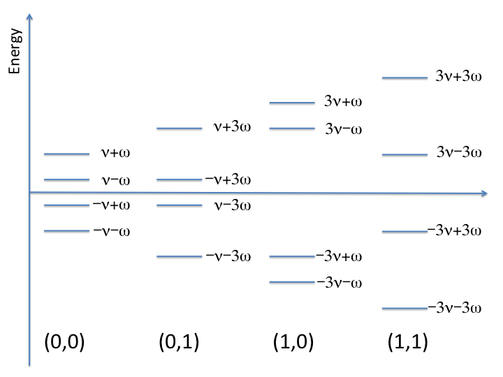 Figure 5
Peer Reviews
No public reviews on file for this paper yet. If you reviewed it on a platform where reviews are public (OpenReview, ICLR, NeurIPS, ICML), you can paste yours below so the community can read it here.
Videos
No videos yet. Explain this paper in a talk, walkthrough, or lecture? Add one.
&pdflatex
Analytic structure of eigenvalues of coupled quantum systems
Carl M. Bender1
Alexander Felski2
Nima Hassanpour1
S. P. Klevansky2,3
Alireza Beygi2
1Department of Physics, Washington University, St. Louis, Missouri 63130, USA
2Institut für Theoretische Physik, Universität Heidelberg, Philosophenweg 12, 69120 Heidelberg, Germany
3Department of Physics, University of the Witwatersrand, Johannesburg, South Africa
Abstract
By analytically continuing the coupling constant of a coupled quantum theory, one can, at least in principle, arrive at a state whose energy is lower than the ground state of the theory. The idea is to begin with the uncoupled theory in its ground state, to analytically continue around an exceptional point (square-root singularity) in the complex-coupling-constant plane, and finally to return to the point . In the course of this analytic continuation, the uncoupled theory ends up in an unconventional state whose energy is lower than the original ground state energy. However, it is unclear whether one can use this analytic continuation to extract energy from the conventional vacuum state; this process appears to be exothermic but one must do work to vary the coupling constant .
pacs:
11.30.Er, 03.65.Db, 11.10.Ef, 03.65.Ge
I Introduction
The analytic structure of eigenvalues of self-coupled systems, such as the quantum anharmonic oscillator, has been studied in great depth. Singularities in the coupling-constant plane have been identified as the cause of the divergence of perturbation theory r1 ; r2 . These singularities are typically square-root branch points and are associated with the phenomenon of level crossing. These singularities are sometimes referred to as exceptional points r3 . Studies of coupling-constant analyticity have revealed a remarkable and generic phenomenon, namely, that the eigenvalues belonging to the spectrum of the Hamiltonian are analytic continuations of one another as functions of the complex coupling constant. Thus, the energy levels of a quantum system, which are discrete when the coupling constant is real and positive, are actually smooth continuations of one another in the complex-coupling-constant plane r4 , and a simple geometric picture of quantization emerges: The discrete eigenvalues of a quantum system are in one-to-one correspondence with the sheets of the Riemann surface. The different energy levels of the Hamiltonian are merely different branches of a multivalued energy function.
While this picture of quantization has emerged from studies of coupling-constant singularities of self-coupled systems, this paper argues that an even more elaborate picture arises from studies of coupled quantum systems. Consider, for example, the simple case of two coupled quantum harmonic oscillators, one having natural frequency and the other having natural frequency . For definiteness, we assume that . The Hamiltonian for such a system has the form
[TABLE]
where is the coupling parameter. For sufficiently large the eigenvalues of become singular. To demonstrate this we rewrite the potential as
[TABLE]
We see immediately that on the line in the plane becomes unbounded below if . Thus, while the potential has a positive discrete spectrum when the coupling constant lies in the range
[TABLE]
we expect there to be singular points at in the coupling-constant plane. This result raises the question, What is the nature of the singular points at ?
Coupled-oscillator models have been studied in great detail in many papers r5 ; r6 ; r7 ; r8 ; r9 ; r10 ; r11 and in particular for oscillator models of the type in (1). The presence of singularities at was noted in r6 ; however, the nature of singularities and the Riemann sheet structure was not identified in any of these papers.
In this paper we show that the Riemann surface for the coupled-oscillator Hamiltonian (1) consists of four sheets. The singularities at are square-root singularities, like the exceptional-point singularities of self-coupled oscillators. However, if we cross either of the square-root branch cuts, we enter a second sheet of the Riemann surface on which two new square-root branch points appear. These new branch points are located at . If we cross either of the branch cuts emanating from these new branch points, we enter a third sheet of the Riemann surface where there are yet another pair of square-root singularities at , unconnected with the singularities on sheets one and two. Crossing either of the branch cuts emanating from these singularities at takes us to a fourth sheet of the Riemann surface. Not all energy levels of the coupled harmonic oscillator mix among themselves as varies on this four-sheeted Riemann surface. Rather, each energy level belongs to a quartet of energies that are analytic continuations of one another. We find that the four sheets of the Riemann surface correspond to four distinct spectral phases of the coupled oscillator system (1).
We give a detailed description of these spectral phases in Sec. II. We explain below how such spectral phases arise. Let us consider a single harmonic oscillator, whose dynamics are defined by the Hamiltonian
[TABLE]
This simple quantum system actually has two spectral phases characterized by two distinct spectra. To understand why, we assume that is a positive parameter and we note that the th eigenvalue , which is defined by the eigenvalue problem
[TABLE]
is given by
[TABLE]
In r12 it was observed that if we analytically continue in a semicircle in the complex- plane, that is, if we let ( real) and allow to run from [math] to , the eigenvalues change sign even though the Hamiltonian remains unchanged. By this analytic continuation we reach a new phase of the harmonic oscillator whose spectrum is negative and unbounded below. Thus, the Hamiltonian (4) of the harmonic oscillator has two distinct and independent real spectra that are related by analytic continuation in the natural frequency of the oscillator.
How can one Hamiltonian (4) have two different spectra? The answer to this question is that the positive spectrum is obtained by imposing the boundary conditions in (5) in a pair of Stokes wedges r13 ; r14 ; r15 ; r4 centered about the positive-real- and negative-real- axes. We refer to the positive spectrum as the conventional one. These wedges have angular opening . The negative spectrum is defined by imposing the boundary conditions in a pair of Stokes wedges containing and centered about the upper and lower imaginary- axes. We refer to the negative spectrum as the unconventional spectrum of the harmonic oscillator. These Stokes wedges also have angular opening of . To understand the configuration of the wedges we examine the WKB geometrical-optics approximation r4
[TABLE]
to the solutions of the harmonic-oscillator eigenvalue equation (4). On the basis of (6) we can see that the wedges in which the eigenfunctions vanish rotate clockwise through an angle of as rotates anticlockwise through an angle of . Thus, these two phases are analytic continuations of one another and are analytically connected by rotations in the complex-frequency plane.
A principal result of this paper is that, if we analytically continue the physical system consisting of two coupled harmonic oscillators described by the Hamiltonian in (1) in the coupling constant parameter , we obtain all four possibilities for the phases of the two oscillators in which each oscillator is in a conventional or an unconventional phase. Thus, all four phases are analytically connected on the Riemann surface of the complex coupling constant , even though the frequencies and are held fixed and positive.
In Sec. II we construct analytically the four-sheeted Riemann surface for the coupled harmonic oscillator model (1). In Sec. III we examine the Riemann surface defined by the partition function for some zero-dimensional quantum field theories. In general, the number of sheets in the complex Riemann surface for these theories is smaller than the number of sheets for the corresponding quantum-mechanical problem. For example, for the zero-dimensional quantum field theory that is analogous to the quantum-mechanical oscillator model of (1), the Riemann surface only has two sheets and not four sheets. For a coupled pair of sextic models, the Riemann surface has six sheets, indicating that this theory has six different phases. Section IV gives some brief concluding remarks.
II Energy Levels of the Coupled Harmonic Oscillator
In this section we examine the analytic structure of the eigenvalues of the coupled harmonic oscillator Hamiltonian (1). We begin by examining the ground state, whose eigenfunction has the general form
[TABLE]
where , , and are constants to be determined. We substitute (7) into the eigenvalue equation , which has the explicit form
[TABLE]
We then equate the coefficients of , , , and and obtain the four equations
[TABLE]
Subtracting the first equation from the second and combining the result with the third and fourth equations allows us to calculate , , and , which we then eliminate in favor of a single quartic polynomial equation for the eigenvalue E:
[TABLE]
The solution to this equation involves nested square roots,
[TABLE]
and from this equation we see that is a four-valued function of the coupling constant .
Let us make a grand tour of the Riemann surface on which is defined. We begin on Sheet 1, where both square-root functions are real and positive when their arguments are real and positive. There are two obvious square-root branch points (zeros of the inner square root) and these are located at . Square-root branch cuts emerge from each of these branch points and, as shown on Fig. 1, we have chosen to draw these branch cuts as vertical lines going downward. On Sheet 1
[TABLE]
and because we assume that and are real and positive we see that both oscillators are in their conventional ground states.
There are no other singularities on Sheet 1 that allow us to change the sign of the outer square root. This is because at such a singular point the argument of the outer square root function would have to vanish:
[TABLE]
The solution of this equation is obtained by squaring :
[TABLE]
so is positive. The solution in (15) is spurious because both terms in (14) are positive.
If we analytically continue through either of the branch cuts on Sheet 1, we arrive on Sheet 2, where the inner square root changes sign. Therefore, on this sheet
[TABLE]
assuming that . Thus, the oscillator is in its conventional ground state but the oscillator is in its unconventional ground state. Because the inner square root returns negative values when its argument is positive, the solution for in (15) is not spurious. Therefore, there are new branch cuts associated with the sign change of the outer square root; these branch cuts emanate from branch points located at
[TABLE]
All four branch cuts on Sheet 2 are shown on Fig. 2. If we now pass through a branch cut emanating from , we return to Sheet 1 but if we pass through a branch cut emanating from either branch point in (17), we enter Sheet 3.
On Sheet 3 there are two pairs of square-root branch cuts. The branch points on the imaginary axis coincide with those on Sheet 2. However, there is a new pair of branch points on the real axis at . Although these branch points appear at the same locations as on Sheets 1 and 2, they are unrelated to those branch points. We show this explicitly in Fig. 3 by drawing the associated branch cuts differently. On this sheet both the inner and outer square-root functions in (12) are negative and
[TABLE]
when is positive. Now the oscillator is in an unconventional ground state and the oscillator is in a conventional ground state.
If we now pass through a branch cut emanating from (17), we return from Sheet 3 to Sheet 2. However, if pass through a branch cut emanating from , we enter Sheet 4. On this sheet there are only two branch points, which are located at (see Fig. 4). On Sheet 4
[TABLE]
Both oscillators are now in unconventional ground states.
To summarize, Figs. 1-4 describe each of the four branches of the function in (12). On these four branches takes the values given in (13), (16), (18), and (19). From these four values of we infer that by analytically continuing the two-coupled-oscillator system in (1) through the entire Riemann surface we access both phases, conventional and unconventional, of both oscillators, even though the two frequency parameters and are held fixed.
The four-fold structure of the ground-state energy is repeated for all of the energy levels. To verify this, we construct the eigenfunctions associated with the other energy levels of the theory. These eigenfunctions consist of the exponential in (7) multiplied by a polynomial . If has the form
[TABLE]
the eigenvalue equation (8) leads to the three coupled equations (9) together with four alternatives for :
[TABLE]
For the quartet of ground state energy levels described above, , , so that . We assign the label to this quartet because it reduces to the (conventional and unconventional) ground states of the and oscillators when and . We use the designation for the quartet , for the quartet , and for the quartet that give rise to spectra in the decoupling limit , . In this limit, it follows again that and , leading to four quartets with the additional three spectra arising from (22) for (1,0) when , (23) for (0,1) when and (24) for (1,1) when . These four quartets are illustrated in Fig. 5 for the case and . We emphasize that the energy levels of different quartets are not analytic continuations of one another but the elements of each quartet are analytic continuations of one another and branches of a four-valued function defined on exactly the same the Riemann surface pictured in Figs. 1-4.
III Partition functions for zero-dimensional field theories
III.1 Interacting quadratic field theory
Let us examine the zero-dimensional field-theoretic equivalent of the Hamiltonian (1). The partition function for this field theory is given by the integral
[TABLE]
where both integration paths run from to . We can evaluate the integral exactly by rearranging the terms in the exponential as we did in (2):
[TABLE]
Simple transformations then reduce this to a product of two gaussian integrals,
[TABLE]
which evaluate to
[TABLE]
This partition function is a double-valued function of and is defined on a two-sheeted Riemann surface. Like the coupled harmonic oscillator discussed in Sec. II the square-root singularities are located at . However, unlike the case of the coupled harmonic oscillator, the Riemann surface has two sheets and not four; these sheets correspond to the two possible signs of and these two sheets correspond to the analogs of the conventional-conventional theory and the unconventional-unconventional theory. (To obtain the unconventional-unconventional theory from the conventional-conventional theory we replace by and by and this changes the sign of the partition function.) There is no analytic continuation to the partition function for a mixed unconventional-conventional theory. This is because the path of integration is included with the integral that defines the partition function. Given an eigenvalue differential equation we are free to choose the boundary conditions (we can require that the eigenfunctions vanish as or as ) but there is no such freedom in the case of an integral. To obtain other phases we would have to change the path of integration in the definition of the partition function.
We can generalize this calculation by including in the partition function external fields and coupled to the and fields:
[TABLE]
Evaluating this integral by following the same procedure as above, we now find a more elaborate singularity structure,
[TABLE]
which is again defined on a two-sheeted Riemann surface but in addition has essential singularities at the square-root branch points. Consequently, all of the Green’s functions, which are obtained by taking derivatives with respect to the external sources, have increasingly stronger singularities at .
III.2 Interacting sextic field theory
A higher-power selfinteracting field theory that possesses a conventional real spectrum and in addition possesses a real -symmetric spectrum has a sextic interaction of the form . We thus examine a field theory that describes the coupling of two sextic oscillators and we choose a symmetric form for the coupling. The partition function for the zero-dimensional version of this coupled quantum field theory is
[TABLE]
This sextic theory is more difficult to examine analytically. We begin by expanding the coupling term as a series in powers of :
[TABLE]
Since the and integrals run from to , only even values of contribute to the partition function. When is even, we have
[TABLE]
but if is odd, the integral vanishes. Thus, we make the replacement and re-express the partition function as a sum over :
[TABLE]
This sum is a hypergeometric series:
[TABLE]
In general, the hypergeometric series has a radius of convergence of 1. (This is easy to verify by using the Stirling approximation for the Gamma function.) This implies that has a singularity on the circle .
It is important to identify the precise location and nature of this singularity. To do so we use the linear transformation formula r16
[TABLE]
This transformation makes the singularity explicit because the hypergeometric function is analytic in the unit circle. Applying this transformation gives
[TABLE]
from which we conclude that is defined on a six-sheeted Riemann surface and that the branch points on all six sheets of the Riemann surface are located at , which corresponds with the singularities of the coupled harmonic oscillator model at with .
More generally, we can examine the Green’s functions of the theory, which are defined as integrals of the form
[TABLE]
where and are integers. It is necessary that is even for the Green’s function to be nonvanishing. Following the same analysis as above, we find that all Green’s functions are defined on a six-sheeted Riemann surface and that the singularity in the complex- plane has the form
[TABLE]
Thus, like the Green’s functions for the coupled harmonic oscillator, we see that the singularity becomes stronger with increasing and , but the Green’s functions are always six-valued functions of .
IV Conclusions
We have shown that a coupled quantum theory has a rich analytic structure as a function of the coupling constant. By analytically continuing in the coupling constant we can obtain different spectral phases of the uncoupled theory. Indeed, if we think of the coupling constant as an external classical source, then by varying this external source in a closed loop in the complex-coupling-constant plane we can even imagine extracting energy from the conventional ground state of such a theory, at least in principle. For example, we can begin with the uncoupled harmonic-oscillator system (1) in its conventional ground state (13). We then turn on the source , smoothly and continuously vary , and finally turn off again when the system is in the unconventional ground state (19). Such a process appears to be exothermic because it extracts an amount of energy equal to . However, varying the coupling constant may require that we do work on the system. Until now, it is not clear what it means to vary a coupling constant through complex values. However, remarkable progress on this is currently being made from an experimental point of view. It is experimentally possible to vary the parameters of a system and by doing so to analytically continue from one energy state to another. Such a process has actually been achieved in the laboratory by smoothly varying the parameters of a microwave cavity r17 and, in doing so, going continuously from one frequency mode to another. More recently, experiments have been performed in which an exceptional point is dynamically encircled r18 ; r19 . That is, a combination of physical parameters is varied in real time, and the system response is measured, allowing one to access different Riemann surfaces. While r19 emphasizes robust switching, r18 concerns itself with energy transfer between different states of a system, such as has been considered here in our illustrative prototypical system. An experimental approach, whether optomechanical or using micro, light, acoustic, or matter waves, may in the future yield experimental verification of the analytic continuation discussed in this work.
Finally, these studies have been performed for linear couplings between the oscillators, which led to the four-fold structure shown here. It is to be expected that other types of couplings lead to different, possibly more complicated Riemann surfaces.
Acknowledgements.
CMB thanks the Graduate School of Heidelberg University for their hospitality.
The reference list from the paper itself. Each links out to its DOI / PubMed record.
- 1(1) C. M. Bender and T. T. Wu, Phys. Rev. Lett. 21 , 406 (1968).
- 2(2) C. M. Bender and T. T. Wu, Phys. Rev. 184 , 1231 (1969).
- 3(3) W. D. Heiss, J. Phys. A: Math. Theor. 45 , 444016 (2012).
- 4(4) C. M. Bender and S. A. Orszag, Advanced Mathematical Methods for Scientists and Engineers (Mc Graw-Hill, New York, 1976).
- 5(5) H. Bateman, Phys. Rev. 38 , 815 (1931).
- 6(6) C. M. Bender and H. F. Jones, J. Phys. A: Math. Theor. 41 , 244006 (2008).
- 7(7) I. L. Aleiner, B. L. Altshuler, and Y. G. Rubo, Phys. Rev. B 85 , 121301 (2012).
- 8(8) C. M. Bender, M. Gianfreda, B. Peng, S. K. Ozdemir, and L. Yang, Phys. Rev. A 88 , 062111 (2013).