Trading Lightly: Cross-Impact and Optimal Portfolio Execution
Iacopo Mastromatteo, Michael Benzaquen, Zoltan Eisler, Jean-Philippe, Bouchaud

TL;DR
This paper extends the linear propagator model to multiple correlated instruments to accurately estimate impact costs, emphasizing the importance of considering cross-impact effects for optimal execution strategies.
Contribution
It introduces a multivariate impact cost model that accounts for cross-impact effects, improving the accuracy of liquidity estimation and execution strategies.
Findings
Neglecting cross-impact leads to suboptimal execution.
Synchronizing execution of correlated contracts improves performance.
The model is calibrated on US stock data and is arbitrage-free.
Abstract
We model the impact costs of a strategy that trades a basket of correlated instruments, by extending to the multivariate case the linear propagator model previously used for single instruments. Our specification allows us to calibrate a cost model that is free of arbitrage and price manipulation. We illustrate our results using a pool of US stocks and show that neglecting cross-impact effects leads to an incorrect estimation of the liquidity and suboptimal execution strategies. We show in particular the importance of synchronizing the execution of correlated contracts.
Click any figure to enlarge with its caption.
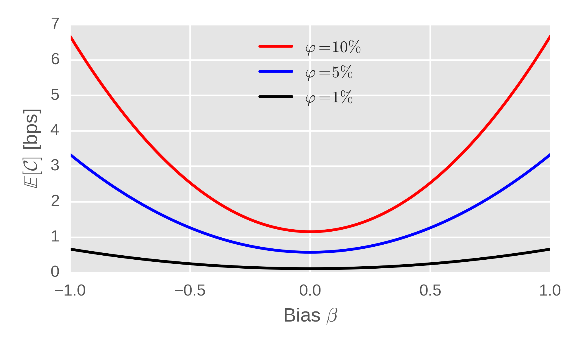 Figure 1
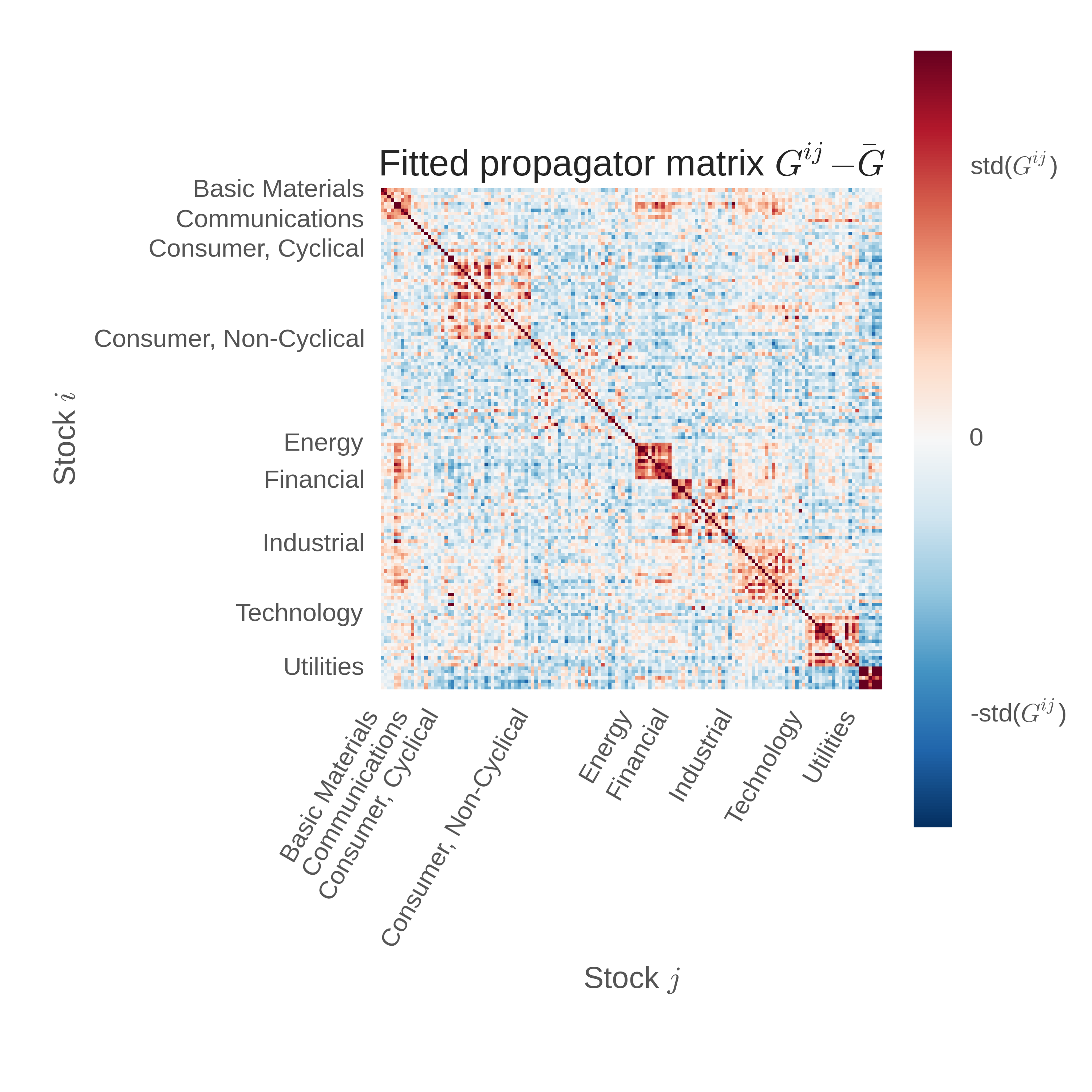 Figure 2
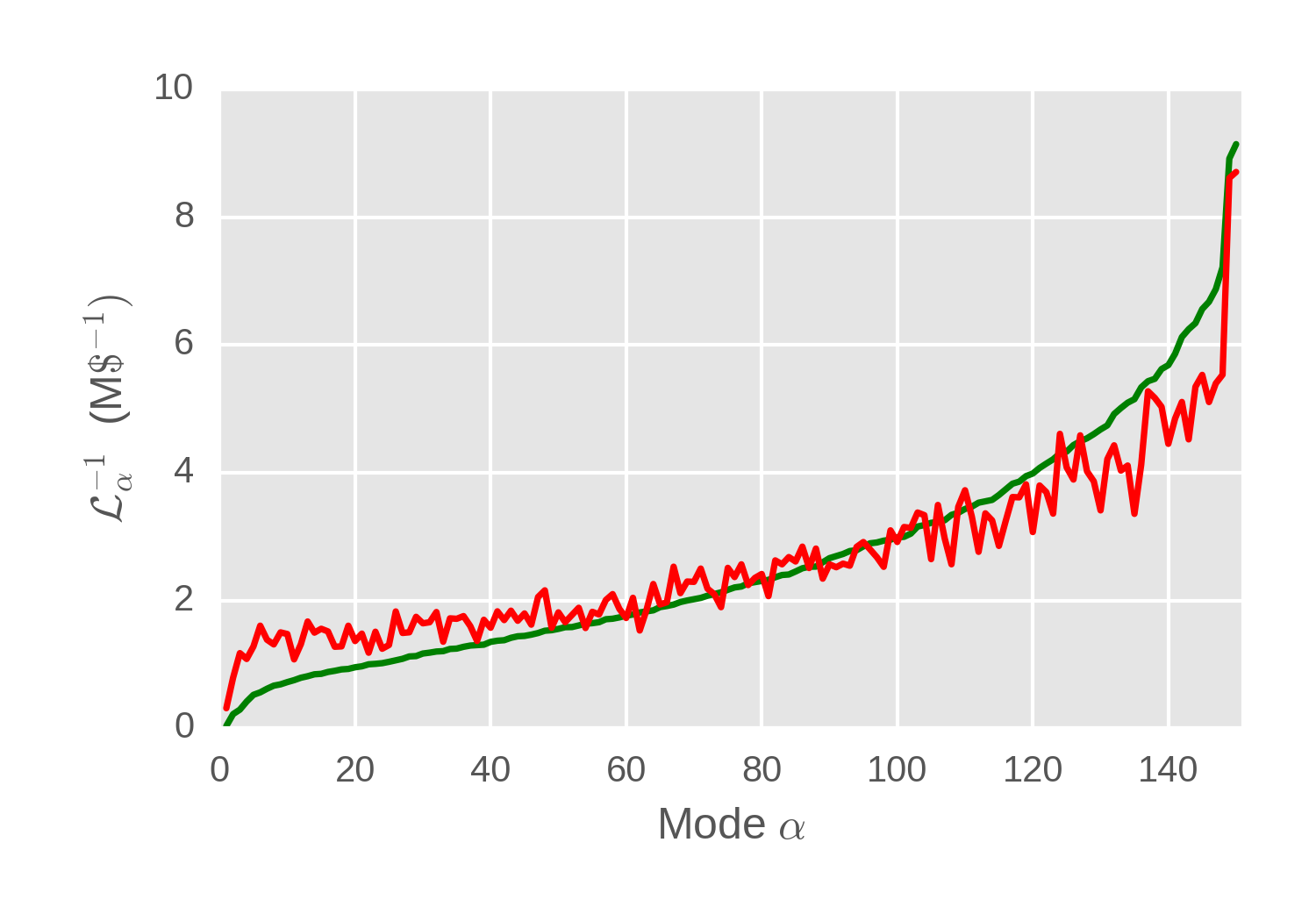 Figure 3
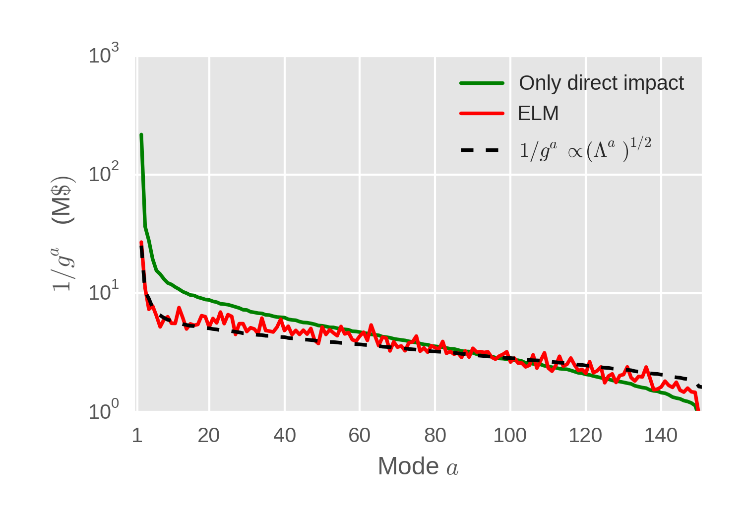 Figure 4
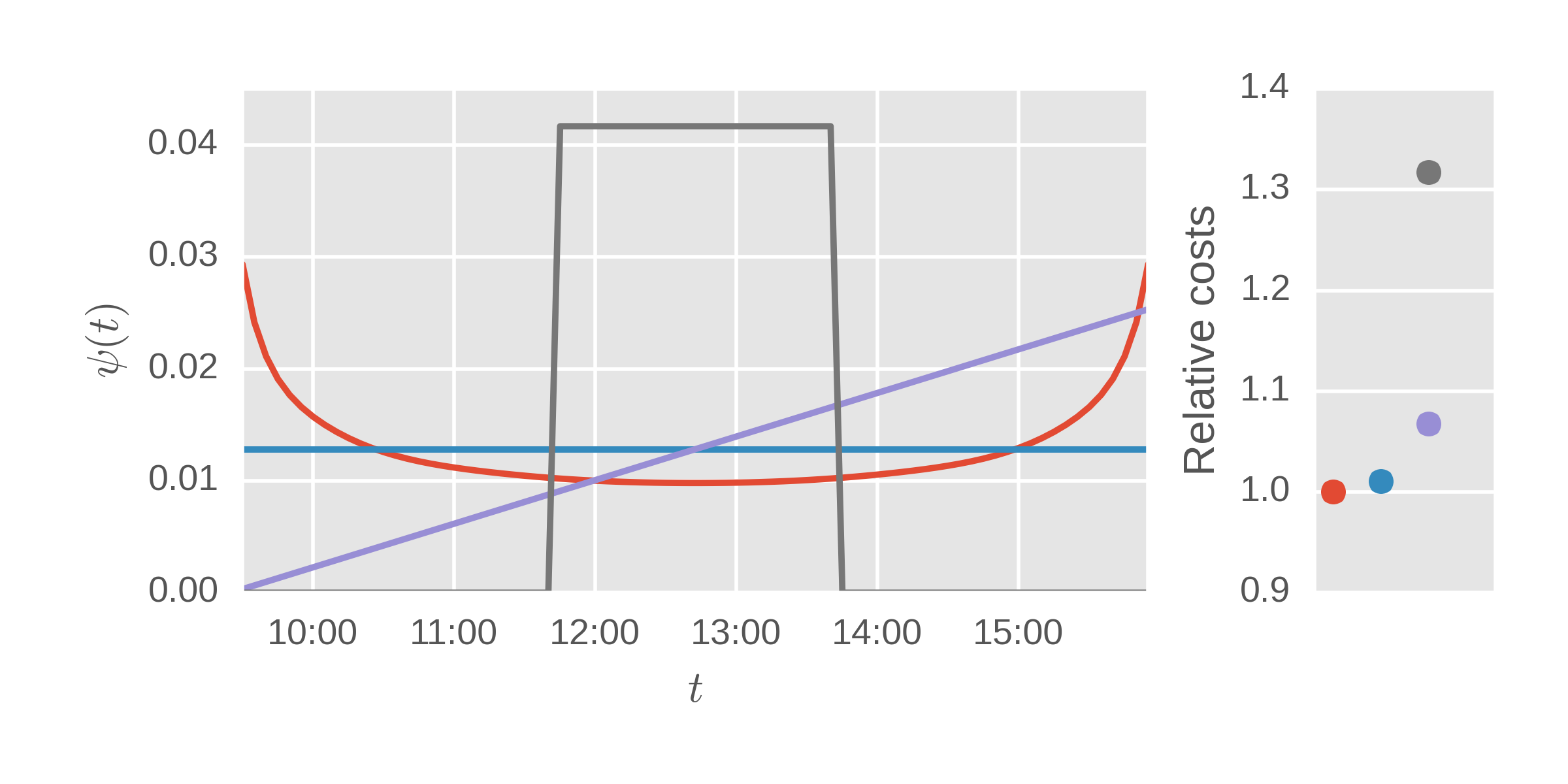 Figure 5
Peer Reviews
No public reviews on file for this paper yet. If you reviewed it on a platform where reviews are public (OpenReview, ICLR, NeurIPS, ICML), you can paste yours below so the community can read it here.
Videos
No videos yet. Explain this paper in a talk, walkthrough, or lecture? Add one.
Trading Lightly:
Cross-Impact and Optimal Portfolio Execution
I Mastromatteo
Capital Fund Management, 23 rue de l’Université, 75007 Paris
M Benzaquen
Capital Fund Management, 23 rue de l’Université, 75007 Paris
Ladhyx, UMR CNRS 7646, École Polytechnique, 91128 Palaiseau Cedex, France
Z Eisler
Capital Fund Management, 23 rue de l’Université, 75007 Paris
J-P Bouchaud
Capital Fund Management, 23 rue de l’Université, 75007 Paris
Abstract
We model the impact costs of a strategy that trades a basket of correlated instruments, by extending to the multivariate case the linear propagator model previously used for single instruments. Our specification allows us to calibrate a cost model that is free of arbitrage and price manipulation. We illustrate our results using a pool of US stocks and show that neglecting cross-impact effects leads to an incorrect estimation of the liquidity and suboptimal execution strategies. We show in particular the importance of synchronizing the execution of correlated contracts.
Executing trading decisions in real markets is a difficult business. Moving around substantial amounts is often foiled by the lack of liquidity. When orders exceed the small volumes typically available at the best bid or ask in lit order books, the incurred slippage costs rapidly become detrimental to the trading strategy. Accurately predicting these trading costs is quite a non-trivial exercise, and one must often resort to statistical models. Most of the complexity of such models arises from price impact, i.e. the fact that trades tend to move market prices in their own direction. This effect has recently triggered a large amount of theoretical activity, due to its direct relation to supply and demand, and also because of the abundantly available data on financial transactions. As alluded to above, this interest is not purely academic, since reliable estimates of trading costs are crucial in order to judge whether one should enter into a position and – if the cost model is accurate enough – to attempt to optimize the execution strategy. For example, splitting large orders into a stream of smaller ones over time is one of the universally accepted ways to mitigate transaction cost. However, as always, the devil is in the details, and the precise nature and time scheduling of the orders can make a large difference to the final result.
Optimal execution problems are widespread in the literature and many different formulas and techniques have been developed to solve them. However, most of these problems are restricted to single asset execution. Recently in Benzaquen et al. (2017) we have shown that even a simple linear model of cross-asset price impact leads to a very rich phenomenology, in line with the results of Wang et al. (2015); Wang and Guhr (2016). In the present paper we provide a practical recipe to optimize the execution of a portfolio of trades, taking into account the cross-impact on the different underlying products within the multivariate framework of Schied et al. (2010). We will show that proper synchronization of the legs of the execution schedule is very important. To quantify the slippage incurred by the strategy we introduce the EigenLiquidity Model (ELM). The model is directly related to statistical risk factors which have been used for portfolio risk management for several decades. Based on a Principal Component Analysis of the correlation matrix, which provides a practical method to quantify the amount of different kinds of market risk (long the market, sectorial, etc.) one can trade while staying within a prescribed budget of transaction cost.
1 A quadratic cost model for a single stock
To set the stage, let us first discuss the execution of a single company’s stock over a trading day that starts at time and lasts until . The total volume we have to trade is shares, which is obtained over the day by a continuous execution schedule whose local speed is , normalized as . If we were to hold this position, our expected risk, defined as the standard deviation of the daily PnL, would be , where is the daily volatility of the stock, expressed in dollars. For convenience let us define the trading speed in risk units as , and the total risk exchanged over the day as , which naturally equals .
A standard model for estimating the cost incurred when trading a certain volume has first been introduced by Almgren and Chriss (2001). We will consider their framework in a setting in which the trader is risk-neutral, and impact is linear and transient (Gatheral et al., 2012; Gatheral and Schied, 2013; Busseti and Lillo, 2012; Alfonsi and Schied, 2013). This allows one to express the trading costs as
[TABLE]
where is an impact kernel (Bouchaud et al., 2004), which quantifies the effect of a small trade on the price at a later time . is typically a decreasing function, dropping from a maximum value obtained at to zero after a slow decay. Consistently with the results of Bouchaud et al. (2004), it can be written as , with
[TABLE]
has units of 1/\$$, and its inverse corresponds to the amount of risk one would have to trade, in the absence of decay, to move the stock’s price by its typical daily volatility \sigma$.
In spite of some limitations (e.g. impact is empirically found to be a sub-linear function of volume), the model above provides a reasonable estimation of trading costs for large trades and it is able to capture the main effects of the trade schedule on costs (Gatheral et al., 2012; Gatheral and Schied, 2013; Alfonsi and Schied, 2013). Extensions of this model to account for risk-aversion have been considered in (Almgren and Chriss, 2001; Obizhaeva and Wang, 2013; Curato et al., 2016), and for bid-ask spread effects in (Obizhaeva and Wang, 2013; Curato et al., 2016).
2 Optimal trading of a single stock
Optimal trading schedules under the cost function (1) for a fixed total volume to execute have been extensively investigated in the finance literature (Gatheral et al., 2012; Gatheral and Schied, 2013; Alfonsi and Schied, 2013; Obizhaeva and Wang, 2013; Busseti and Lillo, 2012). The trajectory of minimum cost can be written as , where and can be determined by solving a linear integral equation (Gatheral et al., 2012). This yields the well-known symmetric bucket shape solution for that is depicted in Figure 1 (red curve).
The optimal solution indicates that after an initial period of faster trading, one should slow down the execution in order to limit the extra cost due the impact of one’s own trades, and then accelerate again the trading near the market close. Since trading does not extend beyond that point, strongly impacting the price in this final period does not penalize any further executions. As an example, the optimal policy is about 30% less expensive than a localized flat two-hour execution, and approximately 7% cheaper than the linear trading profile represented in Figure 1.
The temporal shape of the impact kernel precludes price manipulation, meaning that no round-trip trajectory is capable of making money on average (Gatheral, 2010; Alfonsi and Schied, 2010; Alfonsi et al., 2012).
3 A quadratic cost model for portfolios
The problem of optimal execution across multiple instruments has been first considered in Schied et al. (2010); Kratz and Schöneborn (2014); Schöneborn (2016), whereas the cost model defined above has been generalized to the multivariate case in Alfonsi et al. (2016) (see also Schneider and Lillo (2016) for a non-linear generalization). Within that framework, our definition of risk above is readily extended to a portfolio of multiple stocks with risk positions as
[TABLE]
where the correlation matrix is constructed from the price covariance matrix through
[TABLE]
The daily volatilities are generalized to .
Similarly, Eq. (1) can be extended to this setting as
[TABLE]
The interpretation of the matrix elements of is as before: After trading dollars of risk on the contract at time , we expect the price of contract to change by units of its daily dollar volatility . The terms with correspond to direct price impact, which was already described by earlier models where each stock is independent. In addition, the new terms with describe cross-impact between stocks which, as it was shown by Benzaquen et al. (2017), is a highly relevant effect since it explains an important fraction of the cross-correlation between stocks, a feature that we will use below.
Benzaquen et al. (2017) have further found that within a good degree of approximation, one can write the kernel in the factorized form , with given by Eq. (2), and denote respectively the symmetric and antisymmetric part of . Schneider and Lillo (2016) have shown that when the antisymmetric part of the propagator is large, then price manipulation is possible, leading to an ill-defined cost of optimal strategies. Since empirically is small, we set it to zero so that the cost associated with the execution of a portfolio of trades reads:
[TABLE]
The condition of symmetry for is not the only one required in order not to have price manipulation. In fact, formula (6) is free of price manipulation if and only if is positive semidefinite. This amounts to saying that buying a portfolio always pushes its price up and vice versa, regardless of its composition, resulting in an impact cost that is always greater or equal to zero independently of the portfolio that is actually traded.
4 The EigenLiquidity Model
In principle, can be determined using simultaneous Trades and Quotes data for the corresponding pool of stocks. However, the empirical impact matrix is in general extremely noisy, so some cleaning scheme is necessary. By leveraging the empirical results of Benzaquen et al. (2017) (see Fig.7 therein), showing that the structure of the impact matrix is in a suitable statistical sense “close” to the one of the correlation matrix, we make the assumption that the impact matrix has the same set of eigenvectors as those of the correlation matrix . Intuitively, the eigenvectors of correspond to portfolios with uncorrelated returns. Our assumption means, quite naturally, that trading one of these portfolios will only impact (to first approximation) the returns of that portfolio, but not of any other orthogonal one. Besides being an empirically reasonable cleaning scheme for , this choice is motivated by the results illustrated in this section, showing that it leads to a cost function that satisfy three fundamental consistency requirements: symmetry, positive semi-definiteness and fragmentation invariance.
More precisely, one can write
[TABLE]
where is an orthogonal matrix of eigenvectors and is a diagonal matrix of non-negative eigenvalues. Our assumption is that the matrix has the following structure:
[TABLE]
where is a diagonal matrix, and .
An important property of this decomposition is that it leads to a fragmentation invariant cost formula in the following sense: When trading two completely correlated products and (i.e., when ), the impact of a trading trajectory does not depend on how the volume is split between the two instruments. More formally, a fragmentation invariant cost is left unchanged under the transformation
[TABLE]
where is completely arbitrary. Intuitively, Eq. (8) fulfills this property because of the factor multiplying . If instruments and are completely correlated, then the relative mode “rel” is an eigenvector of zero risk, with . When used for estimating the cost of an execution trajectory , Eq. (8) will single out such relative modes through the projection , and it will weight them by the corresponding risk which is zero.
The impact model (8) will be called the EigenLiquidity Model (ELM). It can be seen as the most natural choice among all the models implementing fragmentation invariance. In fact, it continuously interpolates between small risk modes (that are thus expected to be characterized by small impact) and large risk modes (for which impact costs can be substantial).
Empirically, Eq. (8) has been shown to hold to a good degree of approximation in Benzaquen et al. (2017). On the other hand, the condition of positive semi-definiteness of , i.e. , , is not guaranteed from Eq. (8) and thus should be checked on empirical data. This is what we display in Figure 3 using real data, confirming that all the ’s are actually strictly positive. The quantity has the natural interpretation of a liquidity per mode. It expresses the amount of daily risk in dollars that one can trade on the eigen-portfolio to move its price by its daily volatility .
5 Optimal trading of portfolios
Under the ELM, the impact cost of any schedule admits an interpretation in terms of the modes of the correlation matrix of normalized returns through the decomposition
[TABLE]
where . We have also introduced the notation
[TABLE]
denoting the projection of the executed volumes on a set of uncorrelated, unit risk eigen-portfolios .
The notion of eigen-portfolios is very useful for intuitively characterizing the cost formula (11). The name comes from the fact that these portfolios are not only uncorrelated and unit-risk (i.e., ), but furthermore trading an amount of the basket according to the weights given by has no impact on the total value of the basket and vice versa (i.e., ). This is precisely the intuition behind our central assumption, Eq. (8).
This construction implies that the cost can be calculated by first projecting the strategy on the portfolios via Eq. (12) and then by taking a sum of an impact cost per mode with a weighting factor given by such projections.
Eq. (11) also shows clearly that the positivity of the matrix and the kernel makes the optimization problem convex, which always has a unique solution. The optimum under the terminal constraint is necessarily achieved under a synchronous execution schedule where at any given point in time all stocks are traded with the same time profile, i.e., , resembling the case without cross-impact.
Intuitively, an asynchronous execution strategy can be seen in the mode space as the optimal one above, plus a round-trip along some of these modes. The convexity of the cost function (6) implies that round-trips always increase execution costs, so they should be avoided.111One may compare this with a related discussion by Wang (2017) investigating the case of round-trips on two stocks. Hence, synchronicity is a general consequence of the convexity of the problem, together with the homogeneity of the decay kernels for different instruments.
A toy example to explain the implications of the formalism is given in Box 5.
6 Applications to real data
We have fitted the ELM to a pool of 150 US stocks in 2012, following the procedure described in detail in Box 5. In Benzaquen et al. (2017) for the time decay of impact we find , and seconds.
A visual representation of the impact matrix is shown in Figure 2. The inhomogeneity of captures the sectorial structure of the market, encoding the specific dependence of stock on its sector and/or its most correlated stocks .
The main difference of our ELM and a model without cross-impact is that the impact costs of a large buy program can no longer be reduced as effectively by spreading the orders across multiple correlated instruments. The impact kernel diffuses the interaction across markets and sectors through the modes. The transaction cost of trading dollars of risk in the mode is equal to dollars. Figure 3 shows the inverse of the eigenvalues , this is about 30M dollars of risk on the most liquid mode. Most of the cross-interaction between stocks is captured by this market mode, which accounts for the fact that when buying a dollar of risk of a stock picked at random in our pool, the other stocks in the pool rise on average by times their daily volatility, where is the average of the off-diagonal elements of . Smaller risk modes may be up to 30 times less liquid. Empirically, the liquidity per mode is well fitted by , see Figure 3. This finding is consistent with the assumption of fragmentation invariance, which implicitly requires the parameters when (see Box 5).
In order to illustrate the relevance of these findings when executing a portfolio of trades, let us study numerically a toy daily execution problem of a trader who has target volumes corresponding to a fraction 1%,5%, 10% of the daily liquidity of each of US stocks. We assume that the trader uses the optimal, synchronous policy derived above: .
To explore a variety of trading styles, we set the sign ( for buy, for sell) of the orders from biased coin tosses. We vary the bias parameter in the interval . The interpretation of this construction for or is very simple:
- •
For , the order is a long or short directional one, and is strongly exposed to the market mode of risk.
- •
For , the strategy is neutral, and its exposition to the market mode is therefore limited.
The average cost under such an execution policy can be expressed analytically, allowing to obtain a relation between the cost and :
[TABLE]
where denotes average dollar risk exchanged by the market on the different stocks.
Comparing Eq. (12) between the above special cases, one can see that the dollar cost is higher for than for by a factor that can be estimated on the basis of Eq. (12) to roughly be . This makes sense, as this is the ratio of the top eigenvalue of , expressing the cost of trading the market directionally, versus the average of all eigenvalues selecting the direct impact contribution in the left term of Eq. (12). Figure 4 shows the full evolution of this ratio as a function of the bias .
However, this result holds for a fixed dollar volume traded, but the risk of the resulting position is in fact much higher for than for . The cost of trading per unit risk taken, expressed by is found to be approximately independent of . By generalizing Eq. (12) to the ratio , one can relate this finding to the numerical result .
7 Conclusions
In this paper we have shown how to leverage the recent quantitative results of Benzaquen et al. (2017) on cross-impact effects in order to estimate the execution cost of a basket of correlated instruments. We confirm empirically on a pool of 150 US stocks that cross-impact is a very substantial part of the impact of trades on prices. We show that neglecting cross-interactions leads to a distorted vision of the liquidity available on the market: it overestimates the liquidity on large risk modes and underestimates the liquidity of low-risk modes.
In order to distill these findings into a cost formula, we have assumed that the impact matrix has the same eigenvectors as the correlation matrix itself, and impact eigenvalues are proportional to the risk of the corresponding modes. This specification prevents arbitrage opportunities and price manipulation strategies. It also abides by the principle of fragmentation invariance, which states that trading zero risk portfolios should have no effect whatsoever on trading costs. We have provided the solution of the corresponding optimal trading problem, which leads to a synchronous U-shaped trading profile across products. This avoids round trips on unwanted positions at a potentially large cost.
In order to keep our approach as simple as possible, we have neglected other sources of cost (spread costs, fees), and considered no risk aversion effects nor intraday predictive signals. Moreover, we have deliberately disregarded the non-linear nature of the price impact function, which is known to be better represented by a square-root law (Grinold and Kahn, 2000; Tóth et al., 2011; Schneider and Lillo, 2016). These features could be progressively reintroduced into our framework by preserving the idea of an interaction that is diagonal in the space of correlation modes. Indeed, we believe our simper approach to be better suited in order to illustrate transparently the main effects of cross-impact between financial instruments.
The reference list from the paper itself. Each links out to its DOI / PubMed record.
- 1Alfonsi and Schied [2010] A. Alfonsi and A. Schied. Optimal trade execution and absence of price manipulations in limit order book models. SIAM Journal on Financial Mathematics , 1(1):490–522, 2010.
- 2Alfonsi and Schied [2013] A. Alfonsi and A. Schied. Capacitary measures for completely monotone kernels via singular control. SIAM Journal on Control and Optimization , 51(2):1758–1780, 2013.
- 3Alfonsi et al. [2012] A. Alfonsi, A. Schied, and A. Slynko. Order book resilience, price manipulation, and the positive portfolio problem. SIAM Journal on Financial Mathematics , 3(1):511–533, 2012.
- 4Alfonsi et al. [2016] A. Alfonsi, F. Klöck, and A. Schied. Multivariate transient price impact and matrix-valued positive definite functions. Mathematics of Operations Research , 41(3):914–934, 2016.
- 5Almgren and Chriss [2001] R. Almgren and N. Chriss. Optimal execution of portfolio transactions. Journal of Risk , 3:5–40, 2001.
- 6Benzaquen et al. [2017] M. Benzaquen, I. Mastromatteo, Z. Eisler, and J.-P. Bouchaud. Dissecting cross-impact on stock markets: An empirical analysis. Journal of Statistical Mechanics: Theory and Experiment , 2017(2):023406, 2017.
- 7Bouchaud et al. [2004] J.-P. Bouchaud, Y. Gefen, M. Potters, and M. Wyart. Fluctuations and response in financial markets: the subtle nature of “random” price changes. Quantitative Finance , 4(2):176–190, 2004.
- 8Bun et al. [2016] J. Bun, J. Bouchaud, and M. Potters. Cleaning correlation matrices. Risk Magazine , 2016.