Computational complexity, torsion-freeness of homoclinic Floer homology, and homoclinic Morse inequalities
Sonja Hohloch

TL;DR
This paper investigates the computational complexity of homoclinic Floer homology, establishing bounds that lead to algebraic results like torsion-freeness and Morse inequalities for homoclinic orbits.
Contribution
It provides sharp upper bounds on the complexity of computing homoclinic Floer homology, enabling algebraic insights such as torsion-freeness and Morse inequalities.
Findings
Sharp upper bounds for homoclinic points and immersions
Proof of torsion-freeness of primary homoclinic Floer homology
Establishment of Morse-type inequalities for homoclinic orbits
Abstract
Floer theory was originally devised to estimate the number of 1-periodic orbits of Hamiltonian systems. In earlier works, we constructed Floer homology for homoclinic orbits on two dimensional manifolds using combinatorial techniques. In the present paper, we study theoretic aspects of computational complexity of homoclinic Floer homology. More precisely, for finding the homoclinic points and immersions that generate the homology and its boundary operator, we establish sharp upper bounds in terms of iterations of the underlying symplectomorphism. This prepares the ground for future numerical works. Although originally aimed at numerics, the above bounds provide also purely algebraic applications, namely 1) Torsion-freeness of primary homoclinic Floer homology. 2) Morse type inequalities for primary homoclinic orbits.
Click any figure to enlarge with its caption.
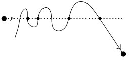 Figure 1
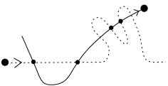 Figure 2
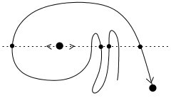 Figure 3
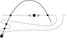 Figure 4
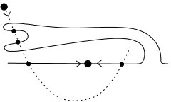 Figure 5
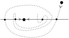 Figure 6
 Figure 7
Peer Reviews
No public reviews on file for this paper yet. If you reviewed it on a platform where reviews are public (OpenReview, ICLR, NeurIPS, ICML), you can paste yours below so the community can read it here.
Videos
No videos yet. Explain this paper in a talk, walkthrough, or lecture? Add one.
Computational complexity, torsion-freeness of homoclinic Floer homology, and homoclinic Morse inequalities.
Sonja Hohloch
Department of Mathematics and Computer Science
University of Antwerp
Middelheimlaan 1
B-2020 Belgium
Abstract
Floer theory was originally devised to estimate the number of 1-periodic orbits of Hamiltonian systems. In earlier works, we constructed Floer homology for homoclinic orbits on two dimensional manifolds using combinatorial techniques. In the present paper, we study theoretic aspects of computational complexity of homoclinic Floer homology. More precisely, for finding the homoclinic points and immersions that generate the homology and its boundary operator, we establish sharp upper bounds in terms of iterations of the underlying symplectomorphism. This prepares the ground for future numerical works.
Although originally aimed at numerics, the above bounds provide also purely algebraic applications, namely
torsion-freeness of primary homoclinic Floer homology, 2. 2)
Morse type inequalities for primary homoclinic orbits.
1 Introduction
This section is subdivided into four parts: First we recall some essential notions from homoclinic dynamics, then we give a brief introduction to classical Floer theory. Subsequently we explain the intuition behind homoclinic Floer homology before we summarize the main results of the present paper.
1.1 Notions in homoclinic dynamics
The orbit type we are interested in are the so-called homoclinic orbits whose definition we will recall in the following: Let be a manifold and a diffeomorphism. is an -periodic point if there is such that . For , such an is usually called a fixed point and the set of fixed points is denoted by .
A fixed point is called hyperbolic if the eigenvalues of the linearization of in have modulus different from . The stable manifold of a hyperbolic fixed point is given by and the unstable manifold is given by . The connected components of resp. are called the branches of resp. .
A diffeomorphism is called -orientation preserving w.r.t. if each branch of the stable and unstable manifolds of is mapped to itself.
The intersection points of the stable and unstable manifold of are called homoclinic points of and we denote the set of homoclinic points of by . An example is sketched in Figure 1.
An orbit associated to a point is the set . If is a periodic resp. homoclinic point, we call the orbit periodic resp. homoclinic. Obviously, the stable and unstable manifolds are invariant under the action
[TABLE]
Homoclinic points are somehow the ‘next more complicated’ orbit type after fixed points and periodic points. The existence of (transverse) homoclinic points was discovered by Poincaré [Poi1], [Poi2] around 1890 when he worked on the -body problem. In 1935, Birkhoff [Bi] noticed the existence of high-periodic points near homoclinic ones, but it took until Smale’s horseshoe formalism in the 1960s to obtain a formal and precise description of the implied dynamics. Since then, homoclinic points have been studied by various means like perturbation theory, calculus of variations and numerical approximation, but many questions are still open.
1.2 Classical Floer theory
In order to introduce Floer theory we need some preparations. A smooth 2n-dimensional manifold is symplectic if it admits a closed nondegenerate 2-form . For example, surfaces equipped with their volume forms are symplectic. The class of transformations associated with symplectic geometry are those diffeomorphisms that leave the symplectic form invariant, namely the group of symplectomorphisms . There is a subgroup that is particularly important for Floer theory, namely the group of Hamiltonian diffeomorphisms which is defined as follows. Given a smooth function , we set and define its (nonautonomous) Hamiltonian vector field via . Then is the associated Hamiltonian equation and its (nonautonomous) flow is called Hamiltonian flow. A Hamiltonian diffeomorphism is a symplectomorphisms which can be written as the time-1 map of a Hamiltonian flow . A Hamiltonian diffeomorphism is called nondegenerate if its graph intersects the diagonal in transversely.
Since symplectic geometry provides the framework for Hamiltonian systems it shows up naturally in physics, but, since the 1960s, symplectic geometry has also been studied for its own sake. Moser and others investigated for instance the distinction between symplectic and volume preserving geometry: in dimension two, being symplectic is the same as being volume preserving, but in dimension strictly higher than two, it differs. Symplectomorphisms are volume preserving w.r.t. the volume form , but not all volume preserving maps preserve a symplectic form.
V. I. Arnold conjectured in the 1960s that the number of fixed points of a nondegenerate Hamiltonian diffeomorphism on a closed, symplectic manifold is greater or equal to the sum over the Betti numbers of the underlying manifold. Arnold’s conjecture was open for a long time until it was proven for the -dimensional torus by Conley and Zehnder in 1983. Floer [Fl1, Fl2, Fl3] achieved a breakthrough by turning the fixed point problem into an intersection problem: he considered the fixed points of a Hamiltonian diffeomorphism as intersection points of the graph of the Hamiltonian diffeomorphism with the diagonal in the symplectic manifold . In this setting, the diagonal and the graph turn out to belong to a special class of submanifolds, the so-called Lagrangian submanifolds (submanifolds on which the symplectic form vanishes and whose dimensions are half the dimension of ); and most important, Lagrangian submanifolds have good properties concerning (Fredholm) analysis. Moreover, the intersection points of the graph and the diagonal can be seen as critical points of the symplectic action functional. Floer considered this functional as some kind of Morse function and went along to devise some kind of ‘infinite dimensional Morse theory’ for the symplectic action functional. This theory (and its generalizations) is nowadays known as Floer theory. The associated homology theory is referred to as Floer homology. Apart from leading to a proof of Arnold’s conjecture, Floer theory gave rise to many other applications in symplectic geometry, dynamical systems and other fields of mathematics and is vividly studied nowadays.
Roughly, the construction of Lagrangian Floer homology goes as follows. For details we refer the reader to Floer’s original works [Fl1], [Fl2], [Fl3] and Fukaya Oh Ohta Ono [FOOOa], [FOOOb].
Consider two transversely intersecting, ‘sufficiently nice’ Lagrangian submanifolds and lying in a ‘sufficiently nice’ symplectic manifold . Then, to two intersection points , we can assign a relative index . By fixing one as reference point one obtains an index . Now define the th Floer chain group (with -coefficients) as the free group generated by all intersection points of index , i.e.
[TABLE]
A complex structure that varies with its footpoint is usually called an almost complex structure. The corresponding generalisation of holomorphic maps are called pseudo-holomorphic maps. Now consider . The space of pseudo-holomorphic maps with and satisfying and is denoted by . This space carries the -action
[TABLE]
Dividing by this action yields
[TABLE]
which has in fact dimension . For , it is zero dimensional. Being compact, it has thus cardinality . Counting modulo 2 to be compatible with the -coefficients, we define the boundary operator
[TABLE]
on the generators and extend it by linearity. It satisfies turning into a chain complex. The associated homology
[TABLE]
is called Lagrangian Floer homology of and .
1.3 The motivation for homoclinic Floer theory
How does homoclinic Floer homology link homoclinic points to Floer theory? Remember that homoclinic points and Floer theory both involve intersecting submanifolds. Thus we have to check if the intersection problem of stable and unstable manifolds fits the requirements of Floer’s setting, i.e. are they Lagrangian? The answer is yes, under certain conditions: If we work with symplectomorphisms instead of just diffeomorphisms, the stable and unstable manifolds are always Lagrangian. But in Floer’s setting (and its generalizations), the Lagrangians are usually compact or at least ‘sufficiently nice’. Unfortunately the stable and unstable manifold are usually only injectively immersed and give rise to an abundance of intersection points as sketched in Figure 1.
Classical Floer theory knows certain techniques to deal with ‘nice non-compactness’, but they fail for stable and unstable manifolds — there are just ‘too many’ intersection points. Nevertheless, we will see in Section 2 how one can define a Floer theory for homoclinic points.
Up to our knowledge, there are few works apart from our papers [Ho1, Ho2] where homoclinic orbits are studied with symplectic methods or means related to Floer theory: Hofer Wysocki [HW] use pseudo-holomorphic curves and Fredholm theory. Cieliebak Séré [CiS] combine variational techniques and pseudo-holomorphic curves. And Lisi [Li] generalizes Coti Zelati Ekeland Séré [CZES] using Lagrangian embedding techniques.
1.4 Main results
Below in Section 2, we will describe in detail the construction of homoclinic Floer homology. Briefly, in order to compute homoclinic Floer homology, we have to locate the generators of the homoclinic chain groups and then compute the boundary operator. The generators are the so-called primary homoclinic points which are defined in (1). The computation of the boundary operator involves finding and counting certain immersions joining two primary homoclinic points. To be more precise, consider a -orientation preserving with hyperbolic. The generators, i.e. the primary homoclinic points, are intersection points of the associated (un)stable manifolds. Since the (un)stable manifolds are invariant under the -action induced by , the orbit of a generator ‘runs along the whole length’ of the (un)stable manifolds. But these are noncompact and only injectively immersed, not embedded. Therefore, a priori, we do not have any control over the whereabouts of the generators and thus in particular not over immersions joining two of them. Without upper bounds on the ‘distance’ between generators joint by immersions, finding these generators and immersions is hopeless.
The central theorem of this paper improves and maximally strengthens a result from an earlier work (to be precise, Proposition 26 and Lemma 27 in [Ho1]): In Hohloch [Ho1], we proved the existence of an upper bound, but could not give any estimates for it. The present paper gives a sharp upper bound in terms of iterations of and, in addition, also pins down certain signs associateed to the immersions. That way, homoclinic Floer homology becomes accessible and managable for numerics.
Theorem A**.**
Let be -orientation preserving with hyperbolic and use the convention . Let be the startpoint and be the endpoint of an immersion used in the boundary operator of primary homoclinic Floer homology. Then:
The endpoint lies between and on the stable and/or unstable manifold. 2. 2)
If there exists in addition an immersion with start point and endpoint for some then either or . In both cases, the immersions carry opposite signs w.r.t. the original one.
The above theorem paraphrases the content of Theorem 8 and Corollary 9. The bound in Theorem A is surprisingly low: the endpoint of an immersion is maximally just plus/minus one ‘iteration interval’ away from its start point. Together with the fact that also each primary homoclinic orbit hits an ‘iteration interval’ exactly once (cf. Lemma 2) this considerably reduces the parts of the (un)stable manifolds that have to be searched. The proof of Theorem A is not difficult, but quite tedious since one has to check a large number of (sub)cases.
Although Theorem A was originally aimed at numerical computations of homoclinic Floer homology, it has nevertheless interesting algebraic applications.
Theorem B**.**
Primary homoclinic Floer homology of -orientation preserving symplectomorphisms over is torsion-free.
This will be proven in Theorem 10. The universal coefficient theorem in homological algebra describes by means of torsion the dependence of homology groups on the chosen coefficient ring. Thus torsion-freeness implies that, for instance, homoclinic Floer homology computed with -coefficients is the same as with - or -coefficients.
Since every finitely generated abelian group has a direct sum decomposition in a finitely generated free subgroup and a unique torsion group, therefore torsion-freeness simplifies inequalities and estimates involving the rank of homology groups. The most prominent examples for such inequalities are the Morse inequalities induced by Morse homology (recalled in Section 4.1). Homoclinic Floer homology also gives rise to such inequalities:
Theorem C**.**
There are Morse type inequalities for primary homoclinic points.
This summarizes Theorem 12. Geometrically these inequalities relate and estimate the number of primary homoclinic points with different Maslov indices.
Acknowledgements
The author wishes to thank Wim Vanroose for insights into numerics.
2 Primary homoclinic Floer homology
There exist four types of Floer theory generated by homoclinic points as shown in Hohloch [Ho1, Ho2]. Each of them has different flavours and properties, but for the present paper only the following one is relevant.
Let be a symplectic manifold and a symplectomorphisms with hyperbolic fixed point and transversely intersecting (un)stable manifolds and . As already mentioned above, and are ‘highly noncompact’ (cf. Figure 1) which poses a problem for the analysis part of classical Floer theory. Fortunately there is a way to avoid this obstacle. If we restrict our studies to two-dimensional manifolds we may replace the involved analysis by combinatorics as proved by several authors (cf. de Silva [dS], Felshtyn [Fe], Gautschi Robbin Salamon [GaRS]). Restricting to dimension two simplifies only the trouble with the analysis – the difficulties related to the abundance of intersection points remain unchanged.
Now assume to be or a closed surface of genus with their resp. volume forms. This implies in particular that the (un)stable manifolds are one dimensional. Consider the set of homoclinic points where we assume the intersection to be transverse. Let , and denote by the (one dimensional!) segment between and in for . The symplectomorphism introduces a -action , on the set of homoclinic points. For transversely intersecting , the sets and are both infinite as a glance at Figure 1 shows. Denote by a continuous curve with which runs through to and through back to . We define the homotopy class of via . Then is the set of contractible homoclinic points. It is invariant under the action of .
Hohloch [Ho1] showed that there is a (relative) Maslov index for , (for ). If we assume the intersections to be perpendicular and if we flip at and at we can identify in our two dimensional setting with twice the winding number of the unit tangent vector of a loop starting in , running through to and through back to . We have for . The (relative) Maslov index yields a grading via such that for contractible homoclinic points and holds
[TABLE]
and are somehow ‘too large’ sets in order to be used as generators for a Floer chain complex. But we will find now finite subsets which can serve as generator sets for a Floer theory. is called primary if
[TABLE]
The set of primary points is denoted by . These homoclinic points have the following important properties.
Lemma 2** (Hohloch [Ho1], Remark 16, Lemma 17, and Remark 18).**
- (i)
* is invariant under .* 2. (ii)
Let be primary. Then all primary points lying in the intersection set of the same pair of intersecting branches as have a unique representative in . 3. (iii)
For a primary point holds , i.e. the Maslov index is bounded. 4. (iv)
If and intersect transversely then is finite.
We denote the equivalence class of in by . The homotopy class and the Maslov index pass to the quotient via , and .
Now we sketch the construction of Floer homology for the finite set . Consider a fixed 2-gon in with convex vertices at and . Denote its lower edge by and its upper edge by . For , with , we define to be the space of smooth, immersed 2-gons which are orientation preserving and satisfy , , and . Denote by the group of orientation preserving diffeomorphisms of which preserve the vertices and set .
Endow each branch of the (un)stable manifolds with its ‘iteration-jump direction’ as orientation and denote it by branch. When working with distinct primary points and which lie in the same branch, denote said branch by . For distinct primary points , with and associate to the orientation induced by the parametrization direction from to called . We set
[TABLE]
which was proven to be welldefined in Section 3.2 of Hohloch [Ho1]. For , set . We define the Floer chain groups and the Floer boundary operator via
[TABLE]
on a generator and extend by linearity. All groups have finite rank and, due to Lemma 2, for .
Theorem 3** (Hohloch [Ho1], Theorem 23).**
* ***
- (i)
, i.e. is a chain complex and
[TABLE]
is called primary homoclinic Floer homology of in . 2. (ii)
We have for .
The proofs of the welldefinedness of and of involve the so-called breaking and gluing procedure which mainly relies on the classification of and of immersions of relative Maslov index 2. Certain parts of the proofs are of combinatorial nature whereas other parts make use of the iteration behaviour of and use classical dynamical results like Palis’ -Lemma [Pa].
Since is finite and since also the sum in the definition of is in fact finite, we conclude:
Remark 4**.**
Primary Floer homology is completely determined by a finite number of primary homoclinic points located in (possibly large) compact segments of the (un)stable manifolds centered around the fixed point.
One aim of this paper is to determine the size of these compact segments.
3 Computational complexity
3.1 Generators and boundary operator
For the computational complexity of primary homoclinic Floer homology, we have two main steps to analyse:
- (i)
Finding of the generators, i.e. the primary points. 2. (ii)
Computation of the boundary operator, i.e. finding the connecting immersions.
There are two different aspects to pursue:
- (a)
Theoretical knowledge: Existence and welldefinedness of generators and immersions (proved in the previous work [Ho1]); enhancement and exact upper bounds of the ‘finding algorithm’ for these generators and immersions (will be done in this section). 2. (b)
Numerical realization: Actual computation of some examples by numerical methods. We aim at employing Wim Vanroose’s numerical methods based on Newton-Krylov solvers (cf. for instance Schlömer Avitabile Vanroose [SAV]). This is an ongoing project with Wim Vanroose and will be the content of a future work.
For symplectomorphisms on with compact support, Pixton’s work [Pi, Theorem C] assures the generic existence of homoclinic points for hyperbolic fixed points. On surfaces with genus, Oliveira [Ol1], [Ol2] proved generic existence under certain natural conditions. Thus we are not talking about the empty set in the following statement.
Lemma 5**.**
The first intersection point found by
- i)
starting at the hyperbolic fixed point and 2. ii)
tracing simultaneously a branch of and a branch of
is a primary homoclinic point.
Proof.
Denote by the first intersection point found by starting at the hyperbolic fixed point and tracing simultaneously a branch of and a branch of . Then by definition which implies primary. ∎
In particular symplectomorphisms that are time-1 maps coming from a perturbation of an automomous system with a homoclinic orbit do have homoclinic points (see for instance the Melnikov method, cf. Guckenheimer Holmes [GH, Chapter 4]).
Before we have a look at the positioning of generators within the branches note that symplectic diffeomorphisms are either -orientation preserving or swap the stable branches as well as the unstable branches. If is a symplectomorphism then is always -orientation preserving.
Remark 6** (Hohloch [Ho1], Remark 16 and Remark 18).**
Let be a symplectomorphism with hyperbolic fixed point and . Let be -orientation preserving and let be the branch of containing ; analogously define . Then is a representative system of all equivalence classes with .
Now let us analyse the boundary operator. Its welldefinedness is based on the following result.
Proposition 7** (Hohloch [Ho1], Proposition 26 and Lemma 27).**
Let with hyperbolic.
Let , with and . Then the immersions in are in fact embeddings. In particular . 2. 2)
Let , . Then there is such that for with we have . In particular, if the space is welldefined, then it is empty.
In order to get an upper bound on the search depth of our future algorithm we have to determine the integer in the second item of Proposition 7. Therefore we need some additional notation: Assume to be -orientation preserving. On each branch of an (un)stable manifold, we introduce an ordering via the ‘jump direction’ as follows:
- •
Let , lie in the same branch of . We write (or ) if .
- •
Let , lie in the same branch of . We write (or ) if .
The segment stands for all points and stands for all points .
Theorem 8**.**
Let be -orientation preserving with hyperbolic. Let , , and . Then
* for .* 2. 2)
If then and . 3. 3)
If then and .
This determines the integer in Proposition 7 as . The proof of Theorem 8 is technical and lengthy:
Proof of Theorem 8.
We have to check the list of the following possibilities; there is no shorter way up to our knowledge.
- •
Four cases (denoted in the following by capital Roman numbers) check where the fixed point lies w.r.t. and .
- •
Two subcases (denoted in the following by Arabic numbers) distinguish wether or not and or not.
- •
Four subsubcases (denoted in the following by small Latin characters) check if, for some , the iterate can lie in and/or or not.
Certain cases are somewhat symmetric, but since we also want to determine signs we opted for writing up the proof in full detail to avoid any confusion or even potential mistakes. Now let us begin with the proof.
(I) Case and : This implies and, by Proposition 7, .
(II) Case and :
(II.1) Subcase and :
(II.1.a) Subsubcase and : This implies implying according to Proposition 7 .
(II.1.b) Subsubcase and : This implies meaning . Moreover implying not primary .
(II.1.c) Subsubcase and : This implies implying and such that is not primary .
(II.1.d) Subsubcase and : If then and and in particular implying by Proposition 7.
If , the space may be nonempty, cf. the positioning of in Figure 2 and the absence of additional ‘interfering’ intersection points (otherwise may not be primary). Moreover, if , we observe .
If , then we get from the precendent case that and also . Thus holds, for , in particular such that .
(II.2) Subcase and : This implies immediately such that is not primary .
(II.3) Subcase and : We find such that is not primary .
(II.4) Subcase and : This is quite analogous to (II.1), but nevertheless:
(II.4.a) Subsubcase and : This implies such that by Proposition 7 .
(II.4.b) Subsubcase and : Thus and such that hindering from being primary .
(II.4.c) Subsubcase and : Thus and such that implying not primary .
(II.4.d) Subsubcase and : For , we may have cf. the positioning of in Figure 3 and the absence of additional ‘interfering’ intersection points (otherwise may not be primary). In that case, . For , we find such that . If then and .
(III) Case and : Since is -orientation preserving, lies always in the same branch as . Keep this in mind in the following.
(III.1) Subcase :
(III.1.a) Subsubcase and : Then and .
(III.1.b) Subsubcase and : Since by assumption we conclude and note which prevents from being primary .
(III.1.c) Subsubcase and : We note concluding and . For we may have cf. the positioning of in Figure 4 and the absence of additional ‘interfering’ intersection points (otherwise may not be primary). Moreover, we find in this case . If then preventing from being primary .
(III.1.d) Subsubcase and : Since we conclude . Thus and we note implying .
(III.2) Subcase :
(III.2.a) Subsubcase and : Then , thus .
(III.2.b) Subsubcase and : We conclude and . Thus there is with implying such that .
(III.2.c) Subsubcase and : We deduce and, since , we have . Thus there is with . Moreover thus .
(III.2.d) Subsubcase and : If then and . For we may have , cf. the positioning of in Figure 5 and the absence of additional ‘interfering’ intersection points (otherwise may not be primary). In that case, we observe . If then . Moreover such that . If then and . There exists with . Moreover thus .
(IV) Case and : This is quite analogous to (III), but nevertheless:
Since is -orientation preserving, lies always in the same branch as . Keep this in mind in the following.
(IV.1) Subcase :
(IV.1.a) Subsubcase and : Then and .
(IV.1.b) Subsubcase and : We conclude and . There is such that . Moreover implying .
(IV.1.c) Subsubcase and : We conclude and . There is with . Moreover implying .
(IV.1.d) Subsubcase and : We conclude and note and . For , we may have cf. the positioning of in Figure 6 and the absence of additional ‘interfering’ intersection points (otherwise may not be primary). We observe . If then implying .
(IV.2) Subcase :
(IV.2.a) Subsubcase and : Then and .
(IV.2.b) Subsubcase and : We conclude and . If we may have cf. the positioning of in Figure 7 and the absence of additional ‘interfering’ intersection points (otherwise may not be primary). In that case, as sketched in Figure 7. For , there is such that . Moreover implying .
(IV.2.c) Subsubcase and : We deduce , but then .
(IV.2.d) Subsubcase and : If then and also implying . If then . ∎
The proof of Theorem 8 implies in particular:
Corollary 9**.**
Let be -orientation preserving with hyperbolic. Let , , and . Then
If and then . 2. 2)
If and then . 3. 3)
If and then . 4. 4)
If and then , i.e. this case does not occur.
3.2 The improved algorithm
The calculation of primary homoclinic Floer homology can be optimized as summarized in the following algorithm. The results from the previous section enter in Step 5) when the necessary data for the boundary operator are determined.
Check all four pairs of branches of the stable and unstable manifolds for the existence of one intersection point using the method in Lemma 5. If one intersection point is found it is primary according to Lemma 5. 2. 2)
For all primary points , where , found in Step 1), determine all intersection points in . For transversely intersecting stable and unstable manifolds, this is a finite number . 3. 3)
For all and all intersection points of found in Step 2), determine the primary ones and remember them. According to Lemma 2, we find that way exactly one representative of each equivalence class of primary points. 4. 4)
For all and all primary intersection points in found according to Step 3), determine their Maslov index . This enables us to define the chain groups of the complex. 5. 5)
For all and all primary points in and all primary points in and with , determine
- (i)
if , 2. (ii)
and, if yes, calculate the sign .
This relies on Theorem 8 and provides all necessary information in order to calculate the boundary operator in the next step. 6. 6)
Using the already gathered information, we can now calculate
[TABLE] 7. 7)
Calculate and and .
The implementation and evaluation of this algorithm with numerical methods is an ongoing project with Wim Vanroose.
4 Torsion freeness and Morse inequalities
Apart from speeding up the calculation of primary homoclinic Floer homology, Theorem 8 has also purely algebraic applications: as we will see in this section, it implies that primary homoclinic Floer homology is torsion-free and, eventually, there are Morse type inequalities for homoclinic points.
4.1 Classical Morse inequalities
In this paragraph, we briefly sketch the approach to Morse homology via the Morse-Smale-Witten complex (cf. for instance Schwarz [Sch]).
Let be a closed -dimensional manifold. is a Morse function if, for all critical points , the Hessian of is nondegenerate. The Morse index of is the number of negative eigenvalues of . The th integral Morse chain group is defined by
[TABLE]
i.e. it is the free abelian group generated by all critical points of index . We abbreviate
[TABLE]
For a Morse function and a Riemannian metric on , the negative gradient flow is the flow of the equation
[TABLE]
Such a pair is called Morse-Smale if the intersection of stable and unstable manifolds of critical points is always transverse. Under these conditions, the space of trajectories ‘joining’ to given by
[TABLE]
has dimension . It carries the action
[TABLE]
Dividing by this action yields which has dimension . For critical points and with , the space has dimension zero and has cardinality . The trajectory spaces can actually be coherently endowed with an orientation which induces a signed cardinality
[TABLE]
This allows to define the boundary operator
[TABLE]
on the generators; it extends by linearity. It holds such that is a chain complex whose induced homology
[TABLE]
is called Morse homology. It is in fact independent of and and isomorphic to the singular homology of .
Every finitely generated abelian group has a direct sum decomposition where is a finitely generated free subgroup and is a unique torsion subgroup (that are all elements of finite order in the group ). The rank of is denoted by and is defined as the rank of . The torsion rank of is the minimal number of cyclic subgroups of whose direct sum is a subgroup.
is by definition a finitely generated free abelian group and and are as its subgroups also finitely generated and free abelian. The Morse homology groups are as quotient groups certainly abelian, but not necessarily freely generated, i.e. they may have a torsion subgroup.
Standard examples for torsion in homology groups are the higher dimensional real projective spaces. If we work with - or -coefficients, there is never torsion due to the universal coefficient theorem of homology.
If we denote by the rank and by the torsion rank of , then we certainly have for . A closer look leads to the so-called Morse inequalities (cf. also Postnikov Rudyak [PR]):
[TABLE]
where is the Euler characteristic of .
4.2 Torsion freeness and Morse inequalities for homoclinic Floer homology
We now will show that primary homoclinic Floer homology is torsion-free and we will present Morse type inequalities for primary homoclinic points using the framework of primary homoclinic Floer homology.
Theorem 10** **(Torsion freeness).
Let be a -orientation preserving symplectomorphism on or on a closed surface of genus greater than zero. Then the primary homoclinic Floer groups are free, i.e. their torsion subgroups are trivial.
The universal coefficient theorem in homological algebra describes by means of torsion the dependence of homology groups on the chosen coefficient ring. Thus torsion-freeness implies that, for instance, homoclinic Floer homology computed with -coefficients is the same as with - or -coefficients.
Before we start with the proof of Theorem 10 we recall the following fact about quotients of free groups.
Lemma 11** (Baumslag Chandler [BC], Corollary 6.17).**
Let be a free abelian group with basis and let be the free abelian group generated by where . Then is a direct sum of cyclic groups of order where if and otherwise.
We are now able to prove Theorem 10.
Proof of Theorem 10.
It is enough to consider symplectomorphisms on since, in the case of a closed surface of genus greater than zero, we may work on the universal cover as in Hohloch [Ho1].
Step 1: Let and be primary homoclinic points of relative index one. As shown in Hohloch [Ho1] in the text between Definition 9 and Definition 10, the space is either empty or contains exactly one element. According to Theorem 8, there are either exactly zero, exactly one or exactly two exponents such that is nonempty and, in the last case, the signs have opposite sign. Thus we find
[TABLE]
for all primary and with . This means that the coefficients of in the sum
[TABLE]
have never values different from . In particular, there is no common divisor of all the different from .
Step 2:
[TABLE]
is a finitely generated abelian group such that its subgroups
[TABLE]
are also finitely generated and free with
[TABLE]
In Step 1 we saw that the generators of are of the form
[TABLE]
with . Among these generators we choose a basis of . These vectors are never a multiple with absolute value of the multiplier greater than one of a basis vector of . According to Lemma 11, the quotient has no nontrivial cyclic subgroups of finite order, i.e. no torsion. ∎
Recall that, by Lemma 2, the Maslov index of a primary point satisfies . Therefore only primary homoclinic Floer chain groups with can be nontrivial such that the complex looks like
[TABLE]
We have
[TABLE]
and we set . Due to Theorem 10, the torsion rank of vanishes and we find
Theorem 12** **(Homoclinic Morse inequalities).
For the rank of the primary homoclinic Floer chain and homology groups holds:
** 2. 2)
** 3. 3)
** 4. 4)
**
Proof.
Due to Theorem 10, the torsion rank vanishes. We estimate
. 2. 2)
For and holds:
[TABLE] 3. 3)
follows from 1) and 2). 4. 4)
Let with . W.l.o.g. we assume . Keep in mind that thus . First consider the case even. Then we have
[TABLE]
The case odd follows similarly which finishes the proof.
∎
The reference list from the paper itself. Each links out to its DOI / PubMed record.
- 1[BC] Baumslag, B.; Chandler, B.: Theory and problems of group theory , Schaum’s outline series, Mc Graw-Hill 1968.
- 2[Bi] Birkhoff, G. D.: Nouvelles recherches sur les systèmes dynamiques , Mem. Pont. Acad. Sci. Nov. Lyncaei, 1935, 53 , 85 – 216.
- 3[Ci S] Cieliebak, K.; Séré, E.: Pseudo-holomorphic curves and multiplicity of homoclinic orbits , Duke Math. J. 77 No. 2 (1995), 483 – 518.
- 4[CZES] Coti Zelati, V.; Ekeland, I.; Séré, E.: A variational approach to homoclinic orbits in Hamiltonian systems , Math. Ann. 288 , 133 – 160 (1990).
- 5[d S] de Silva, S.: Products in the symplectic Floer homology of Lagrangian intersections , Thesis, Merton College, Oxford 1998.
- 6[Fe] Fel’shtyn, A.: Dynamical Zeta functions and Floer homology , Contemporary Mathematics, Vol. 385 (2005), 187 – 203.
- 7[Fl 1] Floer, A.: A relative Morse index for the symplectic action , Comm. Pure Appl. Math., Vol. 41 (1988), 393 – 407.
- 8[Fl 2] Floer, A.: The unregularized gradient flow of the symplectic action , Comm. Pure Appl. Math., Vol. 41 (1988), 775 – 813.