TL;DR
This paper presents a neural network-based system for estimating the volume of the left ventricle from MRI images, combining segmentation and volume estimation techniques, and achieving competitive results in a Kaggle competition.
Contribution
It introduces an end-to-end deep learning approach with a novel training strategy using multiple datasets and a variance estimation method for improved LV volume prediction.
Findings
Ranked 4th in the Kaggle competition
Effective integration of segmentation results for volume estimation
Demonstrated the utility of multi-dataset training with different labels
Abstract
Segmenting human left ventricle (LV) in magnetic resonance imaging (MRI) images and calculating its volume are important for diagnosing cardiac diseases. In 2016, Kaggle organized a competition to estimate the volume of LV from MRI images. The dataset consisted of a large number of cases, but only provided systole and diastole volumes as labels. We designed a system based on neural networks to solve this problem. It began with a detector combined with a neural network classifier for detecting regions of interest (ROIs) containing LV chambers. Then a deep neural network named hypercolumns fully convolutional network was used to segment LV in ROIs. The 2D segmentation results were integrated across different images to estimate the volume. With ground-truth volume labels, this model was trained end-to-end. To improve the result, an additional dataset with only segmentation label was used.…
Click any figure to enlarge with its caption.
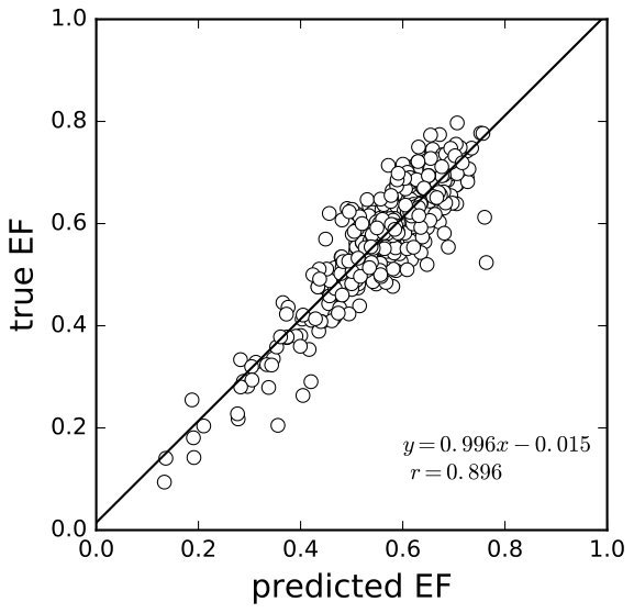 Figure 1
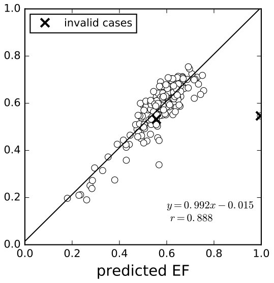 Figure 2
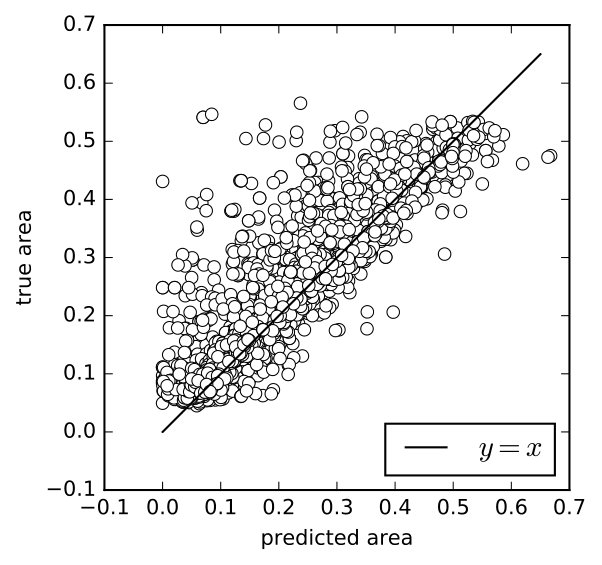 Figure 3
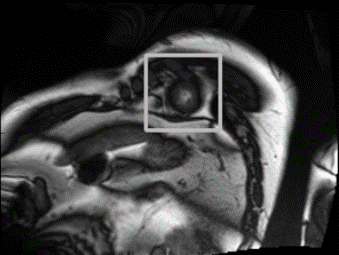 Figure 4
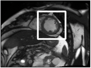 Figure 5
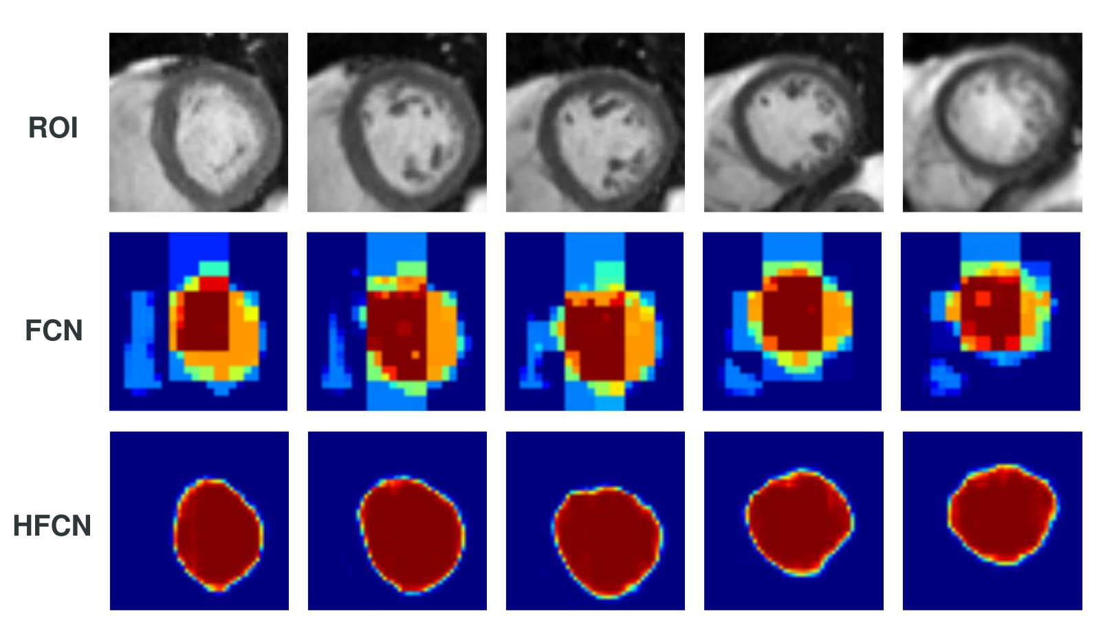 Figure 6
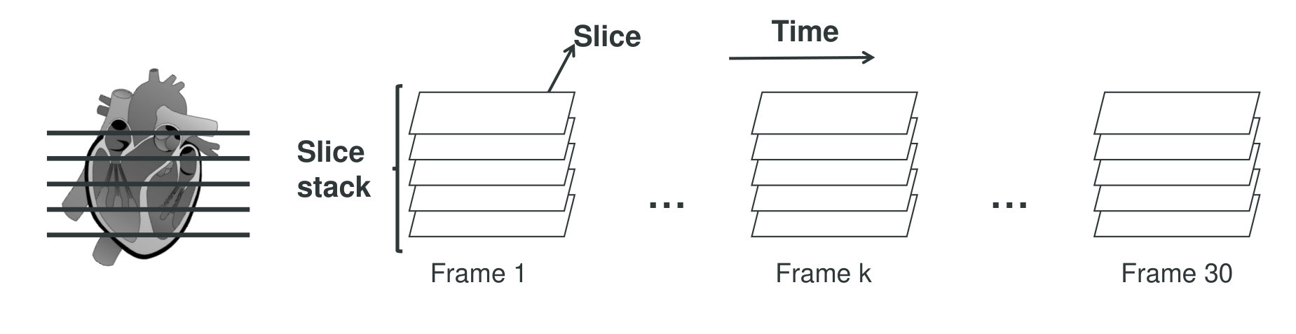 Figure 7
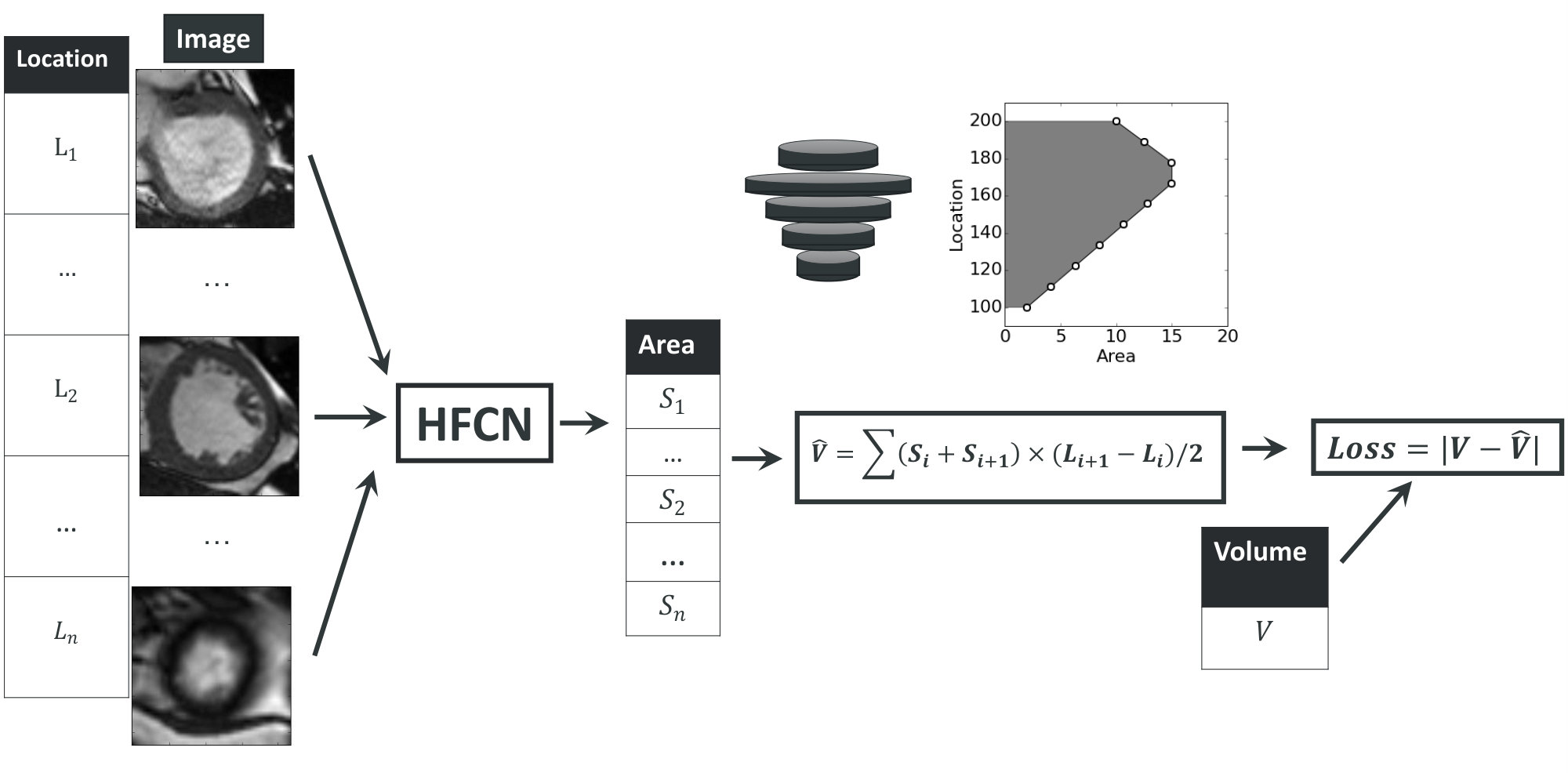 Figure 8
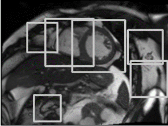 Figure 9
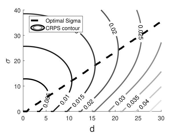 Figure 10
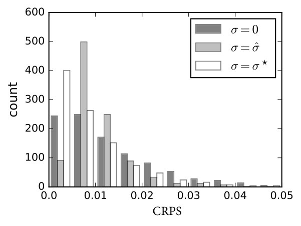 Figure 11
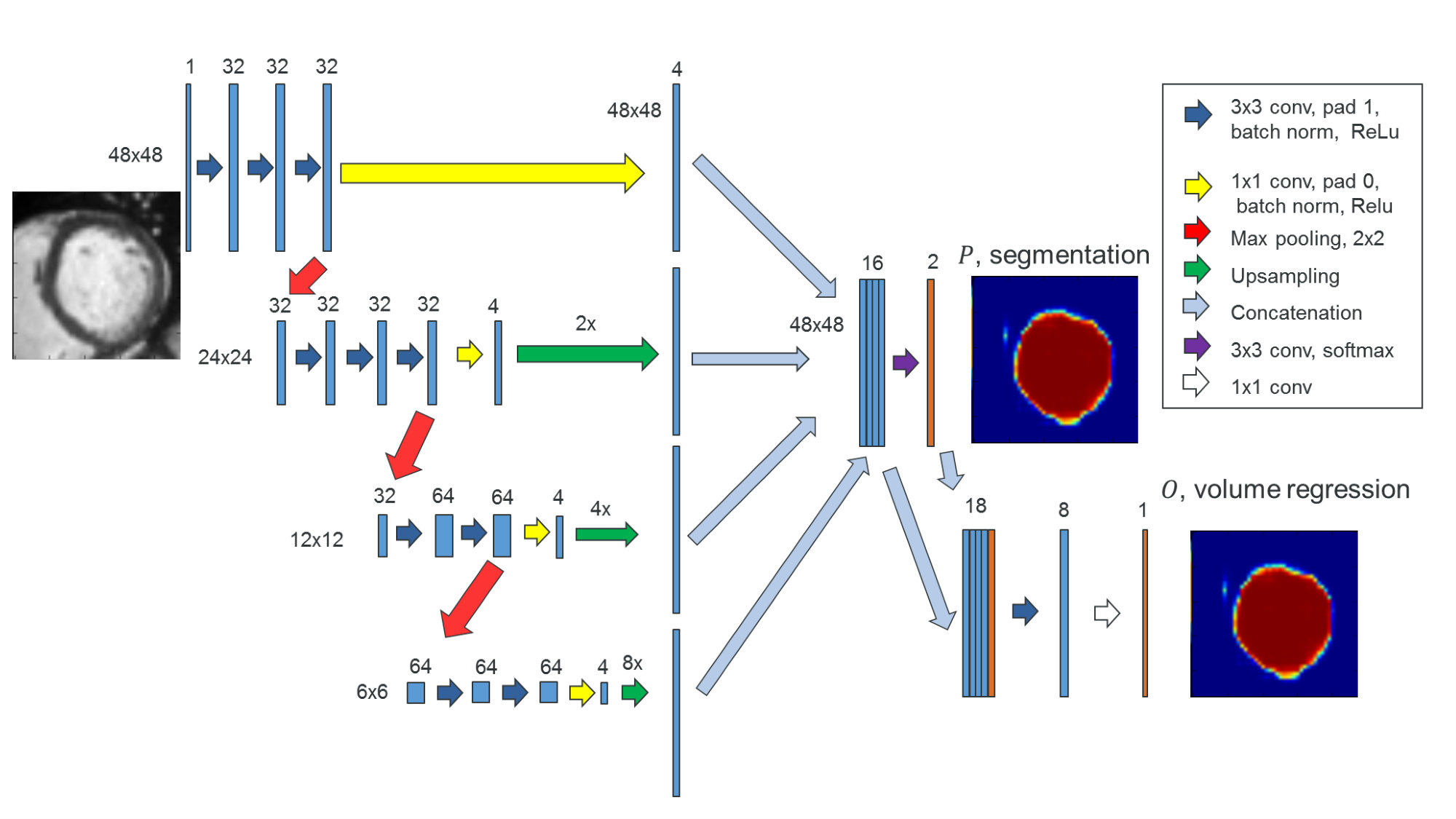 Figure 12
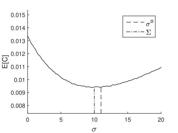 Figure 13
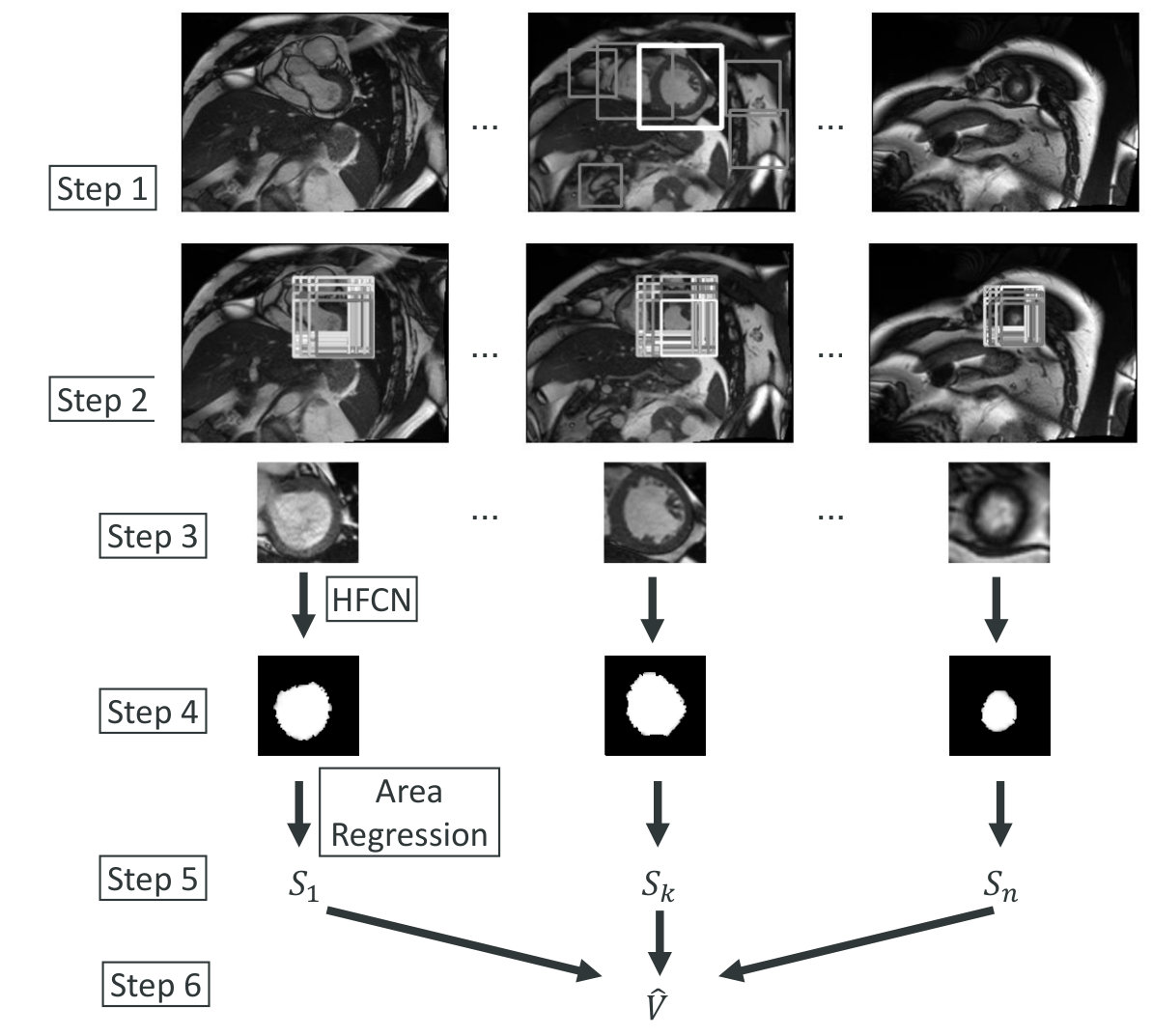 Figure 14
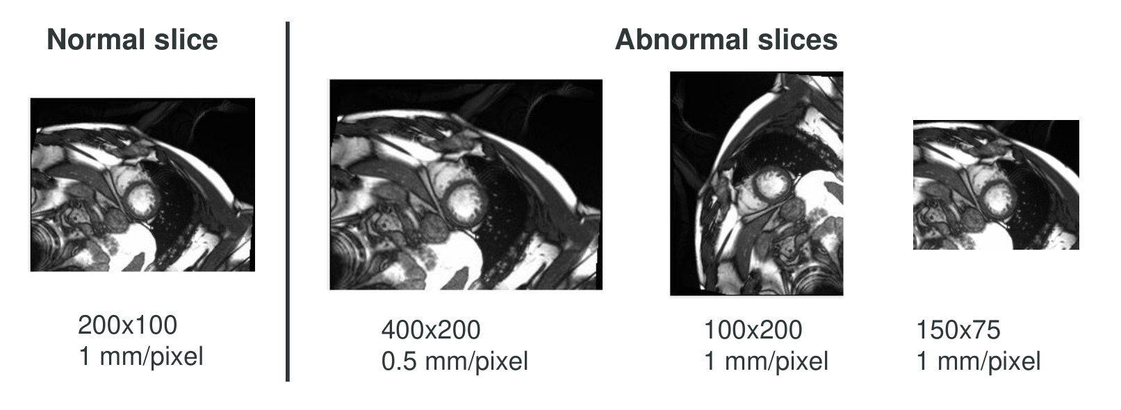 Figure 15
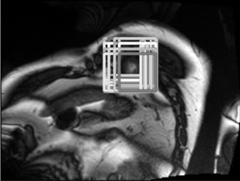 Figure 16
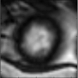 Figure 17
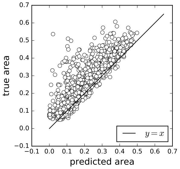 Figure 18
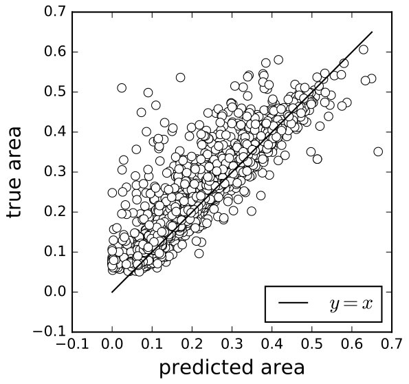 Figure 19
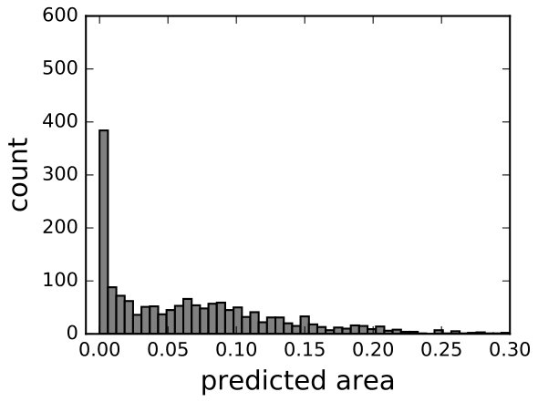 Figure 20
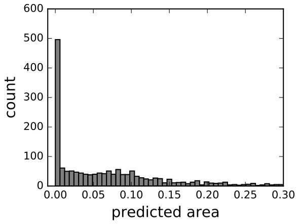 Figure 21
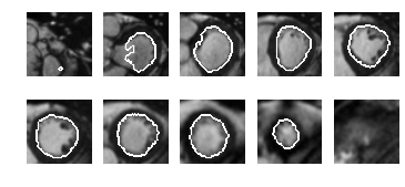 Figure 22
 Figure 23
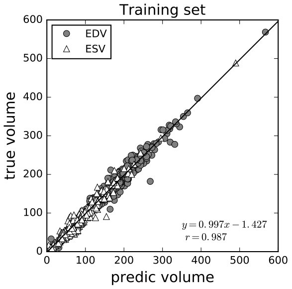 Figure 24
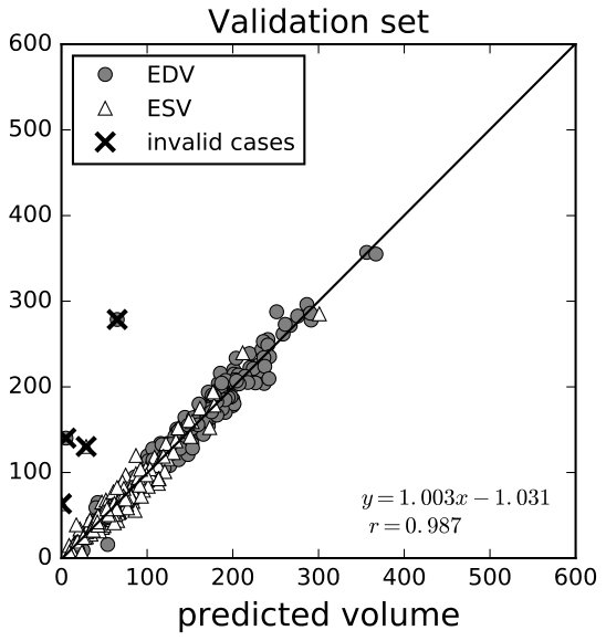 Figure 25
| Layer | Data | Conv1 | Pool1 | Conv2 | Pool2 | Conv3 | Pool3 | Classifier | ||||||||||||||
|---|---|---|---|---|---|---|---|---|---|---|---|---|---|---|---|---|---|---|---|---|---|---|
| Param |
|
|
|
|
|
|
Ave, 6x6 | Softmax | ||||||||||||||
| Size | 25x25x6 | 25x25x32 | 12x12x32 | 12x12x32 | 6x6x32 | 6x6x32 | 1x1x32 | 1x1x2 | ||||||||||||||
| St: stride, BN: batch normalization, Drop: dropout ratio, Ave/Max: average/max pooling | ||||||||||||||||||||||
| Training | Validation | Test22footnotemark: 2 | |
|---|---|---|---|
| 0.01358 | 0.01550 | 0.01400 | |
| 0.00999 | 0.01280 | 0.01067 | |
| 0.00949 | 0.01112 | - |
Peer Reviews
No public reviews on file for this paper yet. If you reviewed it on a platform where reviews are public (OpenReview, ICLR, NeurIPS, ICML), you can paste yours below so the community can read it here.
Code & Models
Videos
No videos yet. Explain this paper in a talk, walkthrough, or lecture? Add one.
Estimating the volume of the left ventricle from MRI images using deep neural networks
Fangzhou Liao, Xi Chen, Xiaolin Hu, and Sen Song Fangzhou Liao and Sen Song are with the School of Medicine, Tsinghua University, Beijing 100084, China.Xi Chen and Xiaolin Hu are with the State Key Laboratory of Intelligent Technology and Systems, Tsinghua National Laboratory for Information Science and Technology (TNList), and Department of Computer Science and Technology, Tsinghua University, Beijing 100084, China. (email: [email protected]). This work was supported in part by the National Basic Research Program (973 Program) of China under Grant 2013CB329403, and in part by the National Natural Science Foundation of China under Grant 61273023, Grant 91420201, and Grant 61332007.
Abstract
Segmenting human left ventricle (LV) in magnetic resonance imaging (MRI) images and calculating its volume are important for diagnosing cardiac diseases. In 2016, Kaggle organized a competition to estimate the volume of LV from MRI images. The dataset consisted of a large number of cases, but only provided systole and diastole volumes as labels. We designed a system based on neural networks to solve this problem. It began with a detector combined with a neural network classifier for detecting regions of interest (ROIs) containing LV chambers. Then a deep neural network named hypercolumns fully convolutional network was used to segment LV in ROIs. The 2D segmentation results were integrated across different images to estimate the volume. With ground-truth volume labels, this model was trained end-to-end. To improve the result, an additional dataset with only segmentation label was used. The model was trained alternately on these two datasets with different types of teaching signals. We also proposed a variance estimation method for the final prediction. Our algorithm ranked the 4th on the test set in this competition.
Index Terms:
Medical Image Analysis, Deep learning, Image segmentation, Regression
I Introduction
In cardiovascular physiology, the volume of the left ventricle (LV) is important in heart disease diagnosis. The difference of end diastole volume (EDV) and end systole volume (ESV), that is EDV-ESV, reflects the amount of blood pumped in one heart beat cycle (Stroke Volume, SV), which is often used in the diagnosis of heart diseases. Another frequently used indicator is the ratio (EDV-ESV)/EDV (Ejection Fraction, EF).
Modern medical imaging methods such as ultrasound, radiology and MRI make it possible to estimate the volume of LV. The first step is to acquire a set of slices along the -axis (the long axis of the LV). Then experienced doctors draw contours on the slices to get the area of LV in each slice and calculate volume by accumulating the areas along the -axis. This step is time-consuming. Usually, an MRI stack costs a senior doctor more than ten minutes in the analysis. If an automatic method is available, it will speed up the diagnosis process.
A straightforward approach for solving this problem is to first segment LV area in each MRI slice, then estimate the volume of LV by integrating the areas across difference slices. Over years many LV segmentation algorithms have been proposed (e.g., [1, 2, 3]). But the progress towards solving the problem was hindered by the lack of benchmark dataset. The first large public available dataset called the Sunnybrook dataset was released in 2009 [4], which contains hundreds of cases. It provides not only the diagnosis label for each case but also LV contours labeled by experts for some cases. It is the first systematically labeled dataset, which facilitates the application of machine learning algorithms on this problem, including deep neural network [5, 6] and random forest [7]. Traditional learning-free methods can also benefit from it [8, 9].
In 2015 Kaggle.com organized a competition named “Second National Data Science Bowl”. A dataset with hundreds of 3D MRI videos were provided with EDV and ESV labels. The task was to predict EDV and ESV in new videos [10]. External data except the Sunnybrook dataset was not allowed to be used. Clearly, a single scalar volume label is quite uninformative for training an accurate model because the volume depends on the classification of every pixel in each slice. To make the model capable of doing segmentation, we proposed to train a deep neural network using both the volume labels on the training set and the segmentation labels on the Sunnybrook dataset. The proposed pipeline was based on deep neural networks. The competition had two rounds. In the initial round there were more than 700 teams, and in the final round there were 192 teams. Our algorithm ranked the 4th in the final round. In the paper, we describe our algorithm in detail to make a contribution to related clinical practices111The source codes are released on https://github.com/lfz/Heart-Volume-Estimation.git..
II Related work
II-A Deep learning models for general image segmentation
Before the rise of deep learning, most image processing algorithms rely on sophisticated handcrafted features (e.g. HOG [11], Haar [12], SIFT [13], LBP [14]) and complex classifiers (e.g. random forest, support vector machine, cascade classifier). Deep learning provides an end-to-end solution to these tasks because in these models both features and classifiers are learned together. Now deep learning is enjoying fast development for computer vision tasks including image classification, object detection, image segmentation and so on. See reference [15] for a recent review. As image segmentation is one of the main parts in our pipeline, we briefly review existing deep learning models for general image segmentation below.
According to whether there is upsampling operations, existing deep learning models for image segmentation can be classified into two categories. The first category of models do not use upsampling because they use patches as inputs and classify their central pixels [16, 17]. This process slides on the image to predict the label of every pixel. It is slow because every single patch requires a feedforward computation. However, recently this problem was partially solved by rarefying the weight [18, 19].
The other category of models takes an image as input and output a label map. They usually use deconvolution or unpooling to upsample the Low-resolution, high-level representation of an image back to the original size. For example, the fully convolutional network (FCN) [20] uses a pre-trained network as an encoder, then learns a decoder at different levels and combine them together to achieve finer result. In the hypercolumns network [21], features in different levels are concatenated together, and segmentation is conducted based on this new layer with multi-scale information. The U-Net [22] introduces an U-shape network architecture which is more efficient in capturing fine-scale information. The deconvolution network [23] stores indexes in the max-pooling layer in the encoding step, and uses them in corresponding unpooling layers in the decoding step. An advantage of these models is their fast prediction due to the fully convolution style.
II-B MRI image segmentation
MRI is currently an important imaging technique for cardiology and its data is widely used in segmentation algorithm development. Lorenzo-Valdés et al. [1] built a standard heart atlas and registered every slice stack to it. Kaus et al. [2] used a deformable model to build 3D model first and segmented the inner surface in 3D space. Lynch et al. [3] used a level-set method and took temporal information into consideration. Eslami et al. [24] proposed a guided random walk method. Instead of finding the LV chamber, they targeted for segmenting the ventricle wall. Nambakhsh et al. [25] proposed a convex relaxed distribution matching algorithm which finds the best segmentation that matches the intensity/shape prior distribution. Zhang et al. [26] adopted active appearance and shape models to build a general model of the heart shape.
In recent years, researchers began to apply deep learning algorithms to LV segmentation problem. Ngo et al. [27] used a deep belief network (DBN) and combined it with level-set method [28]. Avendi et al. [6] combined a multilayer perceptron with deformable model [29]. One reason for that both works incorporated traditional methods (level set method and deformable model) is that the models were trained on the Sunnybrook dataset, which is too small to train complex and powerful models. Given this, Tran [30] collected multiple datasets and trained an end-to-end model (FCN) on them.
Though the task in the “Second National Data Science Bowl” competition organized by Kaggle.com was to estimate the volume of LV, many teams (including our team) chose to segment LV in every slice of MRI images as an important step. The first place and third place teams adopted this strategy and used extra hand-labeled data to increase the number of training samples for segmentation task [31, 32], which we think is the primary reason for their better performance than our model. The second place team trained end-to-end models to directly predict the volume value without using segmentation labels. The final result was based on an ensemble of 44 models [33], yet we just used a single model. All of the top four teams built their models based on deep convolutional neural network.
III Volume estimation
III-A Data preprocessing
The training, validation, and test set consist of 500, 200, and 440 cases respectively. Each case has several views: short axis view (sax), 4-chambers view (4-ch), and 2-chambers view (2-ch). Each view is a 4D data: -axis (2D frame) -axis (slice location) -axis (imaging time). We only used the sax view data in this competition. Each slice location is usually sampled 30 times, which correspond to 30 frames, in a heart-beating cycle (1(a)). In this paper a frame may refer to a slice stack (3D) or a slice (2D) according to the context. To get better results, we used 630 cases for training and 70 cases for validation.
On the training set and validation set, two volume values of LV were provided for each case corresponding to ESV and EDV respectively, but their corresponded end of systole frame (ESF) and end of diastole frame (EDF) were not provided. We identified the two frames for each case with visual inspection which had minimum and maximum volumes, respectively. Then each case had two frames with volume labels. They were used in the volume fine-tuning part (subsubsection III-G2).
In some cases, spatial resolution, orientation, and size can be different from slice to slice (1(b)). That information is stored in metadata of each dicom file. According to these information, the inconsistent slices were rotated/resized/cropped/padded to be consistent with most slices.
We used Sunnybrook dataset as a supplementary dataset. It also consists of three sets: training, validation, and test. It has human-labeled LV contour (both inner contour and outer contour) for some cases which were used in this competition. We combined these three sets together and extracted 400 slices with outer contours of LV for the detection task (Section III-C). We also extracted 725 slices with inner contours of LV for the segmentation task (Section III-F).
III-B Overview of our method
We first show the overview of the proposed pipeline (Fig. 2), then in subsequent sections we describe the individual steps in detail.
First, we trained an LBP [34] cascade detector to produce some ROI proposals about the location of LV in the middle slice of the first frame. Since the visual appearance of LV was prominent (a concentric circle), especially in the middle slice, the correct ROI was always included in the proposals. Then a CNN was applied to classify those proposals and the one with the highest score was chosen as the ROI. See Fig. 2, Step 1.
Second, we extended the ROI to all frames and all slices, and segmented the LV in each ROI and calculated the area based on a modified FCN, called hypercolumns fully convolutional network (HFCN, [21]). This model was trained on the Sunnybrook dataset. See Fig. 2, Steps 2 to 4.
Finally, for each slice, we calculated areas based on the model in the previous step and got the volume by integrating areas along the -axis. Since the min and max volume labels for every case (ESV and EDV, respectively) were available, the error signal could be used to fine-tune HFCN. See Fig. 2, Steps 5 to 6.
III-C ROI proposal in the middle slice of the first frame
Since LV is relatively small in each slice, performing segmentation on the whole image is very challenging. It would be nice if we could have a finer ROI bounding the LV in every slice. Since LV, like a spindle, is big at the middle and small at the two ends, if we can localize the ROI in the middle slice, then this bounding box should also bound LV in other slices.
Face detection is a similar problem and has been studied for years in computer vision. We chose a very simple algorithm used in face detection: built a cascade classifier based on LBP features. We extracted 400 positive ROIs from the Sunnybrook dataset and semi-automatically labeled 500 positive ROIs in the training dataset, then trained the cascade classifier with ten times more negative samples.
Since concentric circle may appear in other locations in the body, this approach produced some false-positive ROIs. But the correct ROI was among the proposals in almost all cases. And this bounding box was usually tight enough. Another classifier was then used to choose the correct ROI. See below.
III-D ROI classification in the middle slice of the first frame
The most distinctive feature of the heart lies in the spatial-time domain: the heart is beating. Yet it can not be captured by the method described above. To utilize the information of “heart beating”, for each case, 6 frames were evenly chosen from 30 frames in the time series and concatenated together, so that the top and bottom channel images were diastole and the middle channel image was systole. Then all proposals given by the LBP detector were extended to these frames, resized to and manually labeled as correct or wrong. Then a 3-layers CNN was trained to perform classification (Table I). As a simple way of data augmentation, all positive samples were rotated by . After trained in 500 cases, the detection system obtained 100% accuracy on the validation set (3(a),3(b)).
III-E ROI localization in other slices and other frames
The previous step gives an accurate bounding box at the middle slice of the first frame. The simplest way to have ROI in all frames and slices is to copy the result from this slice. It is acceptable in the time-domain as LV does not change too much in the heart-beating cycle. But because the shape of LV is like an upright spindle, the bounding box in the middle slice is too large for other slices. So a refinement step for the bounding box of other slices in the first frame is necessary. Starting from the middle slice, we extended the ROI to other slices sequentially in bottom-up and top-down directions respectively. Each slice inherited the ROI of its neighboring slice determined in the last step as the initial guess and refined it with the method described below. Many square patches were extracted around the initial guess with different corner point whose length ranges from 0.6 to 1.1 times the length of the initial guess (similar to sliding window, 3(d)). For each patch, we chose 6 frames in time series and concatenated them as described in Section III-D, then fed them to the 3-layer CNN mentioned above (Table I), which gave us a confidence score for every patch. The patch with the highest score was the refined ROI. In some cases where the slice location was beyond the range of LV in the -axis so that LV was absent or the shape of LV is abnormal, the classifier would give a low score for every patch. Under such circumstances, we chose the ROI in its nearest slice as its own.
After the bounding boxes in all slices in the first frame were obtained, they were extended to corresponding slices in other frames directly.
III-F Segmentation
After refining ROIs, the target area usually occupied 20-50% of the ROI. All ROIs were resized to . The next step was to segment LVs and estimate their areas in individual slices.
We first tried the fully convolutional network (FCN) [20] for segmentation. It received a 2D image as input and gave a binary segmentation result. The training set was obtained from the Sunnybrook dataset. Although FCN uses multiscale information, its predictions in different levels are independent. The final result is just an average of those predictions. It is an inefficient way of integrating multiscale information. Our experiments validated this point. To overcome this shortage, we adopt the idea of hypercolumns [21]. Features from different levels were concatenated to form a new layer, and segmentation was based on this new layer (Fig. 4). This model is termed hypercolumns FCN (HFCN) in this paper.
III-G Volume estimation
III-G1 Naive volume calculation
After training HFCN, we fed the ROI in every slice to it and got an output image whose pixel value was the likelihood of being part of LV. By binarizing and averaging all pixel value, we could get the area fraction of LV in this slice. As the pixel resolution and image size was known, the physical area of LV could be deduced. The whole process is formulated as follows:
[TABLE]
where is the input ROI, is the output image whose pixel value is the probability of being part of LV, is parameters of HFCN, is area fraction, is physical length of a pixel, is patch length, and is physical area. These steps can be combined in one step:
[TABLE]
The next step was to calculate the volume based on the areas at different locations in the -axis. We assume the cross section of LV is always a circle. Then the volume between two neighboring slices is a truncated circular cone, whose volume is
[TABLE]
where is the area of LV in the -th slice and is the coordinate of the -th slice in the -axis. The total volume of LV is the sum of all truncated cones:
[TABLE]
where is the number of slices.
III-G2 Fine-tuning with volume labels
If the segmentation results were perfect, the volume given by Equation (4) was exact. Unfortunately, the segmentation network did not work perfectly partly due to the small size of the training set. To augment the dataset, every case was augmented by rotating . To further improve the results we needed to utilize the volume labels of the dataset provided in this competition to fine-tune the segmentation network.
We chose -norm loss function instead of the usually used -norm loss function:
[TABLE]
where is the ground truth volume. The reason is as follows. The labels were variant due to subjective standards of different doctors, even misleading in some cases222For instance, the sax view data of the case 429 in the training set, and cases 595 and 599 in the validation set were incomplete, though the 4-ch view data of them were complete. The labels of these cases, though might be correct as doctors could estimate the volume in the 4-ch view, were misleading to our algorithm, since it worked solely on the sax view. . It is well-known that the -norm loss is more robust to outliers than -norm loss. Another reason was that the -norm loss is more similar to the evaluation function used in the competition, which will be discussed in Section IV-A.
To this end, the estimated should be a differentiable function of the network parameters . Note that all Equations (1) to (4) meet this requirement except Equation (1b). One solution is substituting it with a sigmoid activation function: But because the output of the sigmoid function is always between 0 and 1, a consistent positive bias for non-LV pixels and negative bias for LV pixels will be caused. In our algorithm. We used another method instead.
We concatenated with its previous layer to form a new layer. Then a convolutional layer was added after it (see Fig. 4). This was essentially a linear regression. Surprisingly, we found that it worked better than the sigmoid transformation.
Denote the new output by , and the new set of parameters by :
[TABLE]
Then Equation (1c) becomes
[TABLE]
Though Equation (3) is differentiable, the presence of makes training unstable. We empirically found that substituting it with the arithmetic mean made learning more robust. In other words, Equation (3) is changed to
[TABLE]
The whole diagram for volume estimation is shown in Fig. 5.
III-H Alternate training
Though our goal was to estimate the volume of LV, simply training the model using the volume labels provided by the competition organizer did not work well. This was because the estimation quality heavily relies on the image segmentation results, but the organizer did not provide ground-truth labels for segmentation. Our solution was to alternately train the model on the competition dataset with volume labels and on the Sunnybrook dataset with image segmentation labels.
In other words, both two outputs of HFCN network (see Fig. 4) were used in training. The first one, , was used in the segmentation task, and the second one, , was used in the volume regression task. These two tasks were trained alternately. Specifically, a training block was composed of a segmentation epoch and a volume regression epoch. This scheme made the most use of limited label resources and made these two tasks regulizers of each other to reduce over-fitting. To achieve higher precision in volume regression, we removed segmentation epochs in training after 100 blocks. Then the training continued with only regression epochs until convergence. A total of 200 blocks were used in training. The learning rate was set to 0.001 with momentum of 0.9, and discounted by 0.1 every 70 blocks.
III-I Re-picking of ESF and EDF
As mentioned before, we picked the ESF and EDF in the training set by visual inspection. But it was potentially inaccurate. So after training, we fed every slice of a case in the training set to the model and identified its ESF and EDF by finding the min and max volumes from model outputs. Then we re-trained the segmentation network based on the new ESF and EDF.
IV Distribution estimation
IV-A Evaluation function
The evaluation function in this competition was Continuous Ranked Probability Score (CRPS). Participants were required to upload a distribution of predicted volume (EDV or ESV) over all possible volumes (The upper limit was set to 599 because no ground truth value was larger than this value). Say for the -th case, the ground truth value is . Then the ground truth distribution is a delta function peaked at . Clearly its cumulative distribution function (CDF) is
[TABLE]
Denote the predicted probability density function (PDF) and its CDF for the -th case by and , respectively. The CRPS for each estimation is defined as a distance between and :
[TABLE]
where can be EDV or ESV. The evaluation metric is the mean CRPS over both and all .
IV-B Generation of a distribution
Note that the proposed algorithm can only give a single value for any case but does not give a distribution over all . In the simplest case, is a delta function peaked at , then is a step function, and CRPS becomes . This is another reason why we used -norm loss for volume fine-tuning. However, we found that the delta function is not a good choice.
To better understand the properties of this evaluation function, by assuming the distribution to be the PDF of , we numerically calculated the distribution of CRPS (9(a)) on and . We found that could significantly influence performance. For example, , , which led to more than 40% reduction. We found that for every there existed an optimal that minimized CRPS, and was approximately a linear function of . But since was unknown during test, this was only used as a performance reference on the training set.
Let be the discrete PDF of . Since is known the problem reduces to find an optimal . A natural choice of is , and by numerical experiment, we found that this choice is good enough though not optimal (see Appendix). By combining Equations (1c)(4)(8), we know that can be written as a linear summation of :
[TABLE]
We assume that and are independent when , then the variance of is also a linear summation of variance of :
[TABLE]
can be estimated from data in 7(b). Specifically, we collected all dots with predicted area in the range , and calculated the variance of their true areas. Because this variance stands for the probable dispersion of true area given the predicted area, it is used as .
Finally we used a modified form where was a hyperparameter hand-tuned on the validation set. The reasons are as follows. First, the neighboring slices are similar, so and are not independent. Second, the distribution of samples used to compute (7(b), extracted and augmented from Sunnybrook dataset) might deviate from that of the competition dataset, so the computed variance was not the desired value. Based on the evaluation performance on the validation set, the best was 0.5.
V Results
V-A Image segmentation
For image segmentation, we trained the model on all data of the Sunnybrook dataset including the training set, validation set, and test set. The training accuracy was 98.3% without fine-tuning using the volume information of the Kaggle competition dataset, and this accuracy dropped to 97.2% after alternate training on both datasets.
Fig. 6 shows the segmentation results of a slice stack in the Kaggle training set. Qualitative inspection reveals that the results are satisfactory. The first and last slices exceeded the range of LV, and the model predicted very few pixels belonging to LV. The second slice contained an exit of LV, and the model correctly found this C-shape structure. For the middle slices, the papillary muscles (dark tissue in LV) were correctly segmented as belonging to LV.
V-B Area estimation
To evaluate the areas estimation performance of our model, we extracted all available patches from Sunnybrook dataset and augmented the number to 5000 by flipping, scaling, and shifting. We also manually selected 1000 negative samples, but because the authors are not professional doctors, there might be some false negative samples. Then we predicted the areas in these images according to Equations (2) and (6) respectively, and compared their predicted values to the ground truth values (ground truths value are calculated from the human-labeled contours). With Equation (2), the predicted values of positive samples were, on average, smaller than the ground truth (7(a)), and the values of some negative samples were greater than 0 (7(c)). With Equation (6), both problems were attenuated to certain extent (7(b), 7(d)).
V-C Volume estimation
Unlike the procedure in the training stage, where the frames corresponding to diastole and systole state were given, in this stage, we estimated the volumes of all frames in one case and treated the minimum and maximum of these values as ESV and EDV, respectively.
The results on the training and validation sets are shown in 8(a), 8(b). Qualitatively, the regression was good enough, except for some outliers that might be caused by incompleteness of data or incorrect labels. Quantitatively, on the validation set, the average relative error was 13.1% for ESV and 8.59% for EDV, and the correlation coefficients between the predicted volume and the ground truth volume were both 0.987. The average -norm error of EF was 3.93% (for regression result, see 8(c), 8(d)), and the correlation coefficient between the predicted EF and the ground truth was 0.888 (8(d)).
After the competition, the organizer analyzed the results of the leading teams on test set [35]. According to the report, in terms of the root mean square error (RMSE) of EF, we achieved the best result in top 4 teams. And in terms of RMSE of EDV and ESV, we also ranked 2nd and 1st, respectively (Table II). Unfortunately, the evaluation metric for this competition was not based on any single value estimation but based on the distribution estimation.
V-D Evaluation result
We tested the effect of our variance estimation method (Table III). The distribution of CRPS over the training set is plotted in 9(b). Our method was much better than and was very close to the result of . The mean CRPS on the test set was 0.010666, which ranked the 4th in the competition (Table II). Because we do not know the labels of the test samples, we can not do further analysis.
VI Discussion
We used a deep convolutional neural network (DCNN) to segment human MRI images and estimate LV volume. It exhibited good performance in a Kaggle competition. The greatest difficulty in this competition was the lack of informative labels. Our solution was volume fine-tuning and alternate training, which enabled the DCNN to receive supervising signals from both segmentation labels in the Sunnybrook dataset and volume labels in the Kaggle dataset. As far as we know, it is the first 2D segmentation network fine-tuned by utilizing 3D volume labels.
One limitation of our algorithm is that it does not make use of the prior knowledge of the 3D shape of LV, e.g. smoothness of the 3D surface. Neither does it use the smoothness of LV shape in the time domain. As a result, sometimes the model produced segmentation results with two isolated LV regions or a region with a highly irregular shape. This problem can potentially be solved by 3D CNN, or conditional random field as post-processing, which is left for future exploration.
As a powerful tool in computer vision, deep neural network draws more and more attention in biomedical image processing area. As an evidence, in this competition all of the top 4 teams based their algorithms on DCNN. In biomedical image processing, the image features are influenced by lots of parameters: age and gender of patients, viewing angle and position, instrument parameter, and even subject biases of doctors. Traditional methods entail much effort on ruling out those unwanted factors. But DCNN can learn useful features from a large dataset automatically. As long as the training set is large enough to cover all varying factors, DCNN could be robust to them. We believe that DCNN will play more and more significant roles in biomedical image processing.
Appendix A Optimal given prediction variance
If we parameterize Equation (9) as , according to the definition of :
[TABLE]
But in the test stage the exact value of is unknown. What we have is the estimated value and the estimation variance , based on which we know the distribution of . And we want to have an optimal choice of so that the expectation of Equation (9) is minimized:
[TABLE]
where is the PDF of .
Since this equation is intractable, we conducted a numerical simulation, i.e. for each , sampled 100,000 and computed their average CRPS. The result is shown in Fig. 10. It turned out that was very close to and their corresponding were also very close:
[TABLE]
In this experiment, was set to 10 and was set to 100, which were typical values in this study. We found that this conclusion was robust in a wide range of and .
The reference list from the paper itself. Each links out to its DOI / PubMed record.
- 1Lorenzo-Valdés et al. [2002] M. Lorenzo-Valdés, G. I. Sanchez-Ortiz, R. Mohiaddin, and D. Rueckert, “Atlas-Based Segmentation and Tracking of 3D Cardiac MR Images Using Non-rigid Registration,” in Proceedings of International Conference on Medical Image Computing and Computer Assisted Intervention . Springer Berlin Heidelberg, Sep. 2002, pp. 642–650.
- 2Kaus et al. [2004] M. R. Kaus, J. von Berg, J. Weese, W. Niessen, and V. Pekar, “Automated segmentation of the left ventricle in cardiac MRI,” Medical Image Analysis , vol. 8, no. 3, pp. 245–254, 2004.
- 3Lynch et al. [2008] M. Lynch, O. Ghita, and P. F. Whelan, “Segmentation of the left ventricle of the heart in 3-D+ t MRI data using an optimized nonrigid temporal model,” IEEE Transactions on Medical Imaging , vol. 27, no. 2, pp. 195–203, 2008.
- 4Radau et al. [2009] P. Radau, Y. Lu, K. Connelly, G. Paul, A. Dick, and G. Wright, “Evaluation framework for algorithms segmenting short axis cardiac MRI,” MIDAS Journal , vol. 49, 2009.
- 5Ngo and Carneiro [2013] T. A. Ngo and G. Carneiro, “Left ventricle segmentation from cardiac MRI combining level set methods with deep belief networks,” in Proceedings of International Conference on Image Processing , Sep. 2013, pp. 695–699.
- 6Avendi et al. [2016] M. R. Avendi, A. Kheradvar, and H. Jafarkhani, “A combined deep-learning and deformable-model approach to fully automatic segmentation of the left ventricle in cardiac MRI,” Medical Image Analysis , vol. 30, pp. 108–119, May 2016.
- 7Dreijer et al. [2013] J. F. Dreijer, B. M. Herbst, and J. A. du Preez, “Left ventricular segmentation from MRI datasets with edge modelling conditional random fields,” BMC Medical Imaging , vol. 13, p. 24, 2013.
- 8Hu et al. [2013] H. Hu, H. Liu, Z. Gao, and L. Huang, “Hybrid segmentation of left ventricle in cardiac MRI using gaussian-mixture model and region restricted dynamic programming,” Magnetic Resonance Imaging , vol. 31, no. 4, pp. 575–584, May 2013.
