Sharpness, Restart and Acceleration
Vincent Roulet, Alexandre d'Aspremont

TL;DR
This paper explores how sharpness bounds, derived from the { extbackslash}Lojasiewicz inequality, influence the performance of restart schemes in convex optimization, showing that optimal restart strategies are robust and can be efficiently identified.
Contribution
It demonstrates that optimal restart strategies are robust and can be found via a simple log-scale grid search, leading to generic acceleration of first-order methods.
Findings
Sharpness bounds hold generically for convex problems.
Optimal restart schemes are robust and easily identifiable.
Restart schemes accelerate first-order methods effectively.
Abstract
The {\L}ojasiewicz inequality shows that sharpness bounds on the minimum of convex optimization problems hold almost generically. Sharpness directly controls the performance of restart schemes, as observed by Nemirovsky and Nesterov (1985). The constants quantifying these sharpness bounds are of course unobservable, but we show that optimal restart strategies are robust, in the sense that, in some important cases, finding the best restart scheme only requires a log scale grid search. Overall then, restart schemes generically accelerate accelerated first-order methods.
Click any figure to enlarge with its caption.
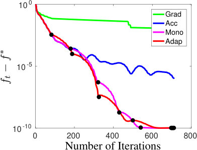 Figure 1
Peer Reviews
No public reviews on file for this paper yet. If you reviewed it on a platform where reviews are public (OpenReview, ICLR, NeurIPS, ICML), you can paste yours below so the community can read it here.
Videos
No videos yet. Explain this paper in a talk, walkthrough, or lecture? Add one.
Sharpness, Restart and Acceleration
Vincent Roulet
Department of Statistics,University of Washington, Seattle, USA.
and
Alexandre d’Aspremont
CNRS & D.I., UMR 8548,École Normale Supérieure, Paris, France.
Abstract.
The Łojasiewicz inequality shows that sharpness bounds on the minimum of convex optimization problems hold almost generically. Sharpness directly controls the performance of restart schemes, as observed by Nemirovskii and Nesterov [1985]. The constants quantifying these sharpness bounds are of course unobservable, but we show that optimal restart strategies are robust, in the sense that, in some important cases, finding the best restart scheme only requires a log scale grid search. Overall then, restart schemes generically accelerate accelerated first-order methods.
Introduction
We study111A subset of these results appeared at the NIPS 2017 conference under the same title. convex optimization problems of the form
[TABLE]
where is a convex function defined on . The complexity of these problems using first order methods is usually controlled by smoothness assumptions on such as Lipschitz continuity of its gradient. Additional assumptions such as strong or uniform convexity provide respectively linear and faster polynomial rates of convergence [Nesterov, 2013b, Juditski and Nesterov, 2014]. However, these assumptions are often too restrictive to be applicable. Here, we make a much more generic assumption that describes the growth of the function around its minimizers using constants and such that
[TABLE]
where is the minimum of , is a given set and is the Euclidean distance from to the set of minimizers of . This defines a lower bound on the function around its minimizers and quantifies the sharpness of the minimum. We exploit this property using restart schemes on classical convex optimization algorithms.
The sharpness assumption (Loja) is also known as a Hölderian error bound on the distance to the set of minimizers. Hoffman [1952] first introduced error bounds to study systems of linear inequalities. Natural extensions were then developed for convex optimization by Robinson [1975], Mangasarian [1985], Auslender and Crouzeix [1988], notably through the concept of sharp minimum [Burke and Ferris, 1993, Burke and Deng, 2002]. But the most striking result in this vein is due to Łojasiewicz [1963, 1993] who proved that inequality (Loja) holds generically for real analytic and subanalytic functions. This result has then been extended to non-smooth subanalytic convex functions by Bolte et al. [2007]. Overall then, condition (Loja) essentially measures the sharpness of minimizers, and holds generically. On the other hand, this inequality is purely implicit as or are neither observed nor known a priori, and deriving adaptive schemes is thus crucial to ensure practical relevance.
Łojasiewicz inequalities either in the form of (Loja) or as gradient dominated properties [Polyak, 1963] led to new convergence results for composite problems and for alternating or splitting methods [Attouch et al., 2010, Bolte et al., 2014, Frankel et al., 2015, Karimi et al., 2016]. Here we use this inequality to produce accelerated rates for restart schemes.
Restart schemes have already been studied for strongly or uniformly convex functions in e.g. [Nemirovskii and Nesterov, 1985, Nesterov, 2013a, Juditski and Nesterov, 2014, Lin and Xiao, 2014]. In particular, Nemirovskii and Nesterov [1985] link a “strict minimum” condition akin to (Loja) with faster convergence rates using restart schemes which form the basis of our results, but they do not study the cost of adaptation and do not tackle the non-smooth case. In a similar spirit, weaker versions of this strict minimum condition were used more recently to study the performance of restart schemes in [Renegar, 2014, Freund and Lu, 2018, Roulet et al., 2019].
The fundamental question regarding restart schemes is to define when to restart. Several heuristics have been presented that used some criterion on the iterates to restart the accelerated algorithm and speed up convergence [O’Donoghue and Candes, 2015, Su et al., 2014, Giselsson and Boyd, 2014]. However, they did not theoretically establish improved complexity bounds. The robustness of restart schemes was also studied by Fercoq and Qu [2016] for quadratic error bounds, i.e. (Loja) with , satisfied by the LASSO problem for example. Fercoq and Qu [2019] recently extended this work to produce adaptive restarts with theoretical guarantees of optimal performance, again for quadratic error bounds. In the same vein, Liu and Yang [2017] presented adaptive accelerated methods given Hölderian error bounds, but their results are not adaptive to the exponent of the error bound. The references above focus on smooth problems, but error bounds appear also for non-smooth ones, with Gilpin et al. [2012] proving for example linear convergence of restart schemes in bilinear matrix games where the minimum is sharp, i.e. (Loja) with . Recently Renegar and Grimmer [2018] presented simple generic schemes inspired by an early draft of this work, and provide adaptive schemes in all regimes (not only the smooth case).
Our contribution here is to derive optimal scheduled restart schemes for general convex optimization problems on smooth, non-smooth or Hölder smooth functions satisfying a sharpness assumption. We then show that for smooth functions these schemes can be made adaptive with nearly optimal complexity (up to a squared log term) for a wide array of sharpness assumptions. We also analyze restart schemes based on a sufficient decrease of the primal gap, when the optimal value of the problem is known. In that case, restart schemes are shown to be optimal without requiring a log scale grid search on the parameters. Our proofs only rely on having access to the convergence bound of an accelerated method, therefore our results are directly extended to the non-Euclidean case with composite objective and to non-smooth functions that can be smoothed.
1. Regularity Assumptions
1.1. Smoothness
Convex optimization problems (P) are generally divided in two classes: smooth problems, for which has Lipschitz continuous gradients, and non-smooth problems for which is not differentiable. Following Nesterov [2015], we use a unified framework that extends the definition of Hölder smooth functions.
Definition 1.1**.**
A function is -smooth for given if there exists a constant such that
[TABLE]
and any subgradients of at respectively. We write the set of -smooth functions with parameter .
For , we retrieve the classical definition of smoothness [Nesterov, 2013b]. For we get a classical assumption made in non-smooth convex optimization, i.e. that sub-gradients of the function are bounded. For we get the definition of Hölder smooth functions. We generalize our results for functions smooth with respect to a non-Euclidean norm in Section 5.
1.2. Sharpness, Error Bounds
We study convex optimization problems whose objective satisfies a growth condition as defined below.
Definition 1.2**.**
A function satisfies a Łojasiewicz growth condition on a set if there exist constants , , such that
[TABLE]
where is the minimum of , is the Euclidean distance from to the set of minimizers of . We write the set of functions satisfying a Łojasiewicz growth condition on a set with parameters , .
Condition (Loja) holds almost generically, and is notably satisfied by analytic and subanalytic functions (see [Bolte et al., 2017] for more details). However, the proof (see e.g. Bierstone and Milman [1988, Theorem 6.4]) uses topological arguments that are far from constructive. Hence, outside of some particular cases (e.g. strong convexity), we cannot assume that the constants in (Loja) are known, even approximately.
Error bounds are directly related to a Łojasiewicz inequality bounding the magnitude of the gradient [Bolte et al., 2017]. These properties underlie many recent results in optimization [Attouch et al., 2010, Frankel et al., 2015, Bolte et al., 2014]. Here, the sharpness condition in (Loja) allows us to accelerate convex optimization algorithms using restart schemes.
Our analysis relies on the condition that (Loja) is satisfied for any output of the algorithms we restart. By enforcing monotonicity of the objective values produced by those algorithms, this reduces to assume that (Loja) is satisfied on sublevel sets of the objective.
1.3. Sharpness and Smoothness
Given a convex function , by using its Taylor expansion and the smoothness property, we get for and . Setting to be the projection of onto , this yields the following upper bound on suboptimality
[TABLE]
Now, assume moreover that for a given set such that . Combining (1) and (Loja) leads to
[TABLE]
for every . This means that necessarily by taking close enough to . Moreover if , the set must satisfy .
For the following, we define
[TABLE]
a generalized condition number for the function and a condition number based on the ratio of powers in inequalities (Hölder) and (Loja), respectively. Note that if , matches the classical condition number of the function.
2. Scheduled Restarts for Smooth Convex Problems
In this section, we seek to solve (P) assuming that the function is smooth, i.e. satisfies (Hölder) with and . Without further assumptions on , an optimal algorithm to solve the smooth convex optimization problem (P) is Nesterov’s accelerated gradient method [Nesterov, 1983]. Given an initial point , this algorithm outputs, after iterations, a point
[TABLE]
where is a universal constant (whose value will be allowed to vary in what follows, with here). The accelerated algorithm can be enforced to output solutions whose objective decays monotonically as detailed in Appendix A. Consequently, if satisfies a Łojasiewicz growth condition on the initial sub-level set , then it is satisfied for any point output by the algorithm.
Note that the arguments that we develop below are not specific to the algorithm of Nesterov [1983] and would apply to any method satisfying the complexity bound (3) as shown for example in Section 5 that generalizes the results to the non-Euclidean setting. We now describe a restart scheme exploiting the extra regularity (Loja) to improve the computational complexity of solving problem (P) using accelerated methods.
2.1. Scheduled restarts
Here, we schedule the number of iterations made by the accelerated gradient algorithm between restarts, with being the number of (inner) iterations at the algorithm run (outer iteration). Our scheme is described in Algorithm 1 below.
The analysis of this scheme and the following ones rely on two steps. We first choose schedules that ensure linear convergence of the objective values w.r.t. at a given rate. We then adjust this linear rate to minimize complexity, i.e. the total number of inner iterations. We begin with a technical lemma which assumes linear convergence holds, and connects the growth of , the precision reached and the total number of inner iterations .
Lemma 2.1**.**
Let be a sequence whose iterate is generated from the previous one by an algorithm that runs iterations and write the total number of iterations to output a point . Suppose setting , for some and ensures that the outer iterations satisfy
[TABLE]
for all where and . Then, precision at the output is given by,
[TABLE]
and
[TABLE]
Proof.
When , , and inserting this in (4) at the last point yields the desired result. On the other hand, when , we have , which gives Inserting this in (4) at the last point, we get
[TABLE]
where we used . This yields the second part of the result.
The last approximation in the case simplifies the analysis that follows, without significantly affecting the bounds. We also show in Appendix B that using integer values does not significantly affect the bounds above.
We now analyze restart schedules that ensure linear convergence. Our choice of will heavily depend on the ratio between and (with for smooth functions here), measured by defined in (2). Below, we show that if , a constant schedule is sufficient to ensure linear convergence. When , we need a geometrically increasing number of iterations for each cycle.
Proposition 2.2**.**
Let be a convex function and . Denote and assume that . Run Algorithm 1 from with iteration schedule , for , where
[TABLE]
with and defined in (2) and here. The precision reached at the last point is given by,
[TABLE]
while,
[TABLE]
where is the total number of iterations.
Proof.
Our strategy is to choose such that the objective is linearly decreasing, i.e.
[TABLE]
for some depending on the choice of . This directly holds for and any . Combining (Loja) with the complexity bound in (3), we get
[TABLE]
where using that . Assuming recursively that (8) is satisfied at iteration for a given , we have
[TABLE]
and to ensure (8) at iteration , we impose
[TABLE]
Rearranging terms in this last inequality, using defined in (2), we get
[TABLE]
For a given , we can set where
[TABLE]
and Lemma 2.1 then yields,
[TABLE]
when , while
[TABLE]
when . These bounds are minimal for , which yields the desired result.
When , bound (6) matches the classical complexity bound for smooth strongly convex functions [Nesterov, 2013b]. When on the other hand, bound (7) highlights a faster convergence rate than accelerated gradient methods. The sharper the function (i.e. the closer is to ), the faster the convergence. This matches the lower bounds for optimizing smooth and sharp functions functions up to constant factors [Nemirovskii and Nesterov, 1985, Eq. 1.21]. Also, setting yields continuous bounds on precision, i.e. when , bound (7) converges to bound (6), which also shows that for near zero, constant restart schemes are almost optimal.
Note that for , the bounds (6), (7) are not informative. Precisely, the lower bounds for this problem as presented in [Nemirovskii and Nesterov, 1985, Eq. 1.21] are not informative for small . In that case, the optimal rate is given by the accelerated scheme and consequently by Algorithm 1 before the first restart.
2.2. Adaptive scheduled restart
The previous restart schedules depend on the sharpness parameters in (Loja). In general of course, these values are neither observed nor known a priori. Making the restart scheme adaptive is thus crucial to its practical performance. Fortunately, we show below that a simple logarithmic grid search on these parameters is enough to guarantee nearly optimal performance.
We begin with the following Proposition that stems from the proof of Proposition 2.2.
Proposition 2.3**.**
Let be a convex function and . Denote and assume that . Run Algorithm 1 from with general schedules of the form
[TABLE]
If and , then
[TABLE]
while, if and , then
[TABLE]
where
[TABLE]
and is the total number of iterations.
Proof.
Given general schedules of the form
[TABLE]
the best value of satisfying condition (10) for any in Proposition 2.2 is given by
[TABLE]
As in Proposition 2.2, plugging these values into the bounds of Lemma 2.1 yields the desired result.
We run several schemes with a fixed number of inner iterations to perform a log-scale grid search on and . We define these schemes as follows.
[TABLE]
where and . We stop each of these schemes when the total number of its inner iterations has exceeded , i.e. at the smallest such that . The size of the grid search in is naturally bounded as we cannot restart the algorithm after more than total inner iterations, so . We also show that when is smaller than , a constant schedule where performs as well as the optimal geometrically increasing schedule where . This crucially means we can also choose , hence limiting the cost of the grid search.
The following proposition details the convergence of this grid-search, using the same notations as in Proposition 2.2. As observed at the end of Section 2.1, the optimal bounds (6), (7) are only informative after a sufficient number of iterations, which is why we analyze the adaptive scheme only for a number of iterations . To get optimal bounds in all regimes, it suffices to run an additional non-restarted algorithm that will also capture the best rate in the case .
Proposition 2.4**.**
Let be a convex function and . Denote , assume that and denote by a given number of iterations.
Run schemes defined in (15) to solve (P) for and , stopping each time after total inner algorithm iterations, i.e. for such that .
If , there exists such that the scheme achieves a precision given by
[TABLE]
If , there exist and such that the scheme achieves a precision given by
[TABLE]
Overall, running the logarithmic grid search has a complexity times higher than running iterations using the optimal (oracle) scheme.
Proof.
Denote the number of restarts of a scheme , we have for , and for , . Denote the number of iterations of a scheme . We necessarily have for our choice of and . Hence the cost of running all methods is of the order of .
If and , then . Therefore has been run and bound (12) shows then that the last iterate satisfies
[TABLE]
Using that ,
[TABLE]
If and , then and . Therefore scheme has been run. As , where is defined in (14), bound (13) shows that the last iterate of scheme satisfies
[TABLE]
Finally, by definition of and , and , so
[TABLE]
where we concluded by expanding and using that .
If and , then , so scheme has been run. As in (9), its iterates satisfy, with ,
[TABLE]
Now and , therefore last iterate satisfies
[TABLE]
As , since is decreasing with and , we have
[TABLE]
having used the facts that if , and when . As , we finally get
[TABLE]
using the fact that .
In the strongly convex case, this adaptive bound is similar to the one of [Nesterov, 2013a] to optimize smooth strongly convex functions in the sense that we lose approximately a log factor of the condition number of the function. However our assumptions are weaker and our bound also handles all sharpness regimes, i.e. any exponent , not just the strongly convex case. Finally the step size chosen for the grid search was set to 2. The proof can be adapted for a generic step size , the size of the grid may be reduced but corresponding bounds will suffer an approximation loss compared to the best schedule.
Note that the scheduled restart schemes we present here adapt to a global sharpness hypothesis on the sublevel set defined by the initial point and are not locally adaptive to potentially better constant on smaller sublevel sets. On the other hand, restart schemes based on a primal gap, presented in Section 4, do adapt to the local value of , although these schemes require having access to the primal gap.
2.3. Comparison to gradient descent
We end this section by analyzing the behavior of gradient descent in light of the sharpness assumption in order to compare the advantage of restarted accelerated method to plain gradient descent. While the bounds we obtain using the basic gradient method are suboptimal compared to the ones above, the gradient algorithm having no memory will automatically adapt to the best “restart” schedule. Given only the smoothness hypothesis, the gradient descent algorithm, presented in e.g. [Nesterov, 2015], starts from a point and outputs iterates
[TABLE]
While accelerated methods use the last two iterates to compute the next one, simple gradient descent algorithms use only the last iterate, so the algorithm can be seen as (implicitly) restarting at each iteration. Formally we use that its convergence can be bounded as, for ,
[TABLE]
and we analyze it in light of the restart interpretation using the sharpness property.
Proposition 2.5**.**
Let be a convex function and . Denote and assume that . Denote by the iterate sequence generated by the gradient descent algorithm started at to solve (P) and define
[TABLE]
with and defined in (2) and here. The precision reached after iterations is given by,
[TABLE]
while,
[TABLE]
Proof.
For a given , we construct a subsequence of such that
[TABLE]
Define . Assume that (17) is true at iteration , then combining complexity bound (16) and (Loja), for any ,
[TABLE]
where , using that . Taking and ensures that (17) holds at iteration . Using Lemma 2.1, we obtain at iteration ,
[TABLE]
and
[TABLE]
These bounds are minimal for and the results follow.
We observe that restarting accelerated gradient methods reduces complexity from to compared to simple gradient descent. More general results on the convergence of (sub)gradient descent algorithms under a Łojasiewicz inequality assumption were developed by Bolte et al. [2017].
3. Universal Scheduled Restarts for Convex Problems
In this section, we generalize previous results to -smooth functions as defined in Definition 1.1 to tackle both smooth and non-smooth convex optimization problems. Without further assumptions on , the optimal rate of convergence for this class of functions is bounded as , where is the total number of iterations and
[TABLE]
which gives for smooth functions and for non-smooth functions. The universal fast gradient method [Nesterov, 2015] achieves this rate by requiring only a target accuracy and a starting point . It outputs after iterations a point
[TABLE]
where is a constant (). A simplified implementation of the universal fast gradient method that enforces monotonicity in objective values of the outputs of the algorithm is presented in Appendix A.
We assume again that satisfies a Łojasiewicz growth condition on its initial sublevel set. The key difference with the smooth case described in the previous section is that here we schedule both the target accuracy used by the algorithm and the number of iterations made at the run of the algorithm. Our scheme is described in Algorithm 2.
Our strategy is to choose a sequence that ensures
[TABLE]
for the geometrically decreasing sequence . The overall complexity of our method will then depend on the growth of as described in Lemma 2.1.
Proposition 3.1**.**
Let be a convex function and . Denote and assume that . Run Algorithm 2 from for a given with
[TABLE]
where is defined in (18), and are defined in (2) and here. The precision reached at the last point is given by,
[TABLE]
while,
[TABLE]
where is total number of iterations.
Proof.
Our goal is to ensure that the target accuracy is reached at each restart, i.e.
[TABLE]
By assumption, (20) holds for . Assume that (20) is true at iteration , combining (Loja) with the complexity bound in (19), then
[TABLE]
where using that . By definition , so to ensure (20) at iteration this imposes
[TABLE]
Rearranging terms in last inequality, using defined in (2),
[TABLE]
Choosing , where
[TABLE]
and using Lemma 2.1 then yields,
[TABLE]
when , while,
[TABLE]
when . These bounds are minimal for and the results follow.
This bound matches the lower bounds for optimizing smooth and sharp functions up to constant factors [Nemirovskii and Nesterov, 1985, Eq. 1.21]. Notice that, compared to Nemirovskii and Nesterov [1985], we can tackle non-smooth convex optimization by using the universal fast gradient algorithm of Nesterov [2015]. The rate of convergence in Proposition 3.1 is controlled by the ratio between and . If these are unknown, a log-scale grid search will not be able to reach the optimal rate, even if is known since we will miss the optimal rate by a constant factor, see Appendix C. If both are known, in the case of non-smooth strongly convex functions for example, a grid-search on recovers a nearly optimal bound. Finally note that our bound is provided with respect to the number of iterations of the accelerated algorithms, the corresponding bounds in terms of numbers of calls to the oracles can be found by analyzing the line-search cost of the fast universal gradient method.
4. Restart With Known Primal Gap
Here, we assume that we know the optimum of (P). This is the case for example in zero-sum matrix game problems or over-parametrized least-squares without regularization. We assume again that satisfies the generic smoothness assumption (Hölder) and the Łojasiewicz growth condition (Loja) on its initial sublevel set. We use again the universal gradient method . Here however, we can stop the algorithm when it reaches the target accuracy as we know the optimum , i.e. we stop after inner iterations such that satisfies , and write the output of this method.
Here we simply restart this method and decrease the target accuracy by a constant factor after each restart. Our scheme is described in Algorithm 3. The following proposition describes its convergence.
Proposition 4.1**.**
Let be a convex function and . Denote and assume that . Run Algorithm 3 from with parameter . The precision reached at the last point is given by,
[TABLE]
while,
[TABLE]
where is the total number of iterations, is defined in (18), and are defined in (2) and here. Those bounds are suboptimal to the best scheduled restarts by a factor at most .
Proof.
Given , the linear convergence of our scheme is ensured by our choice of target accuracies . It remains to compute the number of iterations needed by the algorithm before the restart. Following the proof of Proposition 3.1, for we know that the target accuracy is necessarily reached after
[TABLE]
iterations, such that . So Algorithm 3 achieves linear convergence while needing less inner iterates than the scheduled restart presented in Proposition 3.1, its convergence is therefore at least as good. For a given bounds (22) and (23) follow with . The dependency in of the restart scheme in bounds (22) and (23) is a factor
[TABLE]
of the number of iterations, whose maximum value is reached for . Taking , then leads to a bound suboptimal by a constant factor of at most for , so running this scheme with makes it parameter-free while producing nearly optimal complexity.
When is known, the above restart scheme is adaptive, contrary to the general non-smooth case in Proposition 3.1. It can even adapt to the local values of or as we use a criterion instead of a preset schedule. Here, stopping using implicitly yields optimal choices of and . Note that this approach generalizes to algorithms for which a bound on the primal gap is available as in the Frank-Wolfe algorithm, see [Kerdreux et al., 2019].
5. Extensions
Previous analyses of restart schemes only require bounds of the form (3) or (19). Our results extend then readily to non-Euclidean composite settings or structured objectives as presented below.
5.1. Composite Problems & Bregman Divergences
We extend previous schemes to more general convex optimization problems of the form
[TABLE]
where is a simple convex function (the meaning of simple will be clarified later), is a convex -smooth function with respect to a given norm (potentially non-Euclidean) as defined below, and is defined on an open-set containing , i.e. .
Definition 5.1**.**
A function is -smooth for a given with respect to a norm if there exists a constant such that
[TABLE]
and any subgradients of at respectively, with being the dual norm of . We denote by the set of -smooth functions with respect to a norm with parameter .
To exploit the smoothness of with respect to a generic norm, we assume that we have access to a potential function with , strongly convex with respect to the norm with convexity parameter equal to one, which means
[TABLE]
We define the Bregman divergence associated to as, for given ,
[TABLE]
For , we get and recover the Euclidean setting. Given the problem geometry, appropriate choices of potential functions and associated Bregman divergences can lead to significant performance gains in high dimensional settings. We now formally state the assumption that is simple. Given and we assume that
[TABLE]
can be solved either in a closed form or by some fast computational procedure.
This setting includes some constrained optimization problems, where is the indicator function of a closed convex set, on which we can easily project the points. It also includes sparse optimization problems, such as the LASSO, where , with , , , with and . To apply our analysis of restart schemes we need two things: an accelerated algorithm and an appropriate notion of sharpness. In the spirit of [Bauschke et al., 2016, Lu et al., 2018], we thus introduce the notion of relative sharpness.
Definition 5.2**.**
A function satisfies a relative Łojasiewicz growth condition with respect to a strictly convex function on a set if there exist , such that
[TABLE]
where and is the Bregman divergence associated to . We denote by the set of functions satisfying a relative Łojasiewicz growth condition w.r.t to on a set with parameters .
If we recover the definition of the Łojasiewicz growth in the Euclidean setting (with slightly modified constants). This assumption is as generic as our first one in (Loja) as it is satisfied if and are subanalytic [Bierstone and Milman, 1988, Th. 6.4].
The algorithms are essentially the same as before, except that the distance to the set of minimizers is replaced by the Bregman divergence to the set of minimizers. We keep the same notations for the algorithms as the implementations are the same as presented in Section A. Formally, if is smooth with respect to a norm , the accelerated algorithm outputs after iterations a point
[TABLE]
where here. The next Corollary generalizes Proposition 2.2.
Corollary 5.3**.**
Let be a composite convex function, and . Assume that for a given norm , that for strongly convex with respect to and that is simple such that problems (25) can be computed efficiently. Run Algorithm 1 from with iteration schedule , for , where
[TABLE]
with and defined in (2) and . The precision reached at the last point is given by,
[TABLE]
while,
[TABLE]
where is the total number of iterations.
Proof.
The proof of Proposition 2.2 only relies on the bound in (9) that combines the growth condition (Loja) with the complexity bound in (3). For the case with composite problems and Bregman divergences we combine (26) with the bound (27), which ensures for the th iterate of the restart scheme, with here . The rest of the proof follows as in Proposition 2.2.
For general convex functions, given a target accuracy and an initial point , the universal fast gradient method outputs after iterations a point
[TABLE]
where here. The following Corollary generalizes then Proposition 3.1.
Corollary 5.4**.**
Let be a composite convex function, and . Assume that for a given norm , that for strongly convex with respect to and that is simple such that problems (25) can be computed efficiently. Run Algorithm 2 from for given ,
[TABLE]
where is defined in (18), and are defined in (2) and . The precision reached at the last point is given by,
[TABLE]
while,
[TABLE]
where is total number of iterations.
Proof.
The proof of Proposition 3.1 only relies on the bound in (21) that combines the growth condition (Loja) with the complexity bound in (19). For the case with composite problems and Bregman divergences we combine (26) with the bound (28), which ensures for the th iterate of the restart scheme, with here . The rest of the proof follows as in Proposition 3.1.
The results regarding adaptive schemes and those for which is known, i.e. Propositions 2.4 and 4.1 respectively, generalize similarly under the relative growth assumption. Those results apply then to generic regularized prediction problems where is an norm and is a data-fitting term. Indeed error bounds were proven to hold for those problems by Zhou et al. [2015]. Those error bounds are then equivalent to quadratic growth conditions, i.e. (Loja) with [Drusvyatskiy and Lewis, 2018]. Previous works demonstrate then linear convergence of proximal gradient descent [Bolte et al., 2017]. Here the restart schemes allow to get accelerated rates similar as for smooth strongly convex problems. Note that adaptive schemes were also developed by [Fercoq and Qu, 2019] in that case.
5.2. Smoothing non-smooth problems
Our approach extends also to problems that can be smoothed, i.e. problems of the form
[TABLE]
where , is a simple convex function and is a non-smooth convex function whose inf-convolution with some smooth convex function can be computed analytically, i.e. one has access for any to
[TABLE]
where for a function we denote by its convex conjugate. Those problems were notably considered by Nesterov [2005], who proved that, though they a priori suffer from their non-smoothness, they can still be solved in calls to an oracle by using their structure. Formally, we have access to an algorithm that, given an initial point and a target accuracy , outputs after iterations a point
[TABLE]
where is some potential function and is a smoothing constant, see Appendix A for more details. The scheduled restarts of this algorithm will follow the same strategy as for the fast universal gradient method as presented in the following proposition.
Proposition 5.5**.**
Let be a non-smooth objective that can be smoothed using (30), and . Assume that we have access to a smoothing method ensuring (31) for a given strongly convex function and that . Given , restart the method such that for ,
[TABLE]
where and are defined as in (2) with and in place of .
The precision reached at a point after restarts is given by,
[TABLE]
while,
[TABLE]
where is total number of iterations.
Proof.
The smoothing method has a bound of the same form as the universal fast gradient method, i.e. we have
[TABLE]
with here , and . The optimal restart schedule and corresponding rates follow then from Proposition 3.1 by replacing and .
As for the universal fast gradient method, a grid-search will not get optimal rates if and so is unknown. However if it is known, a grid-search will ensure optimal rates up to a constant factor. It is illustrated for sparse recovery problems by Roulet et al. [2019].
If is known, Proposition 4.1 is modified into the following proposition. Note that the resulting restart scheme is the one presented by Gilpin et al. [2012] for zero-sum matrix games.
Proposition 5.6**.**
Let be a non-smooth objective that can be smoothed using (30), and . Assume that is known, that we have access to a smoothing method ensuring (31) for a given strongly convex function and that . Denoting , consider the restart scheme defined by
[TABLE]
The precision reached at a point after restarts is given by,
[TABLE]
while,
[TABLE]
where is total number of iterations and and are defined as in (2) with and in place of .
Proof.
As in Proposition 4.1, the proposed scheme with a termination criterion on the gap cannot do worse than the optimal scheduled restart. The rate is then given by Proposition 5.5.
6. Numerical Results
We illustrate our results by testing our adaptive restart schemes, the adaptive scheme Adap of Section 2.2, and the scheme with stopping criterion on the primal gap Crit in Section 4, on several problems to compare them against simple gradient descent (Grad), accelerated gradient methods (Acc), and the restart heuristic enforcing monotonicity (Mono) proposed by [O’Donoghue and Candes, 2015]. For Adap we plot the convergence of the best method found by grid search to compare with the restart heuristic. This implicitly assumes that the grid search is run in parallel with enough servers. For Crit we use the optimal found by another solver. This gives an overview of its performance when such information is available. All restart schemes were performed using the accelerated gradient with backtracking line search detailed in Appendix A, with large dots representing restart iterations.
In Figure 1, we solve classification problems with various losses on the UCI Sonar data set [Asuncion and Newman, 2007]. For the least square loss on sonar data set, we observe much faster convergence of the restart schemes compared to the accelerated method. These results were already observed by O’Donoghue and Candes [2015]. For the logistic loss, we observe that restart does not provide much improvement for a budget of 1000 iterations. For the hinge loss, we regularized by a squared norm and optimize the dual, which means solving a quadratic problem with box constraints. We observe here that the scheduled restart scheme converges much faster, while restart heuristics may be activated too late. We observe similar results for the LASSO problem. This highlights the benefits of a sharpness assumption for these last two problems. In general Crit ensures the theoretical accelerated rate but Adap exhibits more consistent behavior. Again, precisely quantifying sharpness from data/problem structure is a key open problem.
To account for the grid search effort, in Figure 2, we multiplied the number of iterations made by the Adap method by the size of the grid. This is for the LASSO problem on Sonar data set with a grid step size of . This shows that the benefits of the restart schemes make the grid search effort acceptable both on paper and in practice. More clever grid search strategies for scheduled restarts run in parallel would even reduce this effort.
Acknowledgments
AA is at CNRS, attached to the Département d’Informatique at École Normale Supérieure in Paris, INRIA-Sierra team, PSL Research University. VR is in the Statistics Department of the University of Washington, working for the Algorithmic Foundations of Data Science Institute. The authors would like to acknowledge support from the fonds AXA pour la recherche, a gift from Société Générale Cross Asset Quantitative Research, an AMX fellowship and a Google focused award.
Appendix A Algorithms & Complexity Bounds
We present here the algorithms that we restart. In particular we present a simplified version of the universal fast-gradient method of Nesterov [2015] and shows how we can enforce monotonicity of the objective values, while keeping the optimal rate. The classical accelerated algorithm for smooth convex function is then derived as a special case of the universal method.
In both cases the smoothness constant do not need to be known in advance. A line-search is provided whose complexity can be bounded as done in [Nesterov, 2015]. In practice when restarting the algorithm we use the last smoothness constant provided by the algorithm.
A.1. Problem formulation
We focus on composite optimization problems of the form
[TABLE]
where are proper lower semi-continuous convex functions on and is defined on an open-set containing , i.e. . We denote a given norm on and the dual norm of .
We assume that is -smooth with respect to for a given , i.e. that there exists such that
[TABLE]
for all and any . We assume that we have access to a function , differentiable on its domain , strongly convex with respect to the norm with convexity parameter equal to one, i.e.
[TABLE]
We define the Bregman divergence associated to as, for given ,
[TABLE]
Finally we assume that, for any and we can solve
[TABLE]
either in a closed form or by some cheap computational procedure. In the following, we denote for any ,
[TABLE]
where is any sub-gradient of at . This partial linearization of the objective is convex and satisfies by convexity of ,
[TABLE]
A.2. Universal fast gradient method
Our simplified version of the Universal Fast Gradient method is presented in Algorithm 4. Proposition A.1 shows the convergence of Algorithm 4. Proposition A.2 ensures that the line-searches terminate. The total number of oracle calls can be bounded as done by Nesterov [2015], using a termination criterion, we only give the complexity in terms of iterations of the algorithm. Monotonicity is enforced by simply taking the best of the new and old iterate at each iteration.
Proposition A.1**.**
Consider problem (32) where satisfies (33) with parameters . Algorithm 4, started at an initial point for a target accuracy and an initial estimate , outputs after iterations a point such that
[TABLE]
where with .
Proof.
Monotonicity of the objective values is ensured by (43). We fix in the following . Consider the th iteration of Algorithm 4 for . We have
[TABLE]
where in we used that , the convexity of and . Subtracting on both sides and dividing by , we get
[TABLE]
If , we have, using the initialization , ,
[TABLE]
Otherwise we have using the definition of in (41),
[TABLE]
Using inequality (38) recursively from to and inequality (37) for we get
[TABLE]
Finally a bound on can be found by combining Proposition A.2 and Proposition A.1 such that and we get, denoting ,
[TABLE]
Taking concludes the proof.
Proposition A.2**.**
Consider problem (32) where satisfies (33) with parameters . The line-searches of Algorithm 4 terminate with
[TABLE]
Proof.
Lemma A.4 ensures that the line-search for stops for Therefore we have . For , during the line-search procedure, the parameter reads, denoting , . Using again Lemma A.4, the stopping criterion (42) is then ensured if there exists such that
[TABLE]
Denote for . We have . Therefore there exists satisfying (40). Moreover the line-search terminates with as otherwise, and the line-search would have stopped before.
A.3. Accelerated algorithm
The accelerated algorithm is obtained as a special case of the universal fast gradient algorithm for and a choice of , i.e., . Its rate follows from the one given by the universal fast gradient method as recalled below.
Corollary A.3**.**
Consider problem (32) where satisfies (33) with parameters . Algorithm 4 with , started at an initial point with an initial estimate , outputs after iterations a point such that
[TABLE]
where with .
A.4. Lemmas for proving convergence
Lemma A.4** ([Nesterov, 2015, Lemma 2]).**
Let satisfying (33). Then for any and or a fortiori any we have, for any and ,
[TABLE]
Lemma A.5** ([Tseng, 2008, Property 1]).**
For any proper l.s.c. convex function , and any , denote Then for any ,
[TABLE]
Lemma A.6**.**
Consider two sequences initialized by and satisfying
[TABLE]
for some , with . Then for any ,
[TABLE]
Proof.
The first property of (47) is true for since . The definition of for reads then which shows the first property (47) by induction.
For , denote and , such that . We have from (46), . Therefore which gives Denote and . Since and , we have for any ,
[TABLE]
Therefore we conclude that
A.5. Smoothing non-smooth problems
We present here the smoothing algorithm used in Section 5. We recall the problem
[TABLE]
where , is a simple convex function and is a non-smooth convex function whose inf-convolution with some smooth convex function can be computed analytically, i.e. one has access for any to
[TABLE]
where for a function we denote by its convex conjugate, see [Beck and Teboulle, 2012] for a detailed exposition. For 1-strongly convex w.r.t. a given norm (i.e. 1-smooth w.rt. ), the function is smooth w.r.t. the norm . Moreover it approximates as (see e.g. [Pillutla et al., 2018, Proposition 41])
[TABLE]
The smoothed objective is a composite objective as in (32), i.e.,
[TABLE]
where, denoting , we have that is smooth w.r.t. a norm (see e.g. [Pillutla et al., 2018, Lemma 42]). We can then apply the accelerated algorithm on (50) with a potential function strongly convex w.r.t. the norm , assuming that is simple such that we have access to oracles of the form (25). Precisely, given an initial point and a target accuracy , by applying the accelerated algorithm on (50) with , where , we get after iterations a point such that for ,
[TABLE]
where in we use the definition of and the convergence bound (39) of the accelerated algorithm () applied on . We denote then any point such that such that it satisfies both the rate above and belongs to the initial sub-level set. The bound presented in equation (31) is obtained by taking and defining and .
Appendix B Rounding issues
We presented convergence bounds for real sequences of iterate counts but in practice these are integer sequences. The following Lemma details the convergence of our schemes for an approximate choice .
Lemma B.1**.**
Let be a sequence whose iterate is generated from previous one by an algorithm that needs iterations and denote the total number of iterations to output a point . Suppose setting for some and ensures that objective values converge linearly, i.e.
[TABLE]
for all with and . Then precision at the output is given by,
[TABLE]
and, denoting ,
[TABLE]
Proof.
At the point generated, . If , define such that . Then , injecting it in (51) at the point,
[TABLE]
Now, if , define , such that . On one hand such that On the other hand,
[TABLE]
such that Injecting it in (51) at the point the result follows.
Appendix C Grid-search for universal restart schemes
We briefly explain why a grid-search on the parameters for the general case does not provide near-optimal bounds. Consider general restart schemes as presented in Algorithm 2 for a function with the initial sublevel set of at a given . Assume that the decreasing factor is and the schedules have the form such that
[TABLE]
which is and . Consider the case . Then following the proof of Proposition 3.1, we get that and applying Lemma 2.1 we obtain a convergence rate
[TABLE]
where is the total number of iterations. For this rate to be optimal or nearly optimal we need . Any grid search on this ratio will then suffer from a constant factor such that we won’t get a rate of the form except if we know and which gives us .
The reference list from the paper itself. Each links out to its DOI / PubMed record.
- 1[1]
- 2Arjevani and Shamir [2016] Arjevani, Y. and Shamir, O. [2016], On the iteration complexity of oblivious first-order optimization algorithms, in ‘Proceedings of the 33rd International Conference on Machine Learning’, Vol. 48, pp. 908–916.
- 3Asuncion and Newman [2007] Asuncion, A. and Newman, D. [2007], ‘UCI machine learning repository’.
- 4Attouch et al. [2010] Attouch, H., Bolte, J., Redont, P. and Soubeyran, A. [2010], ‘Proximal alternating minimization and projection methods for nonconvex problems: An approach based on the Kurdyka-Łojasiewicz inequality’, Mathematics of Operations Research 35 (2), 438–457.
- 5Auslender and Crouzeix [1988] Auslender, A. and Crouzeix, J.-P. [1988], ‘Global regularity theorems’, Mathematics of Operations Research 13 (2), 243–253.
- 6Bauschke et al. [2016] Bauschke, H. H., Bolte, J. and Teboulle, M. [2016], ‘A descent lemma beyond lipschitz gradient continuity: first-order methods revisited and applications’, Mathematics of Operations Research 42 (2), 330–348.
- 7Beck and Teboulle [2012] Beck, A. and Teboulle, M. [2012], ‘Smoothing and first order methods: A unified framework’, SIAM Journal on Optimization 22 (2), 557–580.
- 8Bierstone and Milman [1988] Bierstone, E. and Milman, P. D. [1988], ‘Semianalytic and subanalytic sets’, Publications Mathématiques de l’IHÉS 67 , 5–42.